An Evaluation of the Current Sediment Basin Designs in North Carolina and Evaluating the Applicability of Designing Sedimentation Basins on North Carolina Department of Transportation Highway Construction Sites with RUSLE2.

(1)

North Carolina Department of Transportation Highway Construction Sites with RUSLE2. (Under the direction of Dr. Greg Jennings and Dr. Rich McLaughlin).

The rapid population growth and the resulting construction of buildings and roads can result in increased erosion and sediment discharge into streams, lakes, and rivers. This sediment can dramatically decrease the water quality and impair the ecosystems within and around these bodies of water. To be incompliance with the Clean Water Act, North Carolina Department of Transportation is required to develop sediment and erosion control plans for highway construction projects. Sediment basins are a typical best management practice used on these sites, and in recent years there has been an interest in evaluating the current design, tracking the dynamic changes in the landscape over the course of the project, and applying a more process based approach. One option is to use the robust computer application for estimating soil erosion, RUSLE2, in order to determine sediment yields and appropriately size sediment basins.

Based on repeated surveys of a highway construction project site, there was a progression from the natural and original contours to a catchment with a flat interior for the road bed with relatively steep slopes at the edges and showed no relationship of changing sediment yields to the average slope of the catchment.

From monitoring the sediment yields through the progression of the project, there tended to be an increase in sediment yield and total suspended solids concentration as

(2)

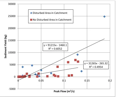
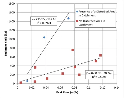
and whether the catchment area is disturbed. The performance of the basin was dictated by the intensity of the storm event, and this basin performance in terms of removing sediment and turbidity may be more accurately predicted for lower intensity storms. This analysis suggests that intensity as a sole parameter may be an important consideration in establishing criteria for a desired basin performance in terms of a reduction of turbidity. The sediment yields were well correlated to the stormwater volume reaching the basin as well as the peak flow from a storm event. Most notably was the correlation of the presence of an uncovered, disturbed area to sediment yield entering the basin which indicates that cover is crucial in preventing soil erosion.

Based on a comparison of RUSLE2 sediment yield predictions to field measured sediment yield, it is not advised to use RUSLE2 as a reliable method for estimating sediment yields with the current practices on these construction sites. The estimates given by RUSLE2 tend to be much less than actual sediment yield measured in the field due to erosion in the unprotected ditches and diversions leading to the basins. A combination of channel erosion, maintenance practices, and site management increased sediment yields to the basins beyond what RUSLE2 is capable of predicting and how the model should be used. Either the use of another model which includes channel erosion or management practices that reduce or eliminate channel erosion with relatively stable catchments is recommended.

(3)

(4)

(5)

by

Ryan Francis Brown

A thesis submitted to the Graduate Faculty of North Carolina State University

in partial fulfillment of the requirements for the degree of

Master of Science

Biological and Agricultural Engineering

Raleigh, North Carolina 2012

APPROVED BY:

_______________________________ ______________________________

Dr. Gregory D. Jennings Dr. Richard A. McLaughlin

Committee Chair

(6)

DEDICATION

(7)

BIOGRAPHY

It was a dark, cold, and blizzard filled night in the winter of 1988 when Ryan Francis Brown was born to James and Frances Brown in Charlotte, NC. Earlier in the night, North Carolina and Duke squared off in an intense hoopfest. Duke inevitably won the contest, but in hind sight was probably a good thing so that Ryan didn’t have to live through more UNC losses than was entirely necessary.

His family moved to Irmo, SC in on April Fool’s Day in 1996 where he became a member of the Bands of Irmo, with whom he performed great works of music ranging from Hot Cross Buns to Carmina Burana in some of the greatest music halls in the country including the Atlanta Symphony Hall, Carnegie Hall, and the RCA Dome in Indianapolis.

After considering a wide range of professions through his life from a rock star to an orthopedic surgeon to a financial professional, he decided engineering focused on biology and the environment thanks to the influences of his teachers and brother, Justin.

He attended Clemson University where he received a BS in biosystems engineering in 2010. During his time there he met his lovely wife, Audrey, to whom he was wed to after they had graduated.

He attempted to find a job near his soon to be wife, but due to the great recession those ideas were stunted and therefore he ended up pursuing an MS in Biological and Agricultural

(8)

ACKNOWLEDGMENTS

Audrey, for support; My family, for their belief and guidance; My teachers and advisors, for their inspiration and willingness; Society, for funding and having a genuine interest; Music,

for its transcending power.

I would also like to thank all of the people with the set up and data collection for this project; Jamie Luther, Virginia Brown, Gina Lee, Kim Whitley, Melanie McCaleb, Rich

McLaughlin, Rob Austin, and Paul Worthington.

The North Carolina DOT for funding the project and Raleigh-Durham Road Builders, specifically Mike Tuszynski, for their cooperation and aid.

(9)

TABLE OF CONTENTS

LIST OF TABLES………...viii

LIST OF FIGURES………...xxix

CHAPTER 1: LITERATURE REVIEW... 1

1.1 EROSION ON CONSTRUCTION SITES: THE EFFECTS AND REGULATIONS ... 1

1.2 PLANNING FOR AND CONTROLLING EROSION ... 2

1.3 THE EVOLUTION OF USLE ... 4

1.4 USES AND EVALUATIONS OF RUSLE2 FOR CONSTRUCTION SITE EROSION CONTROL PLANNING ... 6

1.5 GULLY EROSION ... 9

1.6 RESEARCH NEED ... 10

CHAPTER 2: SURVEYS AND CHANGES IN TOPOGRAPHY ... 12

2.1 INTRODUCTION ... 12

2.2 METHODS AND MATERIALS ... 14

2.2.1 Survey Techniques of Catchments ... 14

2.2.2 Survey Post-Processing for Application to RUSLE2 ... 15

2.2.3 Data Analysis ... 15

2.3 RESULTS AND DISCUSSION ... 16

2.4 CONCLUSIONS ... 20

CHAPTER 3: ANALYSIS OF SEDIMENT YIELDS AND BASIN PERFORMANCE WITH RELATION TO CURRENT SKIMMER BASIN SIZING METHODS ... 21

(10)

3.2.1 Sediment Basin Monitoring ... 22

3.2.2 Site and Basin Descriptions ... 26

3.3.1 Changes in Sediment Load over Time ... 38

3.3.2 Using Pearson’s Correlation Coefficient for Single Variable Relationships ... 45

3.3.3 Basin Performance by Reduction in Turbidity as Dependent Variable ... 48

3.3.4 Sediment Entering Basin at Inlet as Dependent Variable ... 53

3.4 CONCLUSION ... 61

3.4.1 Changes in Sediment Yields through Progression of Projects ... 61

3.4.2 Basin Performance by Reduction in Turbidity ... 62

3.4.3 Sediment Entering Basin ... 63

CHAPTER 4: EVALUATION OF RUSLE2 MODEL FOR PREDICTING SEDIMENT YIELDS ON A PIEDMONT NORTH CAROLINA HIGHWAY CONSTRUCTION SITE ... 65

4.1 INTRODUCTION ... 65

4.2.1 Sediment Basin Monitoring ... 68

4.2.2 Site Descriptions ... 70

4.2.3 Site Soil Analysis ... 71

4.2.4 RUSLE2 Profile Development from Processed Surveys ... 72

(11)

4.3.1 Comparing Field Sediment Yields to RUSLE2 Calculations ... 79

4.3.2 Sensitivity of Topographic Element in RUSLE2 ... 96

4.4 CONCLUSION ... 105

4.4.1 Comparing RUSLE2 estimates using topography from surveys to field results ... 105

4.4.2 Comparing RUSLE2 estimates using planning set topography to the field sediment yields ... 107

4.4.3 Comparing RUSLE2 estimates on a storm-by-storm basis to the field sediment yields ... 107

4.4.2 Sensitivity of Topography in RUSLE2 Calculations ... 108

REFERENCES ... 109

APPENDICES ... 117

APPENDIX A ... 118

APPENDIX B ... 179

APPENDIX C ... 217

APPENDIX D ... 256

(12)

LIST OF TABLES

Table 2-1. Average slope in catchment of Basin 11.4 B for respective survey. Surveys taken with total station or LiDAR as noted. ... 18 Table 2-2. Average slope in catchment of Basin 9.2 C for respective survey. All surveys taken with LiDAR. ... 18 Table 2-3. Average slope in catchment of Basin 10.3 B for respective survey. All

surveys taken with LiDAR. ... 19 Table 2-4. Average slope in catchment of Basin 5.10 B for respective survey. All

(13)

Table 3-7. Design dimension and calculations for Basin ID 5.10 B from clearing and grubbing plans. ... 33 Table 3-8. Basin efficiency in terms of reduction of turbidity, reduction of average TSS, and reduction of total sediment for each storm collected. ... 49 Table 3-9. Parameter estimates for selected variables within stepwise function with basin performance by reduction in turbidity for all storms with inflow and outflow. ... 51 Table 3-10. Parameter estimate for selected variables within the stepwise function with sediment yield as dependent variable for all storms with inflow samples collected. ... 56 Table 3-11. Parameter estimate for selected variables within the stepwise function with sediment yield as the dependent variable for all storms collected on Basin 11.4 B. ... 58 Table 3-12. Parameter estimates for selected parameters in stepwise function on Basin 9.2 C. These are given for a relative sense of impact the selected independent variable had on the sediment yield. ... 59 Table 3-13. Parameter estimates for selected parameters in stepwise function on Basin 5.10 B. These estimates are given for a relative sense of the impact the selected

(14)

Table 4-2. Parameter estimates of the slope and intercept of the regression model using data based on survey topography. Model is: DIFF = (Slope)*(RUSLE2 Estimate) + Intercept + error. ... 80 Table 4-3. Parameter estimates of the slope and intercept of the regression model using data based on survey topography without data point from Basin 5.10 B. Model is: DIFF = (Slope)*(RUSLE2 Estimate) + Intercept + error. ... 80 Table 4-4. Results of the sediment yield from the field and RUSLE2 calculations using representative slopes and average slopes from plans. Basins 11.4 B and 9.2 C included a clearing and grubbing (CG) phase and mass grading (MG) phase. Basin 10.3 B included a final grade (FG) and post paving (PP) phase. Basin 5.10 B included a

clearing and grubbing (CG) phase. ... 84 Table 4-5. Parameter estimates of the slope and intercept of the regression model using data based on planning phase topography. Model is: DIFF = (Slope)*(RUSLE2

Estimate) + Intercept + error. ... 85 Table 4-6. Parameter estimates of the slope and intercept of the regression model without using data point from Basin 5.10 B using data based on planning phase

topography. Model is: DIFF = (Slope)*(RUSLE2 Estimate) + Intercept + error. ... 85 Table 4-7. Parameter estimates of the slope of the regression model using data based the on average slope of the catchment in the planning phase. Model is: DIFF =

(15)

Table 4-8. Parameter estimates of the slope of the regression model without using data point from Basin 5.10 B using data based on the average slope of the catchment in the planning phase. Model is: DIFF = (Slope)*(RUSLE2 Estimate) + Intercept + error. .. 86 Table 4-9. Results from RUSLE2 sediment calculation using respective survey

topography for individual storms and field sediment yields. ... 87 Table 4-10. Parameter estimates of the slope and intercept in the regression model using the RUSLE2 on an individual storm basis with the respective survey for

(16)

Table 4-15. For storms collected with intensities less than 12.7 mm/hr, Parameter estimates of the slope and intercept in the regression model using the RUSLE2 on an individual storm basis with the respective survey for topography. Model is: DIFF = (Slope)*(RUSLE2 Estimate) + Intercept + error. ... 95 Table 4-16. The RUSLE2 calculation of sediment yield for the respective survey or plan set for Basin 11.4 B... 97 Table 4-17. The variance and standard deviation of the RUSLE2 sediment yield

(17)

(18)

(19)

(20)

(21)

(22)

(23)

(24)

Table A4-78. Profile (3) for Basin 5.10 B developed from survey taken on 12/13/2011. Area represented by profile is 0.0367 ha. ... 177 Table A4-79. Profile (1) for Basin 5.10 B developed as representative slope from

clearing and grubbing plans. Area represented by profile is 0.708 ha. ... 178 Table A4-80. Profile (1) for Basin 5.10 B developed as representative slope from

clearing and grubbing plans. Area represented by profile is 0.708 ha. ... 178 Table C2-1. Using sediment yield per unit area as dependent variable and including average slope calculated from surveys as an independent variable using all of the storms with inlet samples collected. Listed are the associated p-values at the final step in the stepwise function if the variables were included in the regression model.

Variables above bolded line were selected as significant when entered into the

(25)

Table C2-3. Using sediment yield per unit area as dependent variable and including average slope calculated from surveys as an independent variable using all of the

storms on Basin 9.2 C with inlet samples collected. Listed are the associated p-values at the final step in the stepwise function if the variables were included in the regression model. Variables above bolded line were selected as significant when entered into the regression model. Model R-square = 0.979. N = 11. Model p-value = 0.0001. Model Intercept = 3360. ... 223 Table C2-4. Using sediment yield per unit area as dependent variable and including average slope calculated from surveys as an independent variable using all of the storms on Basin 10.3 B with inlet samples collected. Listed are the associated p-values at the final step in the stepwise function if the variables were included in the regression model. Variables above bolded line were selected as significant when entered into the regression model. Model R-square = 1. N = 7. Model p-value = 0.0009. Model

(26)

Table C3-2. Table (2) of Storms with Inlet Samples and Respective Properties ... 227 Table C3-3. Table (3) of Storms with Inlet Samples with Respective Properties ... 228 Table C3-4. Table (4) of Storms with Inlet with Respective Properties ... 230 Table C3-5. Table (1) of Storms with Inlet and Outlet Samples with Respective

Properties ... 232 Table C3-6. Table (2) of Storms with Inlet and Outlet Samples with Respective

Properties ... 233 Table C3-7. Table (3) of Storms with Inlet and Outlet Storms with Respective

Properties ... 234 Table C3-8. Table (4) of Storms with Inlet and Outlet Samples with Respective

Properties ... 235 Table C3-9. Table (1) of p-values (top) and correlation coefficient (bottom) derived from the Pearson Correlation Coefficient between storm and basin characteristics. .. 236 Table C3-10. Table (2) of p-values (top) and correlation coefficient (bottom) derived from the Pearson Correlation Coefficient between storm and basin characteristics. .. 237 Table C3-11. Table (3) of p-values (top) and correlation coefficient (bottom) derived from the Pearson Correlation Coefficient between storm and basin characteristics ... 238 Table C3-12. When basin efficiency by reduction of turbidity was used as the

(27)

selected as significant when entered into the regression model. Model R-square = 0.361. P-value of model = 0.0114. N = 23. Model Intercept = 58.85. ... 239 Table C3-13. When basin efficiency by reduction of turbidity was used as the

dependent variable, the P-values associated with the independent variables and

interactions when entered into regression model in the last step of the stepwise function using all storms with inlet and outlet samples collected. Parameter(s) and interaction(s) above the solid line were selected as significant when entered into the regression model. Model R-square = 0.497. P-value of model = 0.0010. N = 23. Model Intercept = 98.3. ... 240 Table C3-14. When basin efficiency by reduction of turbidity was used as the

interactions when entered into regression model in the last step of the stepwise function using all storms with intensities less than 12.7 mm/hr with inlet and outlet samples collected. Parameter(s) and interaction(s) above the solid line were selected as

significant when entered into the regression model. Model R-square = 0.390. P-value of model = 0.023. N = 13. Model Intercept = 77.5. ... 241 Table C3-15. When basin efficiency by reduction of turbidity was used as the

(28)

significant when entered into the regression model. Model R-square = N/A. P-value of model = N/A. N = 9. Model Intercept = N/A. ... 242 Table C3-16. When basin efficiency by reduction of turbidity was used as the

interactions when entered into regression model in the last step of the stepwise function using all storms collected on Basin 11.4 B with inlet and outlet samples collected. Parameter(s) and interaction(s) above the solid line were selected as significant when entered into the regression model. Model R-square = 0.729. P-value of model = 0.0305. N = 6. Model Intercept = 97.3. Note: Differentiating sediment yield and sediment yield per unit surface area of the basin is not applicable since the surface area of the basin was constant throughout the monitoring period. ... 243 Table C3-17. When basin efficiency by reduction of turbidity was used as the

interactions when entered into regression model in the last step of the stepwise function using all storms collected on Basin 9.2 C with inlet and outlet samples collected.

Parameter(s) and interaction(s) above the solid line were selected as significant when entered into the regression model. Model R-square = N/A. P-value of model = N/A. N = 4. Model Intercept = N/A. Note: Differentiating sediment yield and sediment yield per unit surface area of the basin is not applicable since the surface area of the basin was constant throughout the monitoring period. ... 244 Table C3-18. When basin efficiency by reduction of turbidity was used as the

(29)

interactions when entered into regression model in the last step of the stepwise function using all storms collected on Basin 5.10 B with inlet and outlet samples collected. Parameter(s) and interaction(s) above the solid line were selected as significant when entered into the regression model. Model R-square = 0.631. P-value of model = 0.0012. N = 13. Model Intercept = 105. Note: Differentiating sediment yield and sediment yield per unit surface area of the basin is not applicable since the surface area of the basin was constant throughout the monitoring period. ... 245 Table C3-19. When sediment yield per unit area was used as the dependent variable, the P-values associated with the independent variables when entered into regression model in the last step of the stepwise function using all storms collected with inlet samples. Parameter(s) and interaction(s) above the solid line were selected as

(30)

samples. Parameter(s) and interaction(s) above the solid line were selected as

significant when entered into the regression model. Model R-square = 0.718. P-value of model = <0.0001. N = 44. Model Intercept = -1110. ... 248 Table C3-22. When sediment yield was used as the dependent variable, the P-values associated with the independent variables and interactions when entered into regression model in the last step of the stepwise function using all storms collected with inlet

samples on Basin 11.4 B. Parameter(s) and interaction(s) above the solid line were selected as significant when entered into the regression model. Model R-square = 0.891. P-value of model = 0.0006. N = 13. Model Intercept = -2380. ... 249 Table C3-23. When sediment yield was used as the dependent variable, the P-values associated with the independent variables and interactions when entered into regression model in the last step of the stepwise function using all storms collected with inlet

samples on Basin 9.2 C. Parameter(s) and interaction(s) above the solid line were

selected as significant when entered into the regression model. Model R-square = 0.981. P-value of model = <0.0001. N = 11. Model Intercept = 2820. ... 250 Table C3-24. When sediment yield was used as the dependent variable, the P-values associated with the independent variables and interactions when entered into regression model in the last step of the stepwise function using all storms collected with inlet

(31)

Table C3-25. When sediment yield was used as the dependent variable, the P-values associated with the independent variables and interactions when entered into regression model in the last step of the stepwise function using all storms collected with inlet

(32)

(33)

LIST OF FIGURES

(34)

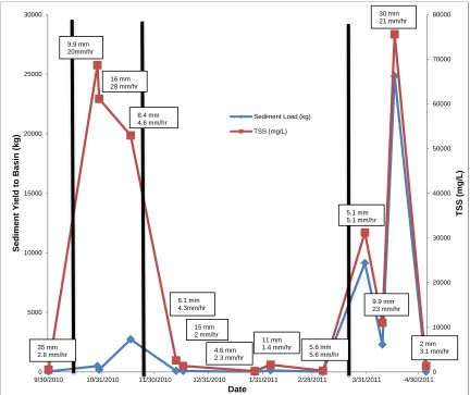
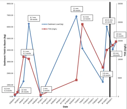
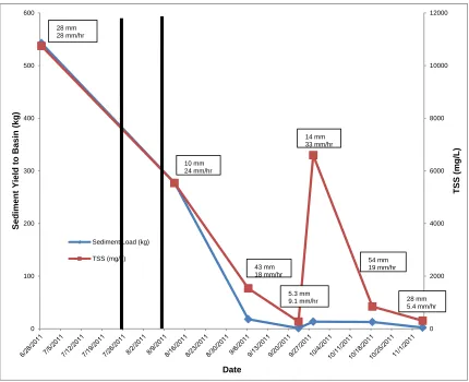
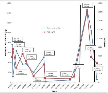
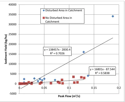
Figure 3-8. Sediment Yields and TSS from each storm collected on Basin 5.10 B. The points indicate a rain event with the boxes displaying rainfall depth and intensity from the storms. The left most box correlates to the left most point(s), etc. Lines were placed at specific dates of major grading and management events. ... 44 Figure 3-9. Graph of the independent variable, peak flow, and dependent variable, sediment yield per unit area (kg/ha), with equations of regression lines show the

(35)

Figure 4-4. RUSLE2 sediment yield estimates plotted against the difference between the field and RUSLE2 sediment yields ... 89 Figure 4-5. Plotted storms with field sediment yield and RUSLE2 calculated sediment yield on an individual basis. ... 90 Figure 4-6. Cook’s D test plot. Those points above the horizontal line are considered to be outliers. ... 93 Figure 4-7. Comparison of sediment yields calculated by RUSLE2 in tons as the

topography of the catchment for Basin 11.4 B changes. ... 98 Figure 4-8. Comparison of sediment yields calculated by RUSLE2 in tons as the

topography of the Basin 9.2 C changes over time. ... 101 Figure 4-9. Comparison of RUSLE2 estimates of sediment yield over time as

topography changes, and to planned estimates for Basin 10.3 B... 103 Figure 4-10. Comparison of the RUSLE2 sediment yield estimate over time as

(36)

Figure A2-3. Photograph from 9.14.10 when the survey was taken on Basin 11.4 B. The orientation of the photograph was looking up into the catchment near the basin’s location. ... 120 Figure A2-4. GIS processed survey from basin ID 11.4 B on 11.30.10 ... 121 Figure A2-5. Photograph from 11.30.10 when the survey was taken on Basin 11.4 B. The orientation of the photograph is looking up into the catchment from the location of the basin’s location. A fill pile (center, where total station set up is located in the

photograph) was moved into catchment. There was some grading in the center of the catchment, but not dramatic. The entire area was strawed and tacked with no

(37)

(38)

basin. The entire area had cover (mulch, wood chips, or straw) with limited grading or topography changes from the original grade. ... 135 Figure A2-19. GIS processed survey from basin ID 9.2 C on 06.08.11 ... 136 Figure A2-20. Photograph from 6.08.11 when the survey on Basin 9.2 C was taken. The orientation of the photograph is looking up into the catchment taken at a location near the inlet of the basin. There was limited change to the cover and topography since the previous survey was taken. A small portion at the top of the catchment had

(39)

Figure A2-26. Photograph from 6.8.11 when the survey on Basin 10.3 B was taken. The orientation of the photograph is looking up into the catchment from a location near the inlet of the basin. The entire area was strawed and tacked. The catchment was at final grade when monitoring began. Notice on the left side of the photograph, a

(40)

pictured in the right center. The topography was nearly the same as the original grade where the only difference was a haul road located at the toe of the hill at the back of the catchment. The entire area was strawed and tacked with some vegetation growth. ... 149 Figure A2-33. GIS processed survey from basin ID 5.10 B on 11.14.11 ... 150 Figure A2-34. Photograph was taken on 11.14.11 when the survey on Basin 5.10 B was taken. The orientation of the photograph is looking up into the catchment at a location near the inlet of the basin. Little had changed in the catchment in terms of cover and topography except for a fill pile on the left side using this orientation. ... 151 Figure A2-35. Photograph was taken on 11.14.11 when the survey on Basin 5.10 B was taken. Based on the orientation of the photograph in figure A2-34, this is the left side of the catchment. This fill pile was located here from approximately 11.14.11 to 11.28.11 and no rainfall events occurred during this period. ... 152 Figure A2-36. GIS processed survey from basin ID 5.10 B on 12.13.11 ... 153 Figure A2-37. Photograph from 12.13.11 when the survey on Basin 5.10 B. The

(41)

(42)

(43)

CHAPTER 1: LITERATURE REVIEW

1.1 Erosion on Construction Sites: The Effects and Regulations

With the rapid growth and development of cities, the amount of construction for an area will increase at least to some degree. Most of these construction projects involve a high level of disturbance and periods of disturbed and exposed soil surfaces to the land which makes the soil highly susceptible to erosion. In recent decades there has been an increase in the number of regulations concerning erosion control from construction sites and for good reason. Wolman and Schick (1967) found that with every increase of 1000 people to a city or town, the sediment yield from the construction that occurs as a result is estimated between 700 and 1800 tons. The amount of sediment discharged from a construction site can be on the order of 20 times greater than that yields from agricultural lands (Daniel et al., 1979). Due to this increased sedimentation in the receiving streams, there can be changes in biodiversity and populations which can result in long-lasting effects on the ecosystem naturally in place before construction (Barton, 1977; Taylor and Roff, 1986). Furthermore, since the stormwater systems are typically installed on a construction site early in the

(44)

In compliance with the Clean Water Act, the Sedimentation Pollution Control Act of 1973 was passed (North Carolina General Statutes, 2002). The act established for land disturbing activities, permits would be required and in order to obtain a permit an erosion and sediment control plan is needed and the plan is required to be followed through the

progression of the project. More recently, the US-EPA has attempted to establish an average turbidity discharge required on construction sites, that is for discharges from a site from storms less than a 2-year, 24-hour frequency, the average turbidity level must be below 280 NTU (Code of Federal Regulations, 2011). However, because of known errors in calculating the required average turbidity level and lawsuits from various contractors and groups, the passing and enforcement of the regulation has been delayed (Roder, 2011; US-EPA, 2010). The proposal for the average turbidity discharge limit is being looked into further taking into consideration the desires of the different building groups as well as a larger database.

1.2 Planning For and Controlling Erosion

Sediment basins are a commonly used best management practice (BMP) option for controlling and minimizing the amount of soil coming off of road and highway construction sites in North Carolina. Research has shown that the levels of total suspended solids (TSS) coming off of a construction site are variable and highly dependent on the site itself (Daniel et al., 1979; McLaughlin et al., 2009). Due to the usually simplistic methods for designing sediment basins, many of the basins used on highway construction sites may be over- or under-sized for the particular drainage area.

(45)

cover (Toy et al., 1999). On a construction site, the topography and land cover can change from day to day based on the stage of construction they are currently working. It is not uncommon for the catchment that a sediment basin is treating to have the cover, topography, catchment size, and potentially the soil type to change throughout the progression of the project. The different locations, and more importantly the different climates at those locations, have different intensities and frequency of rain as well as freezing and thawing cycles that can have dramatic effect on the amount of sediments being eroded (Foster et al., 2003). The texture of the soils affects the erodibility of them with silty soils being the most susceptible (Foster et al., 2003). The topography affects the level of erosion because of the length and steepness of a slope, but also the sediment yields and the enrichment of the soil texture due to concave sections within the topography. These areas will cause some larger particles to settle out and deposit (Foster et al., 2003). Alternately, when compared to a constant average slope a convex slope can yield more sediment. With there being a

difference in almost all of these factors between construction sites and there being multiple factors influencing soil erosion, there would never be a direct relationship between a few design parameters and the amount of sediments coming from the site.

(46)

1.3The Evolution of USLE

From the USLE, further research stemmed to be able to apply the equation to non-agricultural lands. With the advent of computers and the complicated and tedious

calculations that are required by the equation as more factors were taken into account, it was integrated into a texted based computer program aptly named the revised universal soil loss equation (RUSLE) (Renard et al., 1997). As further progression in computing technology, further research in areas crucial to computing soil loss, and as weaknesses emerged from the first revision of the universal soil loss equation (USLE), the equation was developed into RUSLE2 (Foster et al., 2003). The framework of RUSLE2 is still rooted in the empirical relationships originally developed by USLE. The equation structure used in RUSLE2 is similar to that of USLE and RUSLE using a similar framework equation (1.1).

𝑎𝑖 =𝑟𝑖𝑘𝑖𝑙𝑖𝑠𝑐𝑖𝑝𝑖, [1.1]

(47)

Toy et al., 1998). Along with these improvements, there were also changes to the interface including a graphical windows based interface of the slope, the ability to input complex slopes, and the ability for it be used in every scenario where erosion would occur due to exposed soil and where runoff occurs due to the rainfall intensity being greater than the infiltration rate of the soil (Foster et al., 2003).

More recent developments include a friendlier construction planning look with accurate terms for construction managements and an accounting period function where the user can input a specific time period for soil loss. This, for instance, to be used with a

municipality’s rules regarding erosion control period to estimate soil loss in terms of tons per acre rather than on an annualized basis (Yoder et al., 2007). A method of including the runoff from a series of representative rainfall events was also added to RUSLE2 (Dabney et al., 2010). RUSLE2 does not generate runoff values since plot scale data suggested a higher correlation between intensity and erosion than runoff volume and erosion. Due to this, the Annualized Agricultural Non-Point Source Pollution Model (AnnAGNPS) (Binger and Theurer, 2001) was used to generate sets of rainfall and runoff information using the 30-year monthly mean climate data within RUSLE2. The rainfall and runoff data generated was included to provide a link, in the future, to estimating soil losses through gully erosion through the use of process based models such as the Chemicals, Runoff, and Erosion from Agricultural Management Systems (CREAMS) model (Foster et al., 1980 a,b).

RUSLE2 has been seen as a premier tool for soil erosion estimation. This is because of the availability of the program itself, as it is free for use by the public, and the

(48)

managements common on construction sites, and conservation practice data for use in the program that can make it applicable to almost any situation, anywhere. Furthermore, since the foundation of the program is in the empirical development of USLE and the 10,000 plot years of research data, it is very robust as far as erosion estimation equations are concerned (Yoder et al., 2007). RUSLE2 can also be easily changed which provides a quick look at different erosion control scenarios for a fast determination of the most effective and appropriate plan.

Even with its validation and large data set used to create the program, the results can be highly varied from the actual sediment yields on a modeled site. The authors of RUSLE2 note that the sediment yield estimates from the program can be larger or smaller than the actual field yields by fifty percent (USDA NRCS, 2003). The authors further emphasize the fact that RUSLE2 may have inherent errors, should be used to assist in erosion control planning, and professional judgment should also be used in the interpretation of the results (USDA-ARS, 2008).

(49)

review of erosion from constructions sites. There was no field verification of the values obtained through RUSLE2.

The program was also used on a Pennsylvania interstate highway construction site and compared to volumes of sediment deposited in basins and to grab sample concentrations of TSS collected at the inlet and outlets of those basins (Kalainesan et al., 2007). The study found that RUSLE2 produced values 25% to 30% greater than what was found through field samples. Although, it was noted that the concentrations coming out of the basins were greater than the concentrations going in to the basins due likely to the fact that the basins were not maintained well or filled faster than the rate at which they were designed to fill. The only information the authors concluded was that there is a great need for a process based model to be implemented to calculate sediment basin size so they do not fill faster than they are supposed to and that BMPs on construction sites need to be maintained properly. The implications and conclusions of this study are limited due to the suspect methods in calculating sediment yields and the use of BMPs in RUSLE2.

Similar to the case earlier in Wisconsin, RUSLE2 was used to model erosion from natural gas well sites (Wachal et al., 2008). The author modeled a number of different BMP scenarios in the program to evaluate the cost-benefit of certain BMPs as well as combinations of BMPs. But like the scenario in Wisconsin, no field verification of the program was

(50)

be used on a multitude of situations as a means of developing erosion and sediment control plans.

Caltrans (California’s Department of Transportation) has begun to incorporate RUSLE2 into its erosion control plan as a means of estimating the amount of sediment to expect from a site and to be able to test the best method of how to limit rates of erosion (Caltrans, 2008). Caltrans used the RUSLE2 originally developed by the USDA-ARS and made modifications to some of the inputs and interface options to change and remove pieces in order to move the program away from something geared toward agricultural soil

conservation to a program more applicable to soil conservation on a construction site. The modifications included additions of cover, climate, and soils, as well as modifications to the vernacular of the management/operation options so engineers using the program will

accurately describe the processes occurring on the site. This ensures less misuse of the program and therefore more accurate estimations of soil loss. While this is a significant step to incorporate the program into erosion control plans, it was more so a modification to ensure the program was used correctly, and therefore there is still a need to see if the program is flexible and accurate to be able to model the levels of erosion coming from a construction site.

The North Carolina’s Department of Transportation (NCDOT) currently uses RUSLE2 in estimating soil loss on some projects including road widening projects,

(51)

bulk density of the soil found by the soil survey and multiplied against the constant 32.02 to convert the units from g/cm3 to tons/ft3. The area disturbed is then multiplied against this value and used as the storage volume necessary for the erosion control device being used (RUSLE2 Guide, 2009). This approach assumes no influence of sediment erosion from channelized flow, and assumes all sediment entering into these basins settles out in them.

1.5Gully Erosion

RUSLE2 does not model gully erosion. This poses a significant problem when using RUSLE2 for estimating sediment yields from construction sites since it is common practice to channelize flows in silt ditches to direct stormwater into basins, and that ephemeral gully erosion can have a dramatic impact on the total sediment yields on a catchment (Dabney et al, 2010). Posen et al. (2003) has highlighted the great need for research in this area. Understanding, estimating, and predicting how gully erosion will occur, how much it will contribute to the overall sediment loss from the catchment, and threshold levels as to where channelized flow will begin is a very complex issue. All of these pieces that define gully erosion depend on a variety of different factors including time, environment, soil pedology, hydrology, soil texture, climate, land management, etc.

The current models available for estimating gully erosion are limited, with the major ones being Chemical, Runoff, and Erosion from Agricultural Management Systems

(52)

the flow are transport capacities to carry the sediment some length downstream. The authors of these methods claim the models have valid predictions for soil erosion in gullies, but these models have not be through field testing in a wide range of conditions (Posen et al., 2003). Furthermore, these models cannot predict the start of a gully in the landscape; something left to the user to assess on a field visit for the catchment being modeled.

The effects of gully erosion in a catchment can be dramatic and should not be ignored when estimating soil erosion and sediment yields. The current research in the areas of large scale spatially and temporally is limited and needs to be expanded to aid in erosion

prediction.

1.6 Research Need

Even though the program itself is relatively robust in nature and the basis is the empirical relationships developed by 10,000 plot-years of data (Wischmeier and Smith, 1978), these models and equations are commonly misused by engineers, policy makers, and watershed modelers (Boomer et al., 2008). The model has been cited as being continually used to estimate soil loss in situations which were not originally researched in the

development of USLE. Such extrapolation of the data may lead to poor sediment yield estimates. Cover factors, topography changes, gully erosion, and other nuances on

construction sites have been cited to be very important and can have a significant change in the sediment yield predicted from a drainage area (Boomer et al., 2008).

(53)

and 325 square feet of surface area for every cubic foot per second of the peak flow off of the catchment for a ten year storm.

Using the logic presented here for designing a basin, there should be a linear

relationship between the sediment yield from a catchment and the area of the catchment, and a linear relationship between the sediment yield per unit area of the basin and the peak flow from a rain event. In the development of USLE, Wischmeier and Smith (1978) found that when all other factors were held constant, the erosion index (EI) had the most effect on sediment yields. The EI is essentially a measure of a storm’s intensity based on previous rainfall records. This suggests that sediment control structures should be designed based on the intensities of rain storms and not necessarily the volume of runoff from them. Since RUSLE2 uses this parameter when calculating the sediment yield estimate, the model will provide accurate and precise estimations of rill and interrill erosion.

The current regulations for designing sediment basins on highway construction sites are a simplification of what drives soil erosion taking into account only a few of the factors that impact sediment yields. By applying RUSLE2 and properly using the results, the

(54)

CHAPTER 2: SURVEYS AND CHANGES IN TOPOGRAPHY

2.1 Introduction

In a typical highway construction project, the topography of the catchment is changed dramatically during the course of construction. However, typically only the initial,

undisturbed and final design topographies are included in construction plans, so it is of interest to document the changes that occur between the beginning and end slopes and how that might affect the erosion in the catchment. This can be qualitatively analyzed by evaluating and comparing digital elevation models (DEMs) from surveys taken during the progression of grading in the catchment. The changes in topography can be quantitatively evaluated by comparing the average slope in the catchment of each survey and evaluating how much that influences the erosion and sediment yields during that portion of the project.

The objective of this portion of the research was to provide detailed

documentation of the changes to the topography on a typical highway construction site from the initial rough grade through the final grade. This was accomplished by using ground based light detection and ranging (LiDAR) to collect surveys on each of the basins with the exception of the first two surveys of Basin 11.4 B. These surveys were taken with a TopCon total station on 9/14/10 and 11/30/10. The points were exported and processed in a similar way as the data points from LiDAR.

(55)

being able to gather a LiDAR scan at the same point spacing every time. Any small

inconsistency such as removing extraneous points, taking a scan from a different position in the catchment, or reducing the point cloud grid spacing for processing in GIS is limited by the high level of precision and accuracy as indicated by the small point spacing that is obtained and be more accurate in tracking changes in the topography (Lokteff et al., 2011). The disadvantages of the system include the comparative cost, the extraneous points such as vegetation and machinery which have to be removed and block the view of any points directly behind, and shadowing effects that may result from the side orientation of the machine and contours in the catchment (Perroy et al., 2010).

The system has the position and distance accuracy of plus or minus six and four millimeters respectively for distances between 1 and 50 meters. The horizontal and vertical angle accuracy is plus or minus 60 microradians (Leica, 2007).

An attempt was also made to use the LiDAR to estimate the levels of erosion and deposition in the silt ditches. The intention was to take surveys periodically throughout the project of the silt ditches, and from those surveys a ‘flat’ surface could be created using only points outside of the ditch and compare it to a surface using all of the points. By comparing the two surfaces, the volume of the ditch could be found for a particular date and by

(56)

There are also technical issues surrounding this approach as well. The position of the LiDAR itself can create shadowing effects and therefore may alter the perception of the ditch when analyzing it for its volume. Perroy et al. (2010) found that the side looking orientation and limited footprint area provide limitations to estimating gully erosion. The authors also found this method for estimating erosion and deposition to be difficult as well, stating that the method was reasonable but could benefit from refinement and further research into this technique.

The purpose of the results documented in this portion of the thesis was to assess how the topography in the catchment changes as grading occurs through evaluation qualitatively of the surveys of the catchments and by analyzing how the average slope of the catchment changes, and make an evaluation on how the changes in average slope change the sediment yields to the basins.

2.2 Methods and Materials

2.2.1 Survey Techniques of Catchments

A ScanStation2 (Leica, 2009) was used to take ground based LiDAR surveys of the catchments for the basins. The ScanStation2 was generally set up near the same location on each basin site and set up to take surveys at point spacing between 0.05 m and 0.20 m. On Basins 11.4 B and 9.2 C multiple surveys were taken and combined because of the size of the catchments.

(57)

were combined with other scans and extraneous points (trees, machinery, vehicles, etc.) were removed. The remaining points were exported as a comma space delimited file to import to GIS for further processing.

2.2.2 Survey Post-Processing for Application to RUSLE2

All of the surveys for the catchments were processed in a similar way in ArcGIS 10 (ERSI, 2010). The X, Y, Z data were added to the workspace from a comma space delimited file and a boundary was created around the points and set as the mask. Within the spatial analyst tools, the inverted weighted distance (IDW) was used to develop a DEM. The DEM was then processed using the ‘fill’ function to smooth the contours. The ‘slope’ function was used on the fill layer to find the slope at points within the catchment. The flow direction was calculated using the filled DEM and then the flow accumulation was found using the flow direction layer. The flow length was then calculated using the flow direction. By creating a boundary around the catchment and setting it as a mask, the slope function was used again to create a slope layer where the average slope from which was used to compare the slopes from survey to survey.

2.2.3 Data Analysis

The information gathered was compared visually from survey to survey between basins and also quantitatively by using ArcGIS to calculate an average slope for the

(58)

highlighted in section 3.3.4. The stepwise function adds and removes variables from a regression model that could be used to predict dependent variables based on the independent variables based on a significance level of 0.15. In this case, if average slope were to be picked in the stepwise function, this would give evidence that the average slope of a catchment would have an impact on the sediment yields reaching the basin.

2.3 Results and Discussion

The surveys taken on each basin are shown in the processed form in figures A2-1 through A2-16 in the appendix. By a visual comparison of the surveys, it was typical that the areas went from smooth, natural hills to areas of minor and shallow slopes in the middle where a road bed would be built with steeper slopes on the side areas. During the course of the projects there were generally limited points when oddities such as temporary fill soil piles or cut areas with steep slopes were left in the catchment.

(59)

Figure 2-1. Points within catchment area taken with total station on Basin 11.4 B on 11/30/10.

(60)

The average density changed from 1.1 points per square meter when the total station was used on basin 11.4 B on 30 November 2010 to 20 points per square meter on Basin 11.4 B on 14 December 2010 when the LiDAR was used.

The average slopes from the processed surveys are displayed for each of the surveys taken on each basin in the tables below.

Table 2-1. Average slope in catchment of Basin 11.4 B for respective survey. Surveys taken with total station or LiDAR as noted.

Date of Survey Average Slope (%) 09/14/2010 (Total Station) 13

11/30/2010 (Total Station) 11.9 12/14/2010 (LiDAR) 11.6

2/3/2011 (LiDAR) 11.4

3/15/2011 (LiDAR) 13.3

4/25/2011 (LiDAR) 18.6

Table 2-2. Average slope in catchment of Basin 9.2 C for respective survey. All surveys taken with LiDAR.

Date of Survey Average Slope (%)

4/25/2011 9

6/08/2011 8.8

8/10/2011 7

(61)

Table 2-3. Average slope in catchment of Basin 10.3 B for respective survey. All surveys taken with LiDAR.

6/8/2011 4.5

8/10/2011 13.1

11/14/2011 13.5

Table 2-4. Average slope in catchment of Basin 5.10 B for respective survey. All surveys taken with LiDAR.

8/10/2011 16.4

11/14/2011 19.5

12/13/2011 13.6

From the average slopes from the surveys taken on each of the basins, there does not appear to be a pattern and for some cases the average slope is generally constant. The DEM for each survey with correlating pictures and catchment descriptions are in figures A2-1 through A2-37 in the appendix.

Based on the development of a regression equation using the stepwise function in SAS software, when all of the storms were analyzed together, average slope was not selected as significant (Table C2-1). When the storms were split among their respective basins, the sample sizes was too small for an appropriate analysis and average slope was not selected as significant for any of the basins when entered to the regression (Tables C2-2 through C2-5).

(62)

likely that there may be large amounts of erosion in steep sloping areas, but most of this sediment is deposited on flat grades before it reaches basins.

2.4 Conclusions

The use of LiDAR increased the density of the points dramatically from 1.1 to 20 points per square meter. By increasing the point density, the accuracy of the slope and distance between two locations of relatively close proximity is increased. This increased accuracy is accomplished in a shorter period of time and with less man-power than by using a total station.

The system can be set to take survey points of particular grid spacing, and therefore delivers a consistent scan of the catchment each time.

(63)

CHAPTER 3: Analysis of Sediment Yields and Basin Performance with Relation to Current Skimmer Basin Sizing Methods

3.1 Introduction

The increase in population of an area tends to lead to rapid construction and

development of housing and infrastructure which due to exposed soil surfaces can accelerate the rate of erosion from an area (Wolman and Schick, 1967). Allowing this sediment load to enter to streams and lakes can fill in these bodies of water and can affect the water quality impacting the biodiversity and benthic habitat of the water way (Barton, 1977; Taylor and Roff, 1986). Due to this, the Clean Water Act (33 U.S.C. 1251 et seq.) was passed by the United States Congress and subsequently the Sedimentation Pollution Control Act of 1973 was passed in North Carolina to establish a permitting system requiring sediment and erosion control plans for land disturbing activities (North Carolina General Statues, 2002).

Sediment basins are a common BMP used on construction sites. The sedimentation basins constructed on NCDOT sites are based on a few parameters having to do with the hydrology and sedimentology of the catchment the basin is treating. There are a wide variety of variables that have influence on the amount of sediment eroding and reaching a basin (Daniel et al. 1979; McLaughlin et al., 2009; Toy et al., 1999). This fact, along with the high level of change in the catchment and nuances typical of a highway construction project, a simple method for designing these sedimentation basins would not be a valid approach for ensuring good performance and control of sediment discharging from the site.

(64)

sensitive watersheds) for the basin volume and surface area. Sediment basins with surface outlet devices on highway construction sites require 126 cubic meters of storage space for every hectare disturbed and 1070 square meters of surface area for every cubic meter per second of the 10-year peak flow (or 25-year when applicable) (NCDOT, 2010). Since the storage volume is calculated based on the amount of disturbed area in the catchment, there should be a strong linear relationship between the sediment yields into the basin and the disturbed area in the catchment. Also, since the surface area is designed to ensure sufficient deposition in the basin and by relation efficiency of the basin, there should be a strong linear relationship between the peak flow and basin efficiency.

The objectives of this research were to:

• Measure sediment runoff concentrations and yields moving in and out of basins

during different phases of construction on a NCDOT highway development project.

• Evaluate current sediment basin design for basin performance and sediment loading

using storm event and management data from four disturbed catchments during all phases of highway construction.

• Identify appropriate design variables as better predictors of basin performance and

sediment yield during NCDOT highway development.

3.2 Methods and Materials

3.2.1 Sediment Basin Monitoring

(65)

were located in the Piedmont region on the I-540 extension construction project in Wake County, North Carolina.

The inlet and outlet of each basin were monitored with ISCO 6700 automated samplers (or ISCO 6712) with a 730 bubbler modules (ISCO, Inc., Lincoln, NE, USA) to measure the stormwater flow and collected samples on a volume weighted basis.

The standard inlet of a basin on NCDOT sites use a 30.5 cm corrugated plastic slope pipe drain (NCDOT, 2010). The bubbler tube and the sampling tube were glued into the inlet pipes. The length and average slope of the pipe was determined individually and the

samplers were programmed to internally calculate the flow rate using Manning’s equation and from that the volume of water that had passed for a specific period of time (ISCO, 2008). The samplers were programmed to collect a 200 mL sample of stormwater for a defined volume that had passed after reaching an enable level. The enable level was set to 1.06 mm which is the level of stormwater in the inlet pipe before sampling was initiated. Samples were taken after a known volume had passed (Tables 3-1 and 3-2), which was selected based on expected flows in each catchment and experience during the monitoring period.

Table 3-1. Volume of stormwater required to pass to initiate the collection of one 200 mL sample by the sampler at the inlet of each basin.

Basin ID Passing Volume (L)

11.4 B 1890

9.2 C Front 2840

9.2 C Side 1890

10.3 B 1890

(66)

Table 3-2. Volume of stormwater required to pass to initiate the collection of one 200 mL sample by the sampler at the outlet of each basin.

Basin ID Passing Volume (L)

11.4 B 1890

9.2 C 2840

10.3 B 945

5.10 B 2840

The samplers were programmed to collect four 200 mL aliquots per bottle, which would represent that portion of the hydrograph and sedigraph. Composite sampling allowed for more samples to be taken over the course of a storm, providing a better estimate of the true average TSS concentration over time.

A 1200 V-notch weir was installed near the outlet of the basins in order to measure the flow from the skimmer and emergency spillway. The flow over the weir was determined from the level given by the 730 bubbler module and the weir program in the sampler. Similarly to the inlet, samples were collected on a flow-weighted basis in four 200 mL aliquots per bottle.

An ISCO 674 Rain Gage (ISCO, 2008) was attached to one of the samplers to monitor rainfall depths to an accuracy of 0.254 mm and was assumed to represent the rainfall for other basins that were monitored on the project at the same time. The amount of rainfall was recorded every five minutes by the sampler.

(67)

After rain events, samples were collected and analyzed for total suspended solids (TSS) and turbidity. Every sample was analyzed for turbidity while the TSS was measured for every fourth sample due to time and expense.

Turbidity was measured using a TC-3000e portable turbidity meter (version 1.5, LaMotte, Chestertown, MD). The measured values were corrected with a standard curve based on a series of formulized standards. Following the Standard Methods for the

Examination of Water and Wastewater (Clesceri et al., 1998), TSS samples were filtered with 47 mm glass fiber ProWeigh filters from Environmental Express (Mt. Pleasant, SC) and dried overnight at 103°C to 105°C.

In order to obtain an estimate of TSS of each sample, a linear relationship between TSS and turbidity was developed for each site using the samples that were analyzed for both turbidity and TSS. The data were graphed with turbidity being the independent variable and TSS being the dependent variable. A regression equation was calculated based on the graphed data and used to estimate the TSS based on the turbidity for the other samples (Gippel, 1989). These graphs are displayed in figures C3-1 through C3-4 in the appendix.

Using the flow and time data, the representative volume that went into the basin during the course of when a sample was collected was calculated. By using the volume and the TSS of each sample, the mass of sediment entering the basin was calculated.

(68)

the basin for a specific storm (Tables C3-1 through C3-8). Other factors such as whether polyacrylamide (PAM) for flocculation was used, whether grading was occurring, and whether discharge occurred over the emergency spillway of the basin occurred were also recorded.

Spillway discharge was assumed when the outflow at the weir exceeded the

maximum flow rate of the skimmer, as provided by the manufacturer (J.W. Faircloth & Son, Inc., Hillsborough, NC).

For each storm where inlet and outlet samples collected, basin performance based on TSS, NTU, and total sediment were also calculated using equation 3.1.

𝐵𝑎𝑠𝑖𝑛𝑃𝑒𝑟𝑓𝑜𝑟𝑚𝑎𝑛𝑐𝑒 (%) =𝑉𝑎𝑙𝑢𝑒𝐼𝑛−𝑉𝑎𝑙𝑢𝑒𝑂𝑢𝑡

𝑉𝑎𝑙𝑢𝑒𝐼𝑛 ∗100% [3.1]

The storms which included inlet samples and inlet and outlet samples were compiled with the properties as described and put into tables 1 through 4 and 5 through C3-8 respectively. During some storms, low flows and malfunctions were recorded by the sampler and as a result, the data from these events were not used in the analysis.

The basins were monitored for as long as possible to estimate long term erosion rates for the catchments of the basins and to see how sediment delivery to the basins changes as the topography and groundcover in the catchment change through the project’s progression.

3.2.2 Site and Basin Descriptions

3.2.2.1-Basin ID 11.4 B

(69)

3-1) and was monitored from 9/14/2010 to 5/5/2011. The description of this basin and the design numbers are listed in table 3-3 and 3-4.

Table 3-3. Design dimensions and calculations for Basin ID 11.4 B for clearing and grubbing phase.

Design Property Value

Length (m) 29.0

Width (m) 12.2

Depth (m) 0.915

25-Year Peak Flow (m3/s) 0.315

Disturbed Area/Drainage Area (ha) 1.05

Intensity for Rational Method (mm/hr) 198

C-factor for Rational Method 0.55

Skimmer Orifice Diameter (mm) 41.3

Emergency Spillway Weir Length (m) 9.76

Table 3-4. Design dimensions and calculations for Basin ID 11.4 B for final grade phase.

Length (m) 29.0

Width (m) 12.2

Depth (m) 0.915

(70)

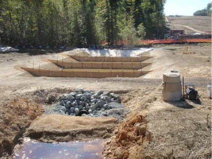
Figure 3-1. Basin ID 11.4 B

This basin was monitored from soon after its installation through the end of the clearing and grubbing phase and into the beginning of the mass grading phase for this portion of the project. Monitoring of this basin was terminated because of a majority of the sediment yield was originating from the silt ditch leading into the basin.

(71)

load from the catchment leading into 11.4 B, it would not be a valid comparison without subtracting out this extra sediment load.

The monitoring of 11.3 C ended on 02/03/11 when the basin was removed in accordance to the plans.

On the dates 9/14/10 and 11/30/10, surveys were collected with a Topcon Total Station (GTS 211D, Topcon Electronic Total Station, Livermore, CA) because of

malfunctions with the LiDAR scanner. The surveys for this basin were conducted and the data processed in ArcGIS as described in chapter 2. All surveys collected and processed on this basin are displayed in figures A2-2 through A2-7.

3.2.2.2-Basin ID 9.2 C

The inlet and outlet of basin ID 9.2 C (State Project Reference Number: R-2635A) east of Apex-Holly Springs Rd. (Figure 3-2), was monitored from 3/22/2011 to 9/16/2011. The description and design calculations for the basin are listed in table 3-5.

Table 3-5. Design dimensions and calculations for Basin ID 9.2 C for clearing and grubbing plans.

Length (m) 39.6

Width (m) 19.8

Depth (m) 0.915

(72)

Figure 3-2. Basin ID 9.2 C, view of front. Side inlet is to the left in the photograph.

Since there were two inlets on this basin, both inlets were monitored using automated samplers and the data combined to characterize flow into the basin. For description

purposes, the ‘front’ inlet was oriented parallel to the longest dimension of the basin, and the ‘side’ inlet was orient perpendicular to the longest dimension of the basin. This basin was monitored from the clearing and grubbing phase and through a portion of the mass grading phase.

(73)

sediment yield. On 6/14/2011, the ‘sumps’ typically dug out in front of rock check dams in the silt ditch were filled in and smoothed out, and jute fabric and wattles were installed to limit erosion. The soil deposited in front of the wattles and check dams was estimated by measuring the length, width, and depth of the deposits, and obtaining the bulk density to convert to the volume estimated to mass.

All of the surveys were conducted using LiDAR and processed in GIS as described in chapter 2, and are displayed in figures A2-8 through A2-11.

3.2.2.3-Basin ID 10.3 B

(74)

Table 3-6. Design specifications for Basin ID 10.3 B for final grade plans.

Width-Top (m) 9.15

Length-Top (m) 13.7

Depth-Top (m) 0.915

Width-Bottom (m) 9.15

Length-Bottom (m) 13.7

Depth-Bottom (m) 0.915

Disturbed Area/Drainage Area (ha) 0.769 Intensity for Rational Method (mm/hr) 198

Emergency Spillway Weir Length (m) 6.71

(75)

This section of the project was at final grade and it wasn’t anticipated that much grading would occur and therefore most of the sediment movement would be a result of erosion.

All of the surveys were conducted using LiDAR and processed in GIS as described in chapter 2, and are displayed in figures A2-12 through A2-14.

3.2.2.4-Basin ID 5.10 B

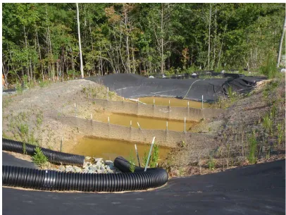
The inlet and outlet of basin ID 5.10 B (State Project Reference Number R-2635A; Figure 3-4) was monitored from 8/4/2011 to 12/16/2011. This basin was located west of the NC 55 by-pass near Holly Springs, NC. The description and design calculations for the basin are listed in table 3-7.

Table 3-7. Design dimension and calculations for Basin ID 5.10 B from clearing and grubbing plans.

Length (m) 24.4

Width (m) 12.2

Depth (m) 0.915

Disturbed Area/Drainage Area (ha) 0.708 Intensity for Rational Method (mm/hr) 198

(76)

Figure 3-4. Basin ID 5.10 B

In order to limit channel and gully erosion, the silt ditches leading to this basin were lined with Posi-Shell (Posi-Shell, 2011). Posi-Shell is a mixture of water, fibers, a mineral setting agent, and Portland cement and which mixed and hydraulically applied, much like hydromulch. It is a very durable material and in theory should prevent in the silt ditches. Wattles were also installed in these ditches and the level of sediment deposition was

measured as described previously and subsequently removed by hand periodically. A sample was collected at the time sediment was removed for bulk density.

(77)

3.2.3 Data Analysis

The properties for each storm were analyzed by calculating Pearson’s correlation coefficient and constructing regression equations in SAS software (SAS, 2009).

The Pearson correlation coefficient was found between all possible combinations of the variables in the analysis simultaneously. The Pearson coefficient is a measure of the association between two variables and can range from -1 to 1 where a coefficient of 1 implies a perfect positive relationship between the dependent and independent variables. A

correlation coefficient of -1 implies a perfect negative relationship between the two. From the coefficient, a probability could be found and used to establish whether the correlation between the two variables was significant. Any of the correlation coefficients with a p-value lower than 0.05 were considered significant.

A model regression between one variable or multiple variables was constructed. In other words, a model was constructed to find which of the independent variables had a

significant (p ≤ 0.05) influence in predicting the dependent variable. This was done using the

stepwise functions.