Development of Simulation Methodology to Predict Crack Growth Behavior in Heavy Duty Truck Components using Full Vehicle Response Dynamic Loads.

ABSTRACT

RAO, VINAY NAGARAJA. Development of Simulation Methodology to Predict Crack Growth Behavior in Heavy Duty Truck Components using Full Vehicle Response Dynamic Loads. (Under the direction of Dr. Jeffrey W. Eischen.)

This dissertation develops a novel simulation methodology for three dimensional fretting and mixed mode fatigue crack growth problems using full vehicle dynamic response of a heavy duty truck obtained during accelerated endurance testing of the vehicle. The typical product development simulation process used in the automotive/trucking industry does not identify fretting fatigue and crack growth behavior. This prevents identifying optimal design and root cause for fracture. This research helps to close the gap between damage tolerant and safe-life approaches by including fracture mechanics principles during root cause investigation and design development simulation process.

Failures in heavy duty truck frames typically involve crack growth under mixed mode I/II/III loading since the dynamic vehicle loads are highly nonlinear transient and multi-axial with large deformation behavior. It is critical that propagation of cracks in truck frame members be well studied since on reaching critical crack lengths they can lead to complete breakdown of the vehicle and this may lead to catastrophic accidents with loss of life. Although there are routine vehicle inspections to detect and repair / replace fatigue cracked components, the ability to better predict crack path and orientation under various loading conditions can help avoid expensive losses and improve the design with better durability.

simulation on the component level model using dynamic interface loads. The large computational time of the simulation process was reduced by identifying critical load events (load sensitivity study) causing failure, and further reducing the critical load events to retain only the damage causing sections for crack growth simulation.

In this research a combination of FRANC3D (3D crack growth simulation program [7]), NASTRAN (finite element solver [41]) and multiple programs (fatigue solver, signal processing program, batch scripts) were used and semi-automated to determine stress intensity factors, crack orientation and number of cycles to grow the crack. The simulation results obtained in this dissertation provide good agreement with physical test results for all the case studies reviewed.

Development of Simulation Methodology to Predict Crack Growth Behavior in Heavy Duty Truck Components using Full Vehicle Response Dynamic Loads

by

Vinay Nagaraja Rao

A dissertation submitted to the Graduate Faculty of North Carolina State University

in partial fulfillment of the requirements for the degree of

Doctor of Philosophy

Mechanical Engineering

Raleigh, North Carolina 2016

APPROVED BY:

_______________________________ _______________________________ Dr. Jeffrey W. Eischen Dr. Eric C. Klang

DEDICATION

BIOGRAPHY

ACKNOWLEDGMENTS

I am greatly indebted to Dr. Jeffrey W. Eischen for being my advisor during my Ph.D. research work. He has helped me over the years understand the research area and encouraged me to stay focused and motivated. I thank the committee members, Drs. Eric C. Klang, Kara Peters, and John S. Strenkowski for their valuable suggestions and comments. I also thank Volvo Trucks North America for the financial support and consideration for my studies.

TABLE OF CONTENTS

LIST OF TABLES ... vii

LIST OF FIGURES ... viii

1. Introduction...1

1.1 Motivation...3

1.2 Scope of Research...4

1.3 Thesis Outline...5

2. Background...7

2.1 Extended Finite Element Method...7

2.1.1 Advantages and Limitations of X-FEM Method...9

2.2 Explicit Crack Front Re-Meshing Method...10

2.2.1 FRANC3D Methodology...12

2.3 Fretting Fatigue Crack Growth...15

2.4 Mixed Mode Crack Growth...21

2.5 Crack Growth Simulation Process...27

2.5.1 Fatigue Crack Growth Rate Model...31

2.5.2 Fracture Criteria...33

2.5.2.1 Maximum Tensile Stress Criteria...34

2.5.2.2 Maximum Shear Stress Criteria...35

2.5.2.3 Maximum Strain Energy Release Rate Criteria...36

3. Chassis Vehicle Dynamics...37

3.1 Frame Material Data...39

3.2 Finite Element Modelling...41

3.3 Boundary Conditions...44

3.4 Endurance Testing of Vehicles...46

3.5 Simulation Process...49

4. Proposed New Simulation Methodology...53

5. Case Studies...60

5.1 Fretting with Cylindrical Pads...60

5.2 Fretting with Square Indenter...65

5.3 Mixed Mode Crack Growth...70

5.4 Frame Fretting Fatigue Failure and Simulation...74

5.4.1 Simulation Results and Discussion...78

5.4.2 Multiple Crack Initiation Effect...85

5.4.3 Optimal Design Identification...87

5.5 Frame Mixed Mode Crack Growth...95

5.5.1 Simulation Results and Discussion...98

5.5.2 Sensitivity Analysis of Frame Open-Hole Location...105

6. Conclusions and Future Work...110

6.1 Validation of Simulation Methodology...111

6.2 Future Work...112

REFERENCES...114

APPENDIX...121

Appendix A – Bolt and Contact Definition NASTRAN Cards...122

Appendix B – NASTRAN Input for Enforced Displacement Analysis...126

Appendix C – Simulation Automation Program...128

LIST OF TABLES

Table 3.1: Monotonic properties for ASTM A322 Grade 4135...39 Table3.2: Low cycle fatigue Manson-Coffin model for frame rail material...39 Table 3.3: Fatigue crack growth results for frame material under different hole making process...40

Table 3.4: Charpy impact results for heat treated frame rail...41 Table 5.1: Frame rail tensile properties and hardness...74 Table 5.2: Design iterations considered for identifying optimal frame reinforcement solution...88

LIST OF FIGURES

Figure 1.1: Proposed analysis approach for full vehicle durability and root cause analysis

investigation... 2

Figure 2.1: Enriched nodes used in X-FEM... 8

Figure 2.2: Slightly eccentric crack in a cantilever beam... 9

Figure 2.3: Crack path evaluation for a plate with crack emanating from the edge of a hole (a) Experimental result (b) Crack growth simulation using finite element analysis...11

Figure 2.4: Fan Blade attachment in a typical gas turbine engine (a) Dovetail AFT face (b) Crack propagation with a corner flaw in FRANC3D...11

Figure 2.5: Crack growth analysis workflow with FRANC3D...13

Figure 2.6: Crack front element – Penta15 element with quarter points...14

Figure 2.7: Fretting fatigue setup illustration...16

Figure 2.8: Fretting test using universal servo-hydraulic fatigue machine (a) Double bolted lap joint specimen (b) Fretting wear obtained in test...19

Figure 2.9: Fretting map... 20

Figure 2.10: Mixed mode crack growth simulation (a) Plate with two cracks from drilled holes (b) Experimental and simulated crack path...22

Figure 2.12: Crack growth simulation with different initial crack angles in a plate subjected

to mixed-mode loading...26

Figure 2.13: Typical crack growth simulation process with explicit crack front re-meshing method... 28

Figure 2.14: Schematic of crack extension method...30

Figure 2.15: FRANC3D sub-modeling approach...30

Figure 2.16: Schematic illustration of the definition of the kink angle...33

Figure 2.17: Fracture locus using mode I and II stress intensity factors...34

Figure 3.1: Frame ladder location and configuration (a) Frame ladder in a full vehicle model (b) Typical Class 8 frame ladder and cross-member locations...37

Figure 3.2: Frame section (a) Frame web section, lower flange and upper flange (b) Frame sectional property dimensions...38

Figure 3.3: Payload modeling in a full vehicle model (a) Load rack representation (b) Trailer with trailer suspension representation. ...42

Figure 3.4: Shocks and suspension modeling in a full vehicle model (a) Shock absorber (b) Rear suspension for a tandem axle...43

Figure 3.5: Boundary conditions defined for transient response analysis of a full vehicle model...45

Figure 3.6: Simplified tire model (a) Tire model representation with spring-damper system (b) Full tire model with tire stiffness defined at tire-ground interface...46

Figure 3.8: Vehicle data acquisition from endurance test...48 Figure 3.9: Simulation process map typically used for full vehicle durability analysis and root cause investigation...49

Figure 4.1: Full-Vehicle response based 3D crack growth simulation process map...53 Figure 4.2: Contact definition between crack faces...55 Figure 4.3: Simulation automation process for fatigue analysis using full vehicle response loads...56

Figure 4.4: Load extraction in the area of interest using a rigid mesh...57 Figure 4.5: Simulation process used for creating enforced displacements from reduced loads...59

Figure 5.1: Fretting with cylindrical pads (a) Model setup (b) Displacement plot with crack growth (scaled displacement) ...61

Figure 5.2: Fretting fatigue simulation results (a) Stress plot with maximum stress along the contact trailing edge and at the mid-point of contact (b) Fatigue life plot indicating number of cycles to crack initiation...62

Figure 5.3: Fretting crack growth results with cylindrical pads (a) Crack growth model and simulation result after 8 iterations. (b) Experimental crack growth observed...63

Figure 5.4: Stress intensity factors plotted with crack growth steps for fretting using cylindrical pads...65

Figure 5.6: Fretting fatigue simulation results (a) Stress plot with maximum stress along the contact leading edge (b) Fatigue life plot indicating number of cycles to crack initiation...67

Figure 5.7: Fretting crack growth results with square indenter (a) Crack growth model and simulation result after 7 iterations. (b) Experimental crack growth observed...68

Figure 5.8: Stress intensity factors plotted with crack growth steps for fretting using square indenters...69

Figure 5.9: Mixed mode crack growth (a) Model setup (b) Displacement plot with crack growth (scaled displacement) ...70

Figure 5.10: Mixed mode crack growth results (a) Crack growth model and simulation result after 30 iterations. (b) Experimental crack growth observed...72

Figure 5.11: Crack growth model after 12 iterations and shear stress plot showing interacting stress zone...73

Figure 5.12: Stress intensity factors plotted with crack growth steps for mixed mode crack growth from two off-centered cracks...73

Figure 5.13: Frame fatigue crack observed (a) Crack observed on outer surface of frame during endurance test, (b) Section of the crack surface showing shear lip location...75

Figure 5.14: Fretting induced wear seen below central bolt hole on frame...76 Figure 5.15: Optical micrograph of the cross sectioned frame fracture...77 Figure 5.16: Magnified view of the fracture initiation site, contact wear visible along initiation site...77

Figure 5.18: Crack Insertion using FRANC3D (a) FRANC3D local model with semi-elliptical surface crack inserted (b) Semi-semi-elliptical crack as visible through the thickness...80

Figure 5.19: Frame crack growth simulation result (a) A small surface semi-elliptical crack initiated in the area of high fretting damage (b) Crack growth obtained after 6 steps of simulation run...81

Figure 5.20: Crack growth steps showing crack extension on frame under wireframe view...82

Figure 5.21: Stress Intensity factors plotted against crack extension on frame...83 Figure 5.22: Frame deflection and crack opening mode (a) Reverse bending of frame in side- view (b) Crack opening under reverse bending (Step 6 result) ...83

Figure 5.23: Simulation result comparison (a) Current simulation result done without 3D solid model and contacts (b) Simulation result using proposed methodology...84

Figure 5.24: Multi-crack insertion and stress intensity factors (a) Multiple cracks (Front, Center and Rear) inserted in fretting zone (b) Maximum stress intensity factors measured for inserted cracks...85

Figure 5.25: Multi-crack growth and stress intensity factors (a) Crack growth obtained after 3 steps (b) Maximum stress intensity factors measured for cracks...86

Figure 5.26: Baseline frame reinforcement description (a) Rectangular inner frame reinforcement plate (b) Pear shaped outer frame reinforcement plate...87

Figure 5.28: Contact configurations (a) Flat ended with sharp edge contact (b) Flat ended with rounded edge contact...90

Figure 5.29: Pressure distribution for a flat indenter with rounded corners (b/a =

0.0,0.1,…,1) ...91

Figure 5.30: Comparison of shear stress plot for frame articulation event (a) Baseline design (b) Optimal design with extended inner reinforcement...92

Figure 5.31: Comparison of fatigue damage plot (a) Baseline design with high damage in fretting zone (b) Optimal design solution with large Improvement in fatigue life...93

Figure 5.32: Stress intensity factor comparison between baseline and design solution having extended inner reinforcement...94

Figure 5.33: Failure investigation during endurance testing of the vehicle (a) Frame cracks visible near torque rod connection (b) Crack path visible on frame behind outer reinforcement plate...95

Figure 5.34: Crack path and crack origins on failed frame section (a) Complete crack propagation directions on frame section (b) Failure origin on analysis...96

Figure 5.35: Fractographic analysis of failed frame section (a) SEM image showing beach marks (b) Optical micrograph showing cracks on the wall of open-hole...97

Figure 5.36: Frame 3D solid sub-model used in crack growth simulation (a) Frame inner section view and description (b) Frame outer section view and description...98

Figure 5.38: FRANC3D crack insertion type selection (a) Surface elliptical crack inserted at edge of open-hole in FRANC3D (b) Crack front visible in wireframe view of open-hole...100

Figure 5.39: Crack growth steps showing crack extension on frame...101 Figure 5.40: Frame deformation during turning event (a) Out-of-plane bending of frame section (b) Crack opening under frame bending loads...102

Figure 5.41: Comparison of frame crack obtained during full vehicle endurance test with crack growth simulation result...103

Figure 5.42: Simulation result comparison (a) Current simulation result done without 3D solid model and contacts (b) Simulation result using proposed methodology...103

Figure 5.43: Stress Intensity factors plotted again crack extension on frame...105 Figure 5.44: Location of frame open-hole moved along “X” direction for sensitivity

study...106

Figure 5.45: Variation of stress magnitude depending on the distance of open-hole from its initial position...107

Figure 5.46: Stress variation and strain-life curve (a) Stress magnitude vs Distance of open-hole from its initial position (b) strain life curve for frame material...107

1.

Introduction

The product development of heavy duty truck components requires full vehicle durability analysis and testing for loads representing the vehicle usage pattern by customers. The full vehicle endurance test comprised of many dynamic test track events will identify any product design issues and the prior durability simulation (finite element analysis and fatigue calculations) of the full vehicle should be capable of predicting failure and design performance before testing. This is the general simulation standard required in the automotive and trucking industry. However often there is a lack of good agreement between simulation results and experimental failure in particular for heavy duty truck engineering.

Failures in heavy duty truck frames typically involve crack growth under mixed mode I/II/III loading since the dynamic vehicle loads are highly nonlinear transient and multi-axial with large deformation behavior. It is critical that propagation of cracks in truck frame members be well studied since on reaching critical crack lengths they can lead to complete breakdown of the vehicle and this may lead to catastrophic accidents with loss of life. Although there are routine vehicle inspections to detect and repair / replace fatigue cracked components, the ability to better predict crack path and orientation under various loading conditions can help avoid expensive losses and improve the design with better durability.

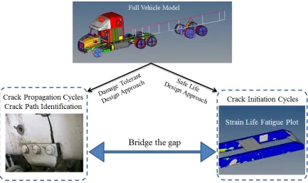
vehicle durability and root cause analysis simulations are computationally very intensive and complex process involving multiple simulation programs. This research was focused towards improving current simulation methods and to provide better correlation between test failure and analysis predictions. Figure 1.1 shows a schematic representation of the analysis approach that will enable applying fracture mechanics principles during root cause investigation of test failures in heavy duty trucks.

Figure 1.1: Proposed analysis approach for full vehicle durability and root cause analysis investigation

cracks in a design are considered as failure hence the simulation methods used for product development does not usually use fracture mechanics principles. However when the safe life approach was applied for failure investigation involving cracks, simulation methods does not explain the root cause and fails to provide an optimal solution. Damage tolerant approach considers cracks and crack growth behavior in product design. It is often required during failure analysis to identify crack propagation path, number of cycles taken to grow a crack for certain length and critical loads causing crack growth. The goal of this research was to combine both approaches during root cause investigation. A novel simulation method for failure investigation was developed to predict crack growth behavior in heavy duty truck components using full vehicle response dynamic loads.

1.1

Motivation

The application of advanced simulation methods and fracture mechanics principles using an optimal simulation methodology to support root cause investigation was not found in the literature. The main motivation of this research was to,

a) Develop a new simulation methodology for computationally intensive full vehicle durability analysis and predict accurate crack growth behavior in heavy duty truck components.

c) Improve agreement between test failures and simulation results so as to close unresolved / unknown issues causing quality letdown.

d) Avoid loss of operational time due to failures by improving product durability. Any loss of operational time of a machine / vehicle is often very expensive (both in repair cost and liability cost)

e) Improve product durability by providing advanced simulation results upfront during early product development stage.

f) Improve confidence in using simulation methods for resolving root cause investigations.

Motivation of this research is also driven by the fact that many test failures often are resolved in an ad-hoc manner without proper knowledge of failure mode and crack propagation behavior. Identifying crack initiation and crack propagation behavior will help avoid making costly repairs and provide optimal solutions.

1.2

Scope of Research

finite element models using NASTRAN solver. The full vehicle model dynamic response was used for crack growth study on a high fidelity component level model (contact definitions, pre-tension conditions and parabolic mesh refined to small element sizes) and the simulation process was semi-automated with multiple programs and scripts. The case studies were solved using proposed simulation process to identify crack initiation cycles, crack propagation path and critical loads causing failure. These results were compared to the reported experimental data to show good correlation, thus validating the proposed simulation methodology.

1.3

Thesis Outline

This dissertation was organized as follows:

The first part provides a brief introduction to this research, which includes the motivation, scope of research and an overview of the research objectives.

The second part provides literature background for this research, which includes extended finite element method (X-FEM), explicit crack front re-meshing method with FRANC3D program as example, fretting fatigue, mixed mode crack growth and crack growth simulation process with explanation for different fracture and crack growth criteria. The typical crack growth simulation process using an explicit crack front re-meshing method was also described.

current simulation process. The drawbacks and limitations of current simulation process were also highlighted. The finite element modeling details highlighted the meshing features, element types and modelling assumptions used in a full vehicle model.

The fourth part provides detailed explanation of proposed simulation methodology, which includes description of finite element models used, contact definitions, format conversion, automation, batch processing, multiple programs and scripts written to automate and enable crack growth simulation using FRANC3D program and NASTRAN finite element solver.

The fifth part provides detailed explanation of the simulation method and results obtained for five different case studies using proposed simulation method. The case studies were organized from simple fretting and mixed mode cases discussed in literature to more complex real endurance test failure of frame rail in heavy duty trucks. The simulation processes were validated for each of the case study by comparing to the reported experimental data.

2.

Background

A review of literature sources that cover the area of crack growth simulation using the extended finite element method and explicit crack front re-meshing method, fretting fatigue and mixed mode failure are explained in this section.

2.1

Extended Finite Element Method

In the XFEM ([1-3]) method it is not necessary to generate a mesh that conforms to the crack boundaries to account for the geometric discontinuity. It includes crack-tip enrichment functions and Heaviside enrichment for the nodes whose support is cut by the crack (and does not include the crack tip). Nodes whose support includes the crack-tip are enriched with eight additional degrees of freedom i.e., four crack-tip functions Fj(x) times the two directions of the domain space. Heaviside enriched nodes are with two additional degrees of freedom, one for each direction of the domain space. Figure 2.1 shows mesh portion of a fretting model, where the enriched nodes are marked [1]. Crack tip functions are given as,

𝐹𝐹𝑗𝑗(𝑟𝑟,𝜃𝜃) =√𝑟𝑟 �𝑠𝑠𝑠𝑠𝑠𝑠𝜃𝜃₂,𝑐𝑐𝑐𝑐𝑠𝑠𝜃𝜃₂,𝑠𝑠𝑠𝑠𝑠𝑠𝜃𝜃₂𝑠𝑠𝑠𝑠𝑠𝑠𝜃𝜃,𝑐𝑐𝑐𝑐𝑠𝑠𝜃𝜃₂𝑠𝑠𝑠𝑠𝑠𝑠𝜃𝜃� Eq. (1)

with j=1 to 4 and where (𝑟𝑟,𝜃𝜃) are polar coordinates of a local reference system with origin at the crack tip and aligned with the crack. The crack-tip functions constitute the basis functions that represent the first term of the LEFM displacement field, and consequently, reproduce the

For a 2D case, the XFEM approximation of the displacements at a point x of the domain is,

𝑢𝑢𝑥𝑥𝑥𝑥𝑥𝑥𝑥𝑥(𝑥𝑥) =∑𝑛𝑛𝑛𝑛𝑖𝑖=1𝑀𝑀𝑁𝑁𝑖𝑖(𝑥𝑥)𝑢𝑢𝑖𝑖 +∑𝑖𝑖=1𝑛𝑛𝑛𝑛𝐻𝐻𝑁𝑁𝑖𝑖(𝑥𝑥)𝐻𝐻(𝑥𝑥)𝑎𝑎𝑖𝑖 +∑𝑛𝑛𝑛𝑛𝑖𝑖=1𝐶𝐶𝐶𝐶𝑁𝑁𝑖𝑖(𝑥𝑥)�∑4𝑗𝑗=1𝐹𝐹𝑗𝑗(𝑥𝑥)𝑏𝑏𝑖𝑖,𝑗𝑗� Eq. (2)

Where nnM is the number of nodes in the mesh, and nnH, nnCT are the number of Heaviside and crack-tip enriched nodes, respectively. Ni(x), ui are the standard shape functions and standard degrees of freedom of each node i, respectively, and ai, bi,j are the additional degrees of freedom associated with the heaviside function H(x) and the crack-tip functions Fj(x).

Figure 2.1: Enriched nodes used in X-FEM [1]

X-FEM approach is implemented in FEA solver ABAQUS and successfully applied to 2D static and quasi-static crack growth problems by many authors [1], [2], [3].

In Figure 2.2, Giner et al. [2] analyzed a problem where the crack propagation of an initial crack a0 located slightly off the mid-plane follows a path that departs away from the

limited to propagation between two distinct initially bonded contact surfaces, which must be defined a priori by the user.

Figure 2.2: Slightly eccentric crack in a cantilever beam [2]

2.1.1 Advantages and Limitations of X-FEM Method

In order to highlight the differences between the proposed simulation process and XFEM method the advantages and limitations of XFEM method as discussed in literature are listed below. The advantages provided by XFEM method for the numerical modeling of cracks ([1], [2]) are:

1) It is not necessary to generate a mesh that conforms to the crack boundaries (faces) to account for the geometric discontinuity. Therefore only a single mesh can be used for any crack length and orientation, which enormously expedites the computation process.

Some of the limitations of X-FEM method discussed in literature [1],[2],[3] are,

1) Only linear elastic materials can be used in conjunction with the available fracture criteria.

2) Time stepping needs to be small enough to capture crack propagation.

3) X-FEM in ABAQUS is limited to propagation between two distinct initially bonded contact surfaces, which must be defined a priori by the user.

4) Cracks interactions are not considered (Interaction between a propagating crack and a pre-existing crack).

2.2 Explicit Crack Front Re-Meshing Method

Slobodanka et al. [4], used the finite element method for crack growth simulation and applied the maximum principal stress criterion to compute mixed-mode stress intensity factors. In Figure 2.3, the crack path of the plate made of 2024 T3 Al Alloy was investigated experimentally and simulated using quarter-point (Q-P) singular finite elements [4]. The numerical calculation was performed by step-by-step method in cooperation with the stress analysis ahead of the crack tip and determination of the crack growth increment by using the fracture criterion [4].

(a) (b)

Figure 2.3: Crack path evaluation for a plate with crack emanating from the edge of a hole [4] (a) Experimental result (b) Crack growth simulation using finite element analysis

(a) (b)

Figure 2.4: Fan Blade attachment in a typical gas turbine engine [6] (a) Dovetail AFT face (b) Crack propagation with a corner flaw in FRANC3D

propagation zones. In Figure 2.4, surface views of the cracked fan blade attachment and FRANC3D simulation of crack growth in dovetail are shown. The various curved lines on the crack surface represent the individual crack growth steps during the simulation. Barlow [6] used corner flaw crack propagation with the Maximum Tensile Stress (MTS) crack extension method.

2.2.1 FRANC3D methodology

FRANC3D [7] is a crack propagation program that inserts and extends cracks and voids in pre-existing finite element meshes. The analysis of crack propagation in structures characterized by complex geometries and complex load paths can be performed with FRANC3D. This program, interfacing with any finite element analysis solver like NASTRAN, ABAQUS, ANSYS or OPTISTRUCT, calculates the propagation of cracks in an iterative manner. The program uses the following method for calculating the stress intensity factors,

a) Quadratic elements with quarter point nodes at the crack front (related element shape functions and mapping between parametric and Cartesian spaces allow capture of the crack induced singularity)

b) M-Integral method for calculating mode I, mode II and mode III stress intensity factors (KI, KII, KIII)

A solid finite element model is used as input for FRANC3D, which will then be used for, a) Inserting cracks in the existing finite element mesh and subsequent automatic

b) Calculation of the stress intensity factors and the crack front propagation path

c) Calculation of the crack growth life (on the basis of a defined material model and a time history of loads)

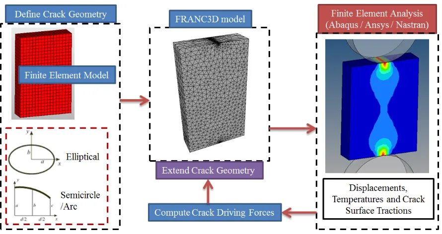
Figure 2.5: Crack growth analysis workflow with FRANC3D [7]

The stress intensity factors (KI, KII and KIII) are of primary importance in the workflow of a

crack growth analysis. In linear elastic fracture mechanics small scale yielding at the crack front is assumed and the stress intensity factor values are governed by,

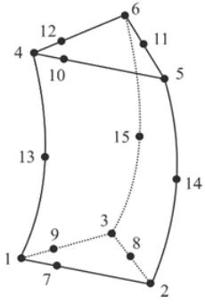
Thus, when performing an analysis of crack growth in a structure characterized by high complexity of geometry and loads, the most critical step is the computation of the stress intensity factors. Figure 2.5 provides a crack growth workflow in FRANC3D program. Crack front elements in FRANC3D are generated with edge quarter point nodes as shown in Figure 2.6. The quadratic Penta element has 15 nodes and quarter points (nodes 7, 9, 10, 12), this configuration allows the element formulation to be altered to capture the singularity due to the crack presence.

Figure 2.6: Crack front element – Penta15 element with quarter points

FRANC3D provides five algorithms for determining the direction of crack growth (kink angle): maximum tensile stress (MTS), maximum shear stress (MSS), maximum generalized stress, maximum strain energy release rate, and planar growth [7], [8].

Crack extensions in different locations on crack front are calculated in FRANC3D based on the equivalent stress intensity factor,

𝐾𝐾𝑥𝑥𝑒𝑒 =�𝐾𝐾𝐼𝐼2+ (𝛼𝛼𝐾𝐾𝐼𝐼𝐼𝐼)2+ (𝛽𝛽𝐾𝐾𝐼𝐼𝐼𝐼𝐼𝐼)2 Eq. (3)

2.3 Fretting Fatigue Crack Growth

Fretting fatigue initiation and damage occurs in contacting components when they are subjected to oscillating normal loads and sliding movements at the same time. At the contact interface surface wear and high contact stress conditions are created under cyclic loading. Fretting is mainly dependent on contact conditions such as surface finish, contact type (edge, spherical, cylindrical, etc.) and coefficient of friction. These factors in turn affect normal force distribution, relative displacement and contact stress magnitudes. The damage obtained due to fretting fatigue can result in fretting wear (permanent material loss), crack nucleation and crack growth leading to catastrophic failure.

and failure may occur in many applications such as bearings shafts, bolted and riveted connections, steel cables, steam and gas turbines.

Figure 2.7 shows a schematic illustration of fretting fatigue. Hojjati et al. [9] performed numerical simulation of fretting fatigue for cylinder on flat and flat on flat models using finite element analysis program ANSYS and fracture mechanics tool FRANC2D/L. The calculation of crack growth cycles was based on Forman NASGRO equation. Hojjati et al observed maximum stress being created in contact regions and stress values were higher near the sharp edge of contact (EOC). The effect of different contact geometries by using different pad sizes on crack propagation behavior were studied [9].

Figure 2.7: Fretting fatigue setup illustration [9]

Dobromirski [10] concluded that the coefficient of friction was the main variable of the fretting process. Mohseni et al. [11] studied the methods used to diminish the effect of fretting on the fatigue life of Al7075-T6 alloy. The effects of various methods including deep rolling, shot peening, laser shock peening, thin film hard coating using physical vapor deposition (PVD), hard anodizing, ion-beam enhanced deposition (IBED), and nitriding to diminish the effect of fretting on the fatigue life were studied [11].

Carter et al. [12] showed crack growth simulation using 3D finite element analysis program (ANSYS) and fracture analysis simulation tool (FRANC3D) in fretting problems at component level [12] wherein static loads were applied at different magnitudes (ramped up or down) to compute total fretting fatigue life (fretting crack nucleation and crack propagation). Barlow et al. [6] calculated stress intensity factors (SIF) for fatigue crack growth simulation in a typical gas turbine engine fan blade attachment using the crack opening displacement approach with FRANC3D and crack propagation trajectories under mode-I and mode-II conditions were obtained using planar, and maximum tangential stress crack-extension criteria.

Prithvi et al. [14] conducted experimental evaluation of fretting fatigue for 7075-T6 aluminum alloys with a test rig mounted on a material test system (MTS 80) to characterize the fretting fatigue damage process and enabled view of the crack initiated in and around the contact zone during the test. The test rig included load cells for normal and friction force measurements. Aditya et al. [15] provided experimental and computational results for fretting fatigue behavior of AISI 4140 vs. Ti-6–4 in a cylinder-on-flat contact configuration. The fretting test fixture was coupled with an MTS machine and gross slip conditions were also considered during fatigue experiments. Aditya et al. [15] used ABAQUS finite element model and considered voronoi tessellation to account for the randomness of the material microstructure and its effects on the fretting fatigue behavior.

Rajasekaran et al. [16] used a coarse finite element model in ABAQUS and developed a semi-analytical model to estimate surface tractions and subsurface stress fields. Fretting fatigue in dovetail blade root of an aircraft gas turbine was simulated using the dovetail approximated as a ‘flat and round’ contact under half-plane assumptions [16]. Rajasekaran et al. applied short crack threshold techniques to predict the effect of friction coefficient on the fatigue behavior of the joint.

load was applied during the test and resulted in the initiation of an initial fretting crack at contact interface, which propagated until final rupture in the middle of the plate.

(a) (b)

Figure 2.8: Fretting test using universal servo-hydraulic fatigue machine [17] (a) Double bolted lap joint specimen (b) Fretting wear obtained in test

Ferjaoui et al. [17] calculated fretting fatigue crack initiation cycles in double lap bolted joint using continuum damage mechanics, wherein finite element analysis program ABAQUS was used to study the effects of different axial stresses and contact forces on fretting relative slip amplitudes and estimate crack initiation lifetime using the process zone approach.

force. A 2D finite element analysis model in ABAQUS was developed and simulated partial and gross slip contact conditions [18]. Jin et al. applied a critical plane based multi-axial fatigue model such as modified shear stress range (MSSR) to characterize fretting fatigue crack initiation behavior.

Figure 2.9: Fretting map [18]

From the different crack growth simulation approaches mentioned in literature, it can be concluded that a more comprehensive analysis of the fretting fatigue phenomena using full vehicle model with highly nonlinear dynamic loads was still missing. The typical simulation process used in the automotive/trucking industries does not identify fretting fatigue and this prevents identifying the root cause for fracture in many cases. Often crack initiation under fretting conditions is mistaken for crack initiation under normal fatigue, this leads to designing an incorrect solution which will add to excessive cost and weight of a vehicle.

2.4 Mixed Mode Crack Growth

Buchholz et al. [21], showed presence of mixed mode effects (Mode II and Mode III) and mode coupling with pure in-plane shear loading of the single edge notched (SEN) specimen having a crack parallel or inclined with respect to the mid-plane between the supports of the specimen. Buchholz [21] performed computational fracture analysis based on the calculation of separated energy release rates (SERRs) with the modified virtual crack closure integral (MVCCI)-method, as implemented in ADAPCRACK3D fracture simulation code.

both drilled holes (r = 2 mm) contain an initial crack (a0 = 5 mm) and are pre-cracked so that

the initial crack forms an angle equal to 45o with respect to the normal to the loading direction.

Figure 2.10: Mixed mode crack growth simulation [20] (a) Plate with two cracks from drilled holes (b) Experimental and simulated crack path

Chao et al. [22] considered the fracture stress in tension “𝜎𝜎_𝑐𝑐” and the fracture stress in shear “𝜏𝜏𝑐𝑐” as two material properties controlling the failure of the material. Chao [22] considered the start of a failure in a solid under a multi-axial stress state by comparing the maximum shear stress and the maximum tensile stress to the strength values of “𝜎𝜎_𝑐𝑐” and “𝜏𝜏_𝑐𝑐” respectively. It was shown as (𝜏𝜏_{𝑥𝑥𝑚𝑚𝑥𝑥}⁄𝜎𝜎_{𝑥𝑥𝑚𝑚𝑥𝑥}) < (𝜏𝜏_𝑐𝑐⁄𝜎𝜎_𝑐𝑐) for a tensile type of fracture and (𝜏𝜏𝑥𝑥𝑚𝑚𝑥𝑥⁄𝜎𝜎𝑥𝑥𝑚𝑚𝑥𝑥) > (𝜏𝜏𝑐𝑐⁄𝜎𝜎𝑐𝑐) for a shear type of fracture [22]. Chao et al. [22] also showed that if

showed that the ratio of fracture stress in tension to shear can be used to characterize the ductility of a mate1ial at the instant of fracture and explain the transition of fracture mechanism for ductile and brittle materials. In Figure 2.11, the critical point is "𝜏𝜏_𝑐𝑐⁄𝜎𝜎_𝑐𝑐 = 0.866” and this predicts tensile fracture to occur for materials with a strength ratio “𝜏𝜏𝑐𝑐⁄𝜎𝜎_𝑐𝑐 > 0.866” and a shear fracture for materials with a strength ratio "𝜏𝜏𝑐𝑐⁄𝜎𝜎_𝑐𝑐 < 0.866” [22].

Figure 2.11: Load mixity (KI/KII) and the material strength ratio 𝜏𝜏𝑐𝑐⁄𝜎𝜎𝑐𝑐 [22]

strain-energy-density factor where the stationary values of this strain-energy-density factor can predict the direction of crack growth under mixed mode conditions. This theory from Sih used the critical value of strain energy density factor as a material parameter for measuring the resistance against fracture and considered it as independent of the crack geometry and loading. Yates et al. [24] discussed stability of crack path under pure and mixed mode loads and the possibility of crack tip plasticity determining direction of fatigue cracks instead of the magnitude of elastic stress field alone. Yates discussed experimental and numerical predicted crack path results and the presence of non-linear strain fields near crack tip, non-uniform and non-proportional loads, crack kinking as the crack grows and evaluating the strength of the mixed mode crack tip stress field. Many other criteria discussed in literature are included in FRANC3D crack growth simulation package to handle mixed mode I/II/III behavior.

included residual stresses in numerical models and used the crack depth function they developed to obtain conservative crack growth life estimates relative to benchmark methods.

Rahman et al. [27] studied fatigue crack growth in compact tension shear specimens under mixed mode loading with effects of overloading on crack growth. Rahman used FRANC2D for stress analysis and for the determination of crack parameters, mixed mode conditions were created by using different loading angles with respect to the normal direction of the crack surface. Rahman et al. discussed the effects of the loading direction, overloading ratio and its load ratio, combination of over-loadings and their locations on the fatigue crack growth and fatigue life. Rahman et al. [28] investigated mixed-mode (I + III) fatigue crack growth of modified compact tension specimen numerically (FRANC3D program) and experimentally to determine the effects of parameters on fatigue life such as crack inclination angle, pre-crack length, crack growth path, fracture surfaces, stress intensity factors along crack front, load ratio and specimen thickness. Rahman observed that the required length for transition from mixed mode to pure mode I conditions increases by increasing the inclination angle and pre-crack length, fatigue life increases by increasing the crack angle and decreasing the pre-crack length and crack front segmentation was observed for all conditions of mixed mode loading.

Figure 2.12. Alegre [29] estimated crack tip stress intensity factors and used maximum principal stress criterion to determine the crack propagation direction.

Figure 2.12: Crack growth simulation with different initial crack angles in a plate subjected to mixed-mode loading [29]

cracks, crack orientation angles, crack growth path and crack propagation life for cruciform aluminum specimen.

Flavien et al. [32] conducted experiments on a cruciform 316L stainless steel specimen with a central hole and an edge crack at the hole using non-proportional loading conditions in order to characterize the load path effect in fatigue crack propagation. Flavien et al. based on their experiments concluded that in non-proportional mixed mode loading conditions, the entire load path should be considered to accurately predict fatigue crack growth and using solely the maximum, minimum and mean values of the stress intensity factors does not provide accurate predictions of the crack growth rate and of the crack path. Flavien observed that crack growth rates and crack path was significantly dependent on the load path applied.

2.5 Crack Growth Simulation Process

crack propagation tool (for example FRANC3D, CRACK3D, ADAPCRACK3D, ZENCRACK, etc.).

Figure 2.13: Typical crack growth simulation process with explicit crack front re-meshing method

definition of contacts between crack faces and the crack front nodes set is defined for extracting displacements, stresses and crack surface tractions. This crack growth model is converted back into finite element format compatible with the analysis solver. The analysis results would then be used with domain independent methods like M-Integral or Interaction integral method to obtain stress intensity factors (KI, KII and KIII values) along the crack front, these computed crack driving forces will then be fed back to the crack propagation tool. The crack growth is determined using appropriate fracture criteria (maximum tensile stress, maximum shear stress, maximum strain energy release rate, etc.) and crack growth rate (paris law, forman equation, NASGRO equation). The crack growth obtained will result in re-meshing of complete model, creation of new crack fronts and definition of new crack face contacts in the model. This model is again converted and analyzed in a finite element program and this process will be repeated until desired length of crack growth or total failure of the model due to critical crack length is obtained.

Spievak et al. [36] proposed using sequence of stress intensity factors from multiple load cases to predict cumulative crack growth direction. In Figure 2.14, it is assumed that the crack grows incrementally during a load cycle and propagation at point “i” only takes place when the change in mode I SIF between load steps is positive, and only when is greater than

the opening SIF at that point [36]. Using simple geometry, the final length, 𝑑𝑑𝑎𝑎𝑖𝑖_𝑇𝑇 , and final angle, 𝜃𝜃_𝑥𝑥𝑖𝑖, after one load cycle are calculated in the following manner,

𝑑𝑑𝑎𝑎𝑇𝑇𝑖𝑖 _{=�(𝑙𝑙}𝑖𝑖₎2_{+ (ℎ}𝑖𝑖₎2 _{Eq. (4)}

𝜃𝜃𝑥𝑥𝑖𝑖 = 𝑡𝑡𝑎𝑎𝑠𝑠−1�ℎ

𝑖𝑖

Figure 2.14: Schematic of crack extension method [36]

The final crack trajectory was approximated by a straight line from the initial crack tip location to the final crack growth location [36].

Carter et al. [12] developed a global/local modeling approach for crack growth simulation where only the region of crack growth influence can be separated from the full model and this reduced local model will have all the crack growth definitions. This sub-model is re-meshed for every crack extension and combined with the rest of the sub-model for analysis. All the boundary conditions on the global/local model are retained and complete load path accounted for crack growth. In Figure 2.15 crack growth simulation model of a turbine disk is shown. A small portion of the disk was extracted for local model and a crack was inserted into the local part. After re-meshing the local model it was then combined with the full model for analysis. The mesh facets and nodes on the cut-surface are retained to maintain compatibility with the full model [12].

2.5.1 Fatigue Crack Growth Rate Model

In the literature many crack growth rate models have been used for different cases, for example, Paris law by Giner et al. [1], Forman–Newman–de Koning (FNK) model by Barlow et al. [6], AFRL crack growth equation by Carter et al. [12], NASGRO crack growth rate equation by Hojjati et al. [9]. A brief description of crack growth rate models are given, a) Paris Law

The Paris growth rate model defines a simple power-law relationship between the crack growth rate and stress intensity factor range. Paris law neglects mean stress effects and is not sensitive to near-threshold or near-critical crack growth behavior. Paris law is given as [1],

𝑑𝑑𝑚𝑚

Where, a is the crack length, N is the number of load cycles, 𝑑𝑑𝑚𝑚

𝑑𝑑𝑑𝑑 provides crack growth rate, C and m are material constants, and ∆𝐾𝐾 is the range of the stress intensity factor, i.e., the difference between the stress intensity factor at maximum and minimum loading.

∆𝐾𝐾 = 𝐾𝐾𝑥𝑥𝑚𝑚𝑥𝑥 − 𝐾𝐾𝑥𝑥𝑖𝑖𝑛𝑛 Eq. (7)

Where, 𝐾𝐾_{𝑥𝑥𝑚𝑚𝑥𝑥} is the maximum stress intensity factor and 𝐾𝐾_{𝑥𝑥𝑖𝑖𝑛𝑛} is the minimum stress intensity factor.

b) Forman equation

Forman equation accelerates crack growth at high R ratios and as KI approaches KIc. 𝑑𝑑𝑚𝑚

𝑑𝑑𝑑𝑑=

𝐶𝐶∆𝐾𝐾𝑚𝑚

(1−𝑅𝑅)𝐾𝐾𝑐𝑐−∆𝐾𝐾=

𝐶𝐶∆𝐾𝐾𝑚𝑚

(1−𝑅𝑅)(𝐾𝐾𝑐𝑐−𝐾𝐾𝑚𝑚𝑚𝑚𝑚𝑚) Eq. (8)

Forman improved the Walker model by describing region III of the fatigue rate curve

and including the stress ratio effect. In the above equation when 𝐾𝐾_{𝑥𝑥𝑚𝑚𝑥𝑥} approaches 𝐾𝐾_𝑐𝑐, 𝑑𝑑𝑚𝑚 𝑑𝑑𝑑𝑑 tends to infinity. This enables Forman equation to represent stable intermediate growth (region II) and the accelerated crack growth rates (region III) [37].

c) NASGRO equation

The NASGROW equation represents the most comprehensive growth law formulation comprising of the mean stress (stress ratio R) effect, threshold, and the true fast fracture and crack closure values [37] [9].

𝑑𝑑𝑚𝑚

𝑑𝑑𝑑𝑑= 𝐶𝐶 �� 1−𝑥𝑥 1−𝑅𝑅��

𝑛𝑛 �1−∆𝐾𝐾𝑡𝑡ℎ_∆𝐾𝐾 �𝑝𝑝

�1−∆𝐾𝐾𝑚𝑚𝑚𝑚𝑚𝑚_{𝐾𝐾𝑐𝑐} �𝑞𝑞 Eq. (9)

𝑓𝑓= 𝐾𝐾𝑜𝑜𝑝𝑝

𝐾𝐾𝑚𝑚𝑚𝑚𝑚𝑚 Eq. (10)

Function “f” accounts for the crack front being open for only a portion of the load cycle due to plasticity induced crack front closure. The value of “f” is related to stress (load) ratio, flow stress and the plane stress/strain constraint factor [9].

2.5.2 Fracture Criteria

The asymptotic stresses for a crack in linear elastic homogeneous materials are given as,

𝜎𝜎𝑟𝑟𝑟𝑟 =_{√2𝜋𝜋𝑟𝑟}1 𝑐𝑐𝑐𝑐𝑠𝑠𝜃𝜃₂�𝐾𝐾𝐼𝐼�1 +𝑠𝑠𝑠𝑠𝑠𝑠2 𝜃𝜃₂�+3₂𝐾𝐾𝐼𝐼𝐼𝐼�𝑠𝑠𝑠𝑠𝑠𝑠𝜃𝜃 −2𝑡𝑡𝑎𝑎𝑠𝑠𝜃𝜃₂�� Eq. (11)

𝜎𝜎𝜃𝜃𝜃𝜃 = _{√2𝜋𝜋𝑟𝑟}1 𝑐𝑐𝑐𝑐𝑠𝑠𝜃𝜃₂�𝐾𝐾𝐼𝐼𝑐𝑐𝑐𝑐𝑠𝑠2 𝜃𝜃₂−3₂𝐾𝐾𝐼𝐼𝐼𝐼𝑠𝑠𝑠𝑠𝑠𝑠𝜃𝜃� Eq. (12)

𝜎𝜎𝑟𝑟𝜃𝜃 = _{2√2𝜋𝜋𝑟𝑟}1 𝑐𝑐𝑐𝑐𝑠𝑠𝜃𝜃₂[𝐾𝐾𝐼𝐼𝑠𝑠𝑠𝑠𝑠𝑠𝜃𝜃+𝐾𝐾𝐼𝐼𝐼𝐼(3𝑐𝑐𝑐𝑐𝑠𝑠𝜃𝜃 −1)] Eq. (13)

Figure 2.16 [7], provides an illustration of kink angle which determines the local direction of crack propagation. The kink angle provides the amount that the crack will deviate from the plane perpendicular to the crack front.

Figure 2.17: Fracture locus using mode I and II stress intensity factors [38]

Figure 2.17, illustrates that crack growth occurs only if the crack driving force is large enough for crack-tip fields to reach the fracture envelope [38]. In Figure 2.17, KI and KII are normalized with respect to KIC.

2.5.2.1 Maximum Tensile Stress Criteria

The MTS theory predicts that a crack will propagate in the direction of maximum "hoop" stress. For materials with isotropic stiffness properties, the hoop stress is related to the resolved mode I stress intensity factor [7],

𝐾𝐾𝐼𝐼(𝜃𝜃) =𝜎𝜎𝜃𝜃𝜃𝜃√2𝜋𝜋𝑟𝑟= 𝑐𝑐𝑐𝑐𝑠𝑠𝜃𝜃₂�𝐾𝐾𝐼𝐼𝑐𝑐𝑐𝑐𝑠𝑠2 𝜃𝜃₂−3₂𝐾𝐾𝐼𝐼𝐼𝐼𝑠𝑠𝑠𝑠𝑠𝑠𝜃𝜃� Eq. (14)

𝜕𝜕𝜎𝜎𝜃𝜃𝜃𝜃 𝜕𝜕𝜃𝜃 = 0,

𝜕𝜕2_𝜎𝜎 𝜃𝜃𝜃𝜃 𝜕𝜕𝜃𝜃2 < 0

The above conditions enable determination of the angle of crack extension “𝜃𝜃”.

𝜃𝜃� =𝑐𝑐𝑐𝑐𝑠𝑠−1_�3𝐾𝐾𝐼𝐼𝐼𝐼2+�𝐾𝐾𝐼𝐼4+8𝐾𝐾𝐼𝐼2𝐾𝐾𝐼𝐼𝐼𝐼2

𝐾𝐾_𝐼𝐼2+9𝐾𝐾_{𝐼𝐼𝐼𝐼}2 � Eq. (15)

where the crack propagation angle 𝜃𝜃� is measured with respect to the crack plane. 𝜃𝜃� = 0 represents crack propagation in a “straight-ahead” direction,

𝜃𝜃� < 0 𝑠𝑠𝑓𝑓 𝐾𝐾𝐼𝐼𝐼𝐼 > 0 𝑎𝑎𝑠𝑠𝑑𝑑 𝜃𝜃� > 0 𝑠𝑠𝑓𝑓 𝐾𝐾𝐼𝐼𝐼𝐼 < 0

2.5.2.2 Maximum Shear Stress Criteria

It is observed that cracks grow in the direction of high shear stress occurs if the crack front experiences high shear loading conditions. The MSS theory predicts that a crack will propagate in the direction of maximum resolved shear stress,

𝜎𝜎𝑠𝑠 = �𝜎𝜎𝑟𝑟𝜃𝜃2 +𝜎𝜎𝑧𝑧𝜃𝜃2 Eq. (16)

For materials with isotropic stiffness properties, the components of the shear stress are related to the resolved mode II and III stress intensity factors [7],

𝐾𝐾𝐼𝐼𝐼𝐼(𝜃𝜃) =𝜎𝜎𝑟𝑟𝜃𝜃√2𝜋𝜋𝑟𝑟 =1₂𝑐𝑐𝑐𝑐𝑠𝑠𝜃𝜃₂[𝐾𝐾𝐼𝐼𝑠𝑠𝑠𝑠𝑠𝑠𝜃𝜃 − 𝐾𝐾𝐼𝐼𝐼𝐼(3𝑐𝑐𝑐𝑐𝑠𝑠𝜃𝜃 −1)] Eq. (17)

2.5.2.3 Maximum Strain Energy Release Rate Criteria

The maximum strain energy release rate criterion states that fracture will occur along the direction where the energy release rate is the maximum and when the energy release rate reaches a critical value [39]. Assuming crack propagates a unit length along its extension, the energy release rate can be given as,

𝐺𝐺 = _𝐸𝐸1′(𝐾𝐾𝐼𝐼2+𝐾𝐾𝐼𝐼𝐼𝐼2) +

1

2𝜇𝜇𝐾𝐾𝐼𝐼𝐼𝐼𝐼𝐼2 , 𝐸𝐸′=�

𝐸𝐸 (𝑃𝑃𝑙𝑙𝑎𝑎𝑠𝑠𝑃𝑃 𝑆𝑆𝑡𝑡𝑟𝑟𝑃𝑃𝑠𝑠𝑠𝑠)

𝐸𝐸_⁄(1− 𝑣𝑣2_{) (𝑃𝑃𝑙𝑙𝑎𝑎𝑠𝑠𝑃𝑃 𝑆𝑆𝑡𝑡𝑟𝑟𝑎𝑎𝑠𝑠𝑠𝑠)} Eq. (19)

The crack initiation angle 𝜃𝜃_𝑜𝑜 is obtained as,

𝜕𝜕𝐺𝐺(𝜃𝜃)⁄𝜕𝜕𝜃𝜃 = 0, 𝜕𝜕2_{𝐺𝐺(𝜃𝜃)⁄𝜕𝜕𝜃𝜃}2 _{< 0 => 𝜃𝜃 = 𝜃𝜃𝑜𝑜}

The crack initiation condition is then given as,

𝐺𝐺(𝜃𝜃𝑜𝑜) =𝐺𝐺𝑐𝑐(𝑥𝑥)

Where 𝐺𝐺𝑐𝑐(𝑥𝑥) is the critical energy release rate function given by [38],

𝐺𝐺𝑐𝑐(𝑥𝑥) = 𝐾𝐾𝐼𝐼𝑐𝑐2(𝑥𝑥)

3.

Chassis Vehicle Dynamics

The Heavy Duty Truck category for class 7 and class 8 vehicles can weigh and transfer up to 80,000 lbf load on road. Trucks move approximately 10 billion tons of freight annually (according to 2014 index), 70% of all freight tonnage moved is on trucks. Any downtime of truck due to structural failure affects the complete supply chain and becomes very expensive for the owner, customer and truck manufacturer.

The chassis of a heavy duty truck is referred to as a frame ladder. It is the backbone of a heavy duty truck and is supported by reinforcement brackets called cross-members along the length of the frame. The frame ladder of a vehicle supports the vehicle cab, powertrain (engine and transmission) components, cooling package (radiator and support brackets), fuel tank and battery system and the payload applied. Figure 3.1 (a) shows that the frame ladder runs along the entire length of a truck and supports all the mounted components. In Figure 3.1 (b) a typical class 8 frame ladder with cross-member arrangement is shown. The location and type of cross-members used depends on the application of the vehicle.

(a) (b)

(a) (b)

Figure 3.2: Frame section (a) Frame web section, lower flange and upper flange (b) Frame sectional property dimensions

The sectional properties of frame rail section (C-Channel) from Figure 3.2 are given as,

Area moment of inertia, 𝐼𝐼𝑦𝑦𝑦𝑦 = 𝐻𝐻3𝑡𝑡 12 +

𝑡𝑡𝑡𝑡 2 �

𝑡𝑡2

3 + (𝑡𝑡+𝐻𝐻)2�, Eq. (21)

Area moment of inertia, 𝐼𝐼_{𝑧𝑧𝑧𝑧}= 𝑡𝑡3𝐻𝐻

12 +𝑡𝑡𝐻𝐻 �𝑌𝑌𝑐𝑐𝑜𝑜𝑐𝑐− 𝑡𝑡 2�

2

+2𝑡𝑡₁₂3𝑡𝑡+ 2𝐵𝐵𝑡𝑡 �𝑌𝑌𝑐𝑐𝑜𝑜𝑐𝑐−𝑡𝑡₂� 2

, Eq. (22)

The Resistance to Bending Moment (RBM) of a frame rail is given as,

𝑅𝑅𝐵𝐵𝑅𝑅= _𝑦𝑦𝐼𝐼𝜎𝜎𝑦𝑦𝑖𝑖𝑥𝑥𝑙𝑙𝑑𝑑 Eq. (23)

Where 𝐼𝐼

𝑦𝑦 is the section modulus of the frame and 𝜎𝜎𝑦𝑦𝑖𝑖𝑥𝑥𝑙𝑙𝑑𝑑 is the yield strength of the frame material which is typically a high strength heat treated steel alloy.

vehicle and cargo. The resistance to bending moment (RBM) value of a frame section is used to select a frame size for a particular application.

3.1 Frame Material Data

The monotonic material properties obtained for a frame section in a typical class 8 heavy duty vehicle ae shown in Table 3.1 below [40].

Table 3.1: Monotonic properties for ASTM A322 Grade 4135[40] Frame Rail Material 0.2% Yield, MPa Ultimate Tensile Strength, MPa Elongation, % Reduction in Area, %

Modulus, GPa Monotonic

Properties 919 952 15 52 199.3

In order to obtain fatigue properties of frame material, six flat tensile specimens were extracted from the frame rail and the specimens were tested at room temperature in accordance with ASTM E8-04 standard [40].

Table3.2: Low cycle fatigue Manson-Coffin model for frame rail material [40] Frame Rail

Material

σf′

E b 𝜀𝜀𝑥𝑥

′ _{c 𝐾𝐾′ 𝑠𝑠′}

Fatigue

Properties 0.00506 -0.051 4.662 -0.992 0.724638 0.017

Table 3.2 above provides strain-life fatigue parameters of a high strength heat treated frame rail material. The Coffin-Manson strain-life model is the sum of two power-fit regression models, the elastic and plastic strain amplitude as a function of reversals to failure,

Δ𝜀𝜀 2 =

σ_f′ E �2𝑁𝑁𝑥𝑥�

𝑏𝑏 +ϵf′

E�2𝑁𝑁𝑥𝑥� 𝑐𝑐

Eq. (24) Where, Δ𝜀𝜀

2 = Total strain amplitude, σ_f′ _{= Fatigue strength coefficient, MPa}

E = Elastic modulus, GPa

b = Fatigue strength exponent ϵ_f′ _{= Fatigue ductility coefficient}

c = Fatigue ductility exponent

Δ𝜎𝜎

2 = 𝐾𝐾′� Δ𝜀𝜀𝑝𝑝

2 � 𝑛𝑛′

Eq. (25) Where, Δ𝜎𝜎

2 = Stress amplitude, 𝐾𝐾′_{= Cyclic strength coefficient, MPa} Δ𝜀𝜀𝑝𝑝

2 = Plastic strain amplitude 𝑠𝑠′ _{= Cyclic strength exponent}

In the below Table 3.3, crack growth results obtained for different open-hole making process using “Metalsa frame rail” [40] are shown,

Table 3.3: Fatigue crack growth results for frame material under different hole making process [40]

Hole Making

Process Paris Values Fracture Properties (MPa √mm) Coefficient “C” Exponent “m” Threshold “Kth” Toughness “KC”

Punch 6e-8 1.82 158.1

2893.5

Drill 2e-8 2.26 177.1

Laser 4e-8 2.23 142.3

Plasma 2e-8 2.23 205.5

hole making process and surface conditioning effect on crack growth parameters. It was observed that frame material has fracture properties with high directional dependency when punching method was used for hole-making process.

Table 3.4: Charpy impact results for heat treated frame rail [40] Frame Rail - Charpy

Impact Results

Energy, ft-lbs

Lateral Expansion (mm)

% Shear Fracture

Room Temperature 40 39 40

-40F 35 40 40

The above Table 3.4 provides Charpy V-notch impact test results for samples extracted from frame rail in the rolled or longitudinal direction. Sean [40] reported that the testing was done in accordance with ASTM E23 standard. Brinell hardness tests were also performed using the fractured tensile specimens according to ASTM E10-07 standard. An average Brinell (BHN) reading of 297 was obtained on the frame rail material [40].

3.2 Finite Element Modelling

analysis. Any local stress concentrations are to be resolved by refining the mesh in the area of interest.

The fasteners (bolts and rivets) used in a vehicle are modeled using “BAR” or “BEAM” one dimensional elements and rigid elements are coupled with these one dimensional elements. The contact definitions between different parts in a full vehicle model are not included. The reason being, a) It does not have large influence on overall dynamic behavior of the frame ladder assembly, b) The computational solution time required for a large full vehicle model with contacts is too expensive to be feasible within design development schedule.

If contact between components are not considered then the load transfer occurs only through bolts and rivets. The inclusion of contact definitions can have large influence on the local stress pattern.

(a) (b)

Figure 3.3: Payload modeling in a full vehicle model (a) Load rack representation (b) Trailer with trailer suspension representation.

beam as non-structural mass on the property card for the beam (CBAR). The mass moment of inertia around the longitudinal axis of the beam in the trailer model is included in a concentrated mass element (CONM2). The trailer suspension is a simplified representation and has only vertical stiffness with damping.

(a) (b)

Figure 3.4: Shocks and suspension modeling in a full vehicle model (a) Shock absorber (b) Rear suspension for a tandem axle

The non-linear force characteristics are considered in NASTRAN using extra point elements (EPOINT). The EPOINT elements are used to represent non-linear damper characteristics, bump stop modelling, leaf spring hysteresis behavior and non-linear tire models. The non-linear forces can be a function of either displacement or velocity.

The axles of a heavy duty truck are modelled using bar elements (CBAR in NASTRAN) and the gears are included as concentrated mass (CONM2 element) at the center of the axle. The axle bump stops are modelled using NASTRAN NOLIN1 card which defines a nonlinear forcing function for transient response analysis.

3.3 Boundary Conditions

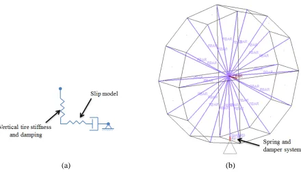
The boundary conditions for dynamic analysis of a full vehicle model are included in the tire model. The tire model generates slip forces in the horizontal plane, and supports the vehicle in the vertical direction through its stiffness. The slip force is nonlinear with respect to both horizontal slip and vertical load.

Figure 3.5: Boundary conditions defined for transient response analysis of a full vehicle model

In Figure 3.6 (a) simplified representation of tire is done using a spring-damper system. The damping of tire is relatively small, about 0.1% of the tire stiffness. The simplified tire models will have a one-point contact with the road and the enveloping effect of tire is calculated using the effective road surface as an input for the tires instead of the physical road profile.

Figure 3.6 (b) shows a complete tire model used for full vehicle model, where the tire stiffness is defined at the bottom tire-ground interface and boundary conditions are specified at the lower end of the spring model.

The viscous damping specified for shock absorbers and rubber bushings are defined by structural elements, such as, NASTRAN CDAMP1 entry as well as by using direct matrix input (DMIG). Structural damping is also entered on the NASTRAN material definitions (PARAM G input).

(a) (b)

Figure 3.6: Simplified tire model (a) Tire model representation with spring-damper system (b) Full tire model with tire stiffness defined at tire-ground interface

3.4 Endurance Testing of Vehicles

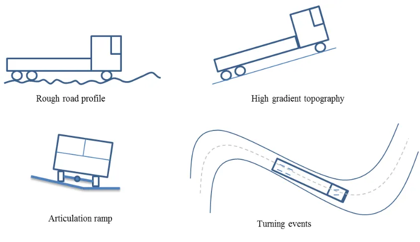
frequency sweeps, quasi-static articulation and axle roll events, low and high speed maneuvering (turning) events, braking and high gradient topographical events. Accelerated endurance test of a complete vehicle provides,

a) Correlation between known field issues and proving ground failures b) Good knowledge of new product durability before customer usage c) Reduced test time and cost of product development

d) Identifies components that are sensitive to vibrations at certain frequencies, others that are sensitive to lateral forces, torsion and certain test maneuvers.

Depending on the operational class to which the vehicle is used different testing events are selected. Figure 3.7 provides schematic representation for some of the endurance test events used for full vehicle validation,

Endurance testing is done at different speeds and at different gross vehicle weight rating (GVWR). These test events provide dynamic interactions between different vehicle modules and sub-systems, enables dynamic interference and clearance check. The test vehicle will be instrumented with strain gages, load transducers and accelerometers to measure vehicle response during testing. The data measured (strain, displacement and acceleration history) are used to validate new designs and improve numerical model development. The number of repeats for each event was defined depending on the operating class to which the vehicles are targeted. The damage obtained during test will be scaled for repeated cycles to estimate cycles to failure. The accelerated damages and wear obtained on different vehicle parts are then inspected and studied to follow up with design modifications.

Figure 3.8: Vehicle data acquisition from endurance test

will identify the structural performance and dynamic behavior. Frequency response of measured data will be compared with modal results obtained in simulation to determine the eigen-vectors. Power spectral density (PSD) plots provide the frequency response of a random or periodic signal and identifies where the average power is distributed as a function of frequency. A PSD plot identifies the high and low energy content of a vehicle response along frequency distribution. Level crossing analysis counts the number of times the signal crosses a number of specified levels with positive slopes above zero and negative slopes below zero.

3.5 Simulation Process

In Figure 3.9, the simulation process typically used for root cause investigation using full vehicle durability analysis is shown. In this process the finite element representation of a full vehicle model was a structured assembly of different components in a heavy duty truck. This vehicle model was mainly represented to capture the stiffness of different components with a relatively coarse mesh. The brackets and plates used for most part of the vehicle were represented using Shell elements (CTRIA3 and CQUAD4 elements in NASTRAN), castings and extruded sections represented using Solid elements (CTETRA10 and CHEXA8 elements in NASTRAN). The model includes one dimensional multi point constraints to represent connections using bolts, rivets and springs (RBE, CBAR, CBEAM and CELAS elements in NASTRAN).

The shock absorbers and isolators of the vehicle are represented in the model with dampers (CDAMP and CBUSH elements in NASTRAN). This model will have boundary conditions defining load application at tire patches and mass distribution at its center of gravity (e.g., trailer, fuel tank, battery box, cab and other suspended elements from a truck). The modal damping used was 3% of critical damping for the entire frequency range. The transient loads used represent the digital representation of track surface (proving grounds). The response obtained from analysis (forces, accelerations and stress) represent vehicle response to proving ground inputs. This model demands computationally large storage and solution time.

component level model (for example the component level model can be a small bracket bolted in a large assembly and interface loads are obtained through the assembled joints of the bracket). The component level model was then solved for a set of static unit load cases representing the applied forces acting on it. The force histories were calculated from transient analysis of full vehicle model and the stress in an element was calculated as a summation of the unit load case stresses multiplied by the force histories (linear superposition),

σx(t) =�n_i=1Sx,i. Fi(t) Eq. (26)

where n is the number of unit load cases representing the number of interface nodes.

The stress history was then used with appropriate material stress-life (S-N) curve to determine the number of fatigue cycles to failure. This fatigue analysis can then determine the damage per event among multiple test events and identify the total damage for the complete endurance test. The objective of a root cause investigation is to identify,

a) The event with maximum damage for subsystem model,

b) Area of high stress on component level model correlating with physical failure location,

c) Cycles to failure in simulation correlating with physical test report.