DEVELOPMENT OF HAZARD CONSISTENT SEISMIC FRAGILITY
CURVES BY NUMERICAL ANALYSIS - APPLICATION TO SMART2013
Irmela Zentner1, Nicolas Bonfils2
1
Research Engineer, EDF R&D Clamart, France
2
Engineer, EDF SEPTEN Villeurbanne, France
ABSTRACT
The Probabilistic Risk Assessment (PRA) methodology is used worldwide to assess the seismic safety of nuclear power plants. Concurrently, in civil engineering, the performance based earthquake engineering (PBEE) methodology is becoming the state of the art for design and verification of engineered structures whose seismic performance has to meet safety and economic needs. In this context, the structural reliability is generally characterized by fragility curves, expressing the failure probability of the structure or component as a function of seismic ground motion intensity (for example peak ground acceleration or spectral acceleration). In general, a lognormal model is assumed. Moreover, in the recent years, nonlinear transient analyses have become the preferred approach for the evaluation of seismic performance of buildings. Such analyses rely on structural models and the explicit propagation of uncertainty and variability due to random excitation. This paper presents a new methodology for the numerical evaluation of fragility curves from a reduced set of site specific scenario earthquakes. The evaluation of the fragility curves is based on a general bivariate probability model and does not require scaling of the accelerograms. It allows for probability distributions other than lognormal. The proposed methodology is applied to a reinforced concrete building studied during the SMART2013 benchmark project and the results are compared to lognormal fragility curves obtained by regression.
INTRODUCTION
A fragility curve is a function that expresses the probability of failure of a structure or component as a function of the intensity of external aggression. In the recent years, various methods to determine fragility curves have been proposed in the literature. The increased interest is, among others, motivated by the ongoing implementation of performance based earthquake engineering (PBEE) procedures in civil engineering design. In the US, the Applied Technology Council (ATC) implemented the PBEE methodology to be used for civil structures. A comprehensive set of procedures to estimate fragility functions from data is proposed in ATC-58 and Porter et al 2007. In particular, the fragility analysis methods have to depend on the nature and number of available data. In the nuclear sector, the seismic Probabilistic Risk Assessment (PRA) dates back to the 70ies and is now widely used for the evaluation of plant safety, e.g. EPRI 2003. Still today, the analysis methods of seismic PRA are based on the pioneering work of Kennedy in the early 80ies.
COMPUTATION OF FRAGILITY CURVES
Literature review
The fragility function expresses the conditional probability that the structure fails or reaches a certain damage state, given the intensity of aggression a. The intensity of the aggression is characterized by the so-called earthquake intensity measures (IM). The most popular IM for the evaluation of fragility functions are the peak ground acceleration PGA and pseudo-spectral acceleration PSA at a fundamental frequency of the structure. The methodologies are not limited to this case but hazard curves are generally available for these two IM. The structural damage or failure is characterized by a Damage Measure DM denoted here Y. The latter can be a continuous variable such as the interstorey drift or discrete indicating the membership to a certain damage state or failure. In the first case, the fragility curve yields:
)
(
)
(
a
=
P
Y
>
DC
IM
=
a
P
f . In the latter case, the DM is a binary variable taking value 1 if failureoccurs and 0 otherwise, such that
P
f(
a
)
=
P
(
Y
=
1
IM
=
a
)
. Obviously, the choice of the method used for the evaluation of fragility curves has to be in agreement with the type and number of data available. This is explained with more detail below. In practice, the structural capacity is generally assumed to be lognormally distributed which yields the lognormal fragility curve:÷÷
ø
ö
çç
è
æ
-F
=
b
a
a
mf
A
P
(
)
ln
ln
(1)Where Am is the median capacity of the structure or component and b is the lognormal standard deviation. In nuclear industry practice, the Safety Factor method is generally used to determine the parameters of the lognormal fragility curve (1). It is based on the evaluation of margins, related to the different modelling assumptions, and with respect to the design analysis. In particular, the median capacity is obtained as the product of the different best-estimate margins and the design basis earthquake. The method can be carried out with analytical calculations and does not need time-consuming numerical simulations. On the other hand, fragility curves can be determined by means of numerical simulation when a structural best-estimate model is available. In this framework, the seismic excitation is then represented by a set of time histories. Classical statistical methods for the evaluation of fragility curves, when input - output samples are available, are:
· Method of moments e.g. Reed & Kennedy 1994, Porter et al 2007. It can be used when a sample of capacities has been observed: this is the case in incremental dynamic analysis or when qualification tests until failure are available.
· Maximum likelihood method, e.g Zentner et al 2011. This method requires demand data before and beyond failure and a discrete damage measure. It is the most adequate in the case of discrete (binary) data such as buckling as failure criterion.
· Fitting of a linear seismic demand model in the log-scale by means of linear regression, e.g. Ellingwood & Kinali 2009, Zentner et al. 2011. This method is applicable for any kind of data but it means extrapolation of the behavior beyond yield if no failure is observed.
overcome model assumptions such as lognormal probability distribution but this is at the expense of more data for the same precision.
Linear regression approach
The method assumes that a sample of N input-output pairs, (ai, yi), i = 1,...N, is available. The input is the ground motion indicator (seismic intensity level ai) and the output variable yi is the continuous damage measure. The continuous damage measure Y is modelled as lognormal random variable:
h
a
cb
Y = (2)
where h is a lognormal random variable with a median of 1 and a logarithmic standard deviation s . It is supposed that the structure fails or reaches a certain damage level when the variable Y exceeds a threshold
DS such that Pf(a) = P(Y > DS|a)
.
The parameters b, c and scan be conveniently determined by linear regression: ε, + ) ( c + b =(Y) ln( ) ln a s
ln (3)
where se = log(h) is a centred normal random variable with std s, the latter is obtained as the standard deviation (std) of the regression error. Moreover, defining DS= b∙Amc we have
úû ù êë é c (DS/b) =
Am exp ln . (4)
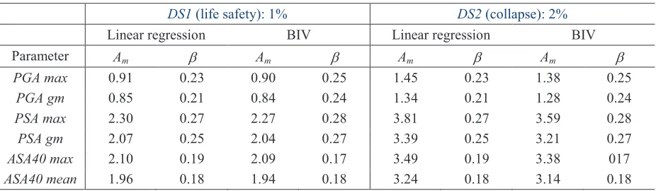
In consequence, the fragility curve is described by a lognormal distribution with a median equal to the seismic capacity Am and the lognormal standard deviation b = s/c. One major advantage of the linear regression approach is that it can be used even in cases when no failure is observed. It does not require scaling of accelerograms and is quite robust even for small sample sizes. In the linear regression approach, the b-value does not depend on the failure threshold (cf Table 1). The increasing dispersion with increased DM is however accounted for by assuming a lognormal model (the std increases with increasing DM). This is known as heteroscedastic behaviour in the statistics community.
GENERAL BIVARIATE FRAGILITY MODEL
Methodology
If the joint distribution of intensity and damage measures is known, then it is possible to evaluate the conditional probability distribution using the Bayes theorem. This is the idea of the approach presented in this section. We consider the two random variables IM, Y defined respectively as the ground motion intensity and the damage measure together with their joint distribution f(y,im). Then, the conditional probability of y knowing IM=a is
)
(
)
,
(
)
(
a
a
a
f
y
f
IM
y
f
=
=
(5)and we can evaluate the fragility function for any given damage level threshold DS as:
ò
¥ = = > = DSf f y dy
f IM
DS Y P
P ( , )
) ( 1 ) ( ) (
a
a
a
a
(6)case, the lognormal distribution of the IM is known a priori and completely determined by the GMPE. Here, we will focus on Gaussian copula. That is a standard Gaussian correlation model characterized by a correlation coefficient r associated to the two variables IM and Y with marginal Cumulative Density Functions (CDF) ܨܫܯ and ܨܻ. The Gaussian copula model yields the following expression for the joint distribution of the intensity and the damage measure:
(
(
),
(
)
)
(
(
(
)),
(
(
))
)
)
,
(
2 1 11 1 1 2
1
u
u
u
F
F
y
u
C
rN=
F
rF
-F
-=
F
rF
- IMa
F
- Y, (7)
where u1 and u2 are standard uniform random variables. For discrete damage states or structural failure,
binomial or multinomial distributions are adequate probability distributions. Candidate distributions for continuous damage measures are for example the lognormal distributions and the family of extreme value distributions. The unknown model parameters have to be inferred from data as described in the next section.
Model identification and selection
The set of parameters related to the bivariate fragility model, denoted by qM, comprises the two
parameters of the lognormal intensity measure, the correlation coefficient and the parameters of the damage measure. In order to select the most plausible model M and its parameter values ߠܯ given the data we can use classical information theory. This can be achieved by using the maximum likelihood estimator (MLE). Using again the Bayes theorem, the likelihood function for this problem reads:
Õ
Õ
= -= i i i i i M i i MM f y f y f
L M 1 ) ( ) , ( ) , ( )
(
q
a
q
qa
a
(8)The most plausible set of parameter values is obtained by minimizing the negative log-likelihood: )
( ln min arg
ˆM LM
q
Mq
= - . Moreover, the most plausible model M is the one with the highest likelihood score. Often, the Bayesian Information Criterion (BIC) is used:p S M
M
N
N
L
BIC
=
-
2
ln
(
q
ˆ
)
+
ln(
)
(9)It depends on the likelihood function LM, the number of model parameters Np and the sample size Ns and
gives a preference to the simpler model, featuring less parameters, in order to avoid over-fitting. This is however not an issue here, since only standard probability distributions, featuring a small number of parameters (2-3) are used.
Bivariate lognormal model
The bivariate lognormal model allows to express the fragility curve as
÷ ÷ ø ö ç ç è æ -F = Y f DS m P ln 2 1 ) ln( ) ( ) (
s
r
a
a
(10)where ݉ሺߙሻൌߤߤ݈ܻ݊ ߪ݈ܻ݊Ȁߪ݈݊ܫܯߩሺ݈݊ߙ െ ߤ݈݊ܫܯሻ.
generally not the same as the unconditional distribution (y). This problem can be tackled by using the conditional MLE of equation (8).
Other interesting features
The bivariate fragility model proposed here does not dependent on the choice of the particular distribution of the IM, as highlighted by equation (8). This results from the mathematical definition as a conditional probability, given the IM. The fragility curves are however site-specific as they do depend on the particular spectral shape and other features linked to the scenario (such as duration and other IM) through the set of accelerograms used for the structural analysis.
The uncertainty related to the intensity measures is a particular issue when empirical fragility data is used. In particular, when the epistemic uncertainty related to the IM is accounted for in the hazard curve, it should not be included in the fragility in order not to double count that uncertainty. However, when dealing with numerical fragility curves that are based on time history analysis, then this is not the case because of the proper definition of the fragility curve: it expresses a conditional probability, i.e. the failure probability given a particular value of ground motion intensity measure.
Another interesting feature of the numerical approach presented in this paper is the possibility to directly introduce the known distribution of the IM. As for the linear regression approach, there is no need for scaling of accelerograms or binning.
GROUND MOTION TIME HISTORIES
The ground motion time histories used for the evaluation of fragility curves constitute the link between the seismic hazard and the fragility analyses. Ideally, the seismic load should be hazard consistent, site specific and comply with design spectra.Moreover, more recent guidelines such as ATC-58 do require realistic description of seismic load for performance based safety assessment methods.
In the framework of performance based analyses, the simulated or selected ground motion has to have realistic spectral shape. Other ground motion intensity parameters have to be computed and compared to the databases and predicted values, given the scenario(s). For this purpose, both median and standard deviation (or ±1s values) of the ground motion parameters have to be evaluated. In general, the seismic load to be considered for design and verification is defined by pseudo-spectral accelerations (PSA) provided by the target response spectra.
The methodology used for the simulation or selection of ground motion has to be in agreement with the scope and the type of target spectrum, scenario or design:
· One or more target scenarios: ground motion time histories match distribution of target spectra (median and std)
· Uniform Hazard Spectrum UHS: disaggregation allows to define a collection of conditional spectra related to different scenarios, ground motion matches the conditional spectra (Lin et al 2013).
then it is generally necessary to select ground motion from different magnitudes, distances and sites in order to obtain a set that is in agreement with the target spectra.
APPLICATION TO SMART BENCHMARK REINFORCED CONCRETE BUILDING
Structural best-estimate model
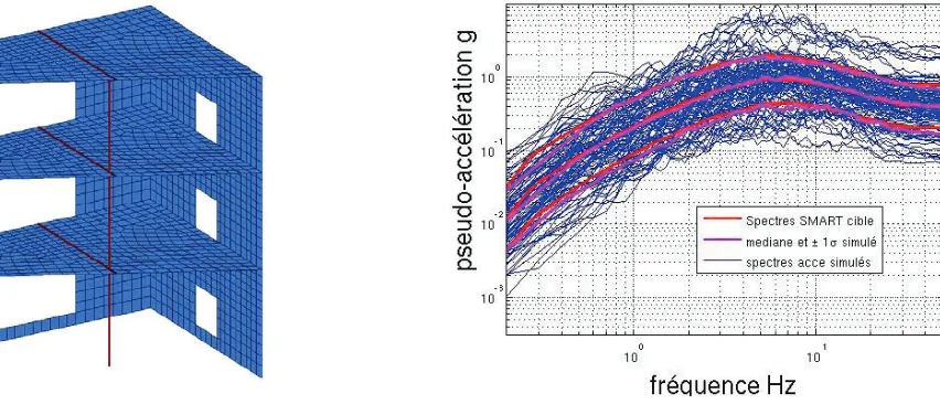
This structure has been the object of numerous experimental and numerical studies in the framework of the SMART2008 and more recently the SMART2013 benchmark contest. The finite element model, shown in Figure 1, contains shell and beam elements. The model constructed for the 2013 benchmark includes the shaking table since interaction was found to be important. For the computation of the fragility curves, the support of the mock-up, that is the shaking table, was modelled by equivalent springs. The properties of these springs were provided by the benchmark specifications. More information can be found on the dedicated website: http://smart2013.eu. The numerical transient analyses are performed with the opensource multipurpose FE software Code_Aster (\http://www.code-aster.org). Nonlinear structural behaviour is accounted for by the homogenized nonlinear constitutive model for reinforced concrete GLRC_DM available with Code_Aster and Rayleigh damping is assumed.
Figure 1. SMART benchmark model (left) and response spectra of simulated accelerograms together with the target in red (right).
Seismic input
The ground motion time histories are artificial accelerograms obtained with a stochastic ground motion model implemented in Code_Aster. A set of 50 couples of horizontal ground motion (XY) was simulated to match the scenario target spectrum in median and ±1s values. The target spectra (red curves) are shown on Figure 1 together with the respective values of the simulated accelerograms (magenta curves). The target spectrum is a conservative design spectrum associated to a magnitude M=6.5 and distance D=9 km event for a rock site (according to French regulation RFS-2001-01). It has been checked that median and log-std of other indicators (PGA, PGV, CAV) are in agreement with the site-specific hazard.
The intensity measures IM considered here are Pseudo-Spectral Acceleration at the first fundamental frequency of the structure (PSA), Peak Ground Acceleration (PGA) and Average Spectral Acceleration ASAR (De Biasio et al 2014). The latter indicator is obtained by integration of the PSA values in a defined frequency range (here R=40%) in order to account for structural damage leading to a decrease of the fundamental frequencies of the structure. For PGA and PSA, both the geometrical mean (gm) and the maximum value of the two horizontal directions is considered. For the ASA, the mean and the maximum are considered. The IMs are assumed to have a lognormal marginal distribution, as predicted by the GMPE.
Evaluation of fragility curves
In this section, fragility curves are evaluated by linear regression and using the more general bivariate probability model. The structure is submitted to the 50 pairs of horizontal time histories described above. These are the accelerograms that were provided for the SMART2013 benchmark. In order to obtain ground motion time histories that are more likely to damage the structure, these time histories were multiplied by a factor 2 even though the use of conditional spectra would be more rigorous. The IM is assumed lognormal, according to seismological models and in agreement with the the ground motion simulation procedure. The adequateness of Lognormal (LN), Weibull and Generalized Extreme Value (GEV) distributions to represent damage measures is analyzed. By the extreme value theorem, the GEV distribution is the only possible limit distribution of properly normalized maxima of a sequence of independent and identically distributed random variables. The generalized extreme value distribution (see Coles, 2001) has 3 parameters, namely the shape, scale and location parameters. The shape parameter determines the type of GEV (type I, II, III), where type I is the Gumbel distribution, type II is the Fréchet distribution and type III is the reversed Weibull distribution (distribution of minima). The dependency is modeled by a Gaussian copula, characterized by the rank correlation coefficient r between intensity and damage. The statistical analyses are performed with Matlab and the Statistics toolbox.
Table 1: Fragility curve parameters obtained with linear regression and the bivariate fragility model, median capacities are expressed in (g).
DS1 (life safety): 1% DS2 (collapse): 2%
Linear regression BIV Linear regression BIV
Parameter Am b Am b Am b Am b
PGA max 0.91 0.23 0.90 0.25 1.45 0.23 1.38 0.25
PGA gm 0.85 0.21 0.84 0.24 1.34 0.21 1.28 0.24
PSA max 2.30 0.27 2.27 0.28 3.81 0.27 3.59 0.28
PSA gm 2.07 0.25 2.04 0.27 3.39 0.25 3.21 0.27
ASA40 max 2.10 0.19 2.09 0.17 3.49 0.19 3.38 017
Figure 2. Fragility curves for PSAgm and ASA40mean with threshold DS1.
Figure 3. Example of scatter plots and fragility curves for PSAgm with DS2.
The resulting fragility curves are shown in figure 2 and figures 3 and 4, on the right side, for two intensity measures: the geometric mean PSA and the mean ASA40. Both indicators are evaluated for the first fundamental eigenfrequency of the structure. Figure 2 shows the fragility curve for the life safety damage threshold DS1 while the figure 3 and figure 4 show results for the collapse threshold DS2. The bivariate fragility model also allows to simulate more input-output data. This is illustrated in the figures 2-4 on the left where the scatter plots for the date (red) and the bivariate Weibull (green), GEV (magenta) and lognormal (blue) models are shown.
Table 1 shows the parameters of the fragility curve obtained by regression and compares them to the lognormal bivariate model where the MLE accounting for the conditional DM sample is used.
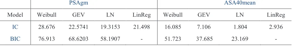
for the linear regression model and shown in table 2. As expected, the lognormal bivariate model is more plausible than the regression model, given the data.
Obviously, the epistemic uncertainty was not fully accounted for in the numerical simulation. The respective bU value has to be added to the results of the numerical analysis.
Figure 4. Example of scatter plots and fragility curves for ASA40mean with DS2.
Table 2: BIC and IC evaluated for different indicators with bivariate fragility model and the linear regression parameters (LinReg)
PSAgm ASA40mean
Model Weibull GEV LN LinReg Weibull GEV LN LinReg
IC 28.676 22.5741 19.3153 21.498 16.085 7.106 1.804 2.936
BIC 76.913 68.6203 58.1907 - 51.723 37.685 23.169 -
SUMMARY AND CONCLUSION
reinforced concrete structure (SMART2013 model) shows that the results for lognormal and GV are quite close, there is more discrepancy for higher damage thresholds. For this application the most plausible model is the bivariate lognormal distribution.
T
he epistemic uncertainty is often not fully be accounted for in the numerical simulation. In this case (as here), the respective bU value has to be added to the results of the numerical analysis.In order to optimize and possibly reduce the number of structural analysis to be performed, more advanced design of experiments could be used, in particular for the selection of accelerograms. The preferred sampling in the regions of interest, close to structural capacity, will be investigated in further studies.
REFERENCES
Baker, J. (2015). Efficient analytical fragility function fitting using dynamic structural data. Earthquake Spectra, in press.
Code_Aster, Multi-purpose FEM Code, R4.05.05 Génération de signaux sismiques and U2.08.05 Propagation des incertitudes et calcul de courbes de fragilité. http://www.code-aster.org
Coles (2001), An introduction to statistical modelling of extreme values. Springer Series in Statistics. De Biasio, M., Grange S., Dufour F., Allain, F. and Petre-Lazar I., (2014). A Simple and Efficient
Intensity Measure to Account for Nonlinear Structural Behavior. Earthquake Spectra 30(4), 1403-1426.
Ellingwood, B. and Kinali, K. (2009) Quantifying and communicating uncertainty in seismic risk assessment. Structural Safety 31(2).
Haselton, et al. (2014). Response-History Analysis for the Design of New Buildings: A Fully Revised Chapter 16 Methodology Proposed for the 2015 NEHRP Provisions and the ASCE/SEI 7-16 Standard. U.S. National Conf. on Earth. Engrg, Anchorage, Alaska.
Jayaram, N., Lin, T., and Baker, J. W. (2011) A computationally efficient ground-motion selection algorithm for matching a target response spectrum mean and variance. Earthquake Spectra, 27(3), 797-815.
Liel, A., Haselton, C., Deierlein G. and Baker J. (2009). Incorporating Modeling Uncertainties in the Assessment of Seismic Collapse Risk of Buildings, Structural Safety, 31.
Lin T., Haselton C., Baker J., (2013) Conditional spectrum-based ground motion selection. Part I and II. Earthquake Engng. Struct. Dyn.
Noh, Lallemand, Kiremidjian (2014), Development of empirical and analytical fragility functions using kernel smoothing methods Earthquake Engrg and Struct. Dynamics 10(1).
Porter, K., Kennedy, R. and Bachman, R. (2007). Creating Fragility Functions for Performance-Based Earthquake Engineering. Earthquake Spectra 23(2), 471-489.
Reed J.W., Kennedy R.P. (1994). Methodology for Developing Seismic Fragilities. Final Report TR-103959, EPRI.
Richard, Benjamin and Chaudat, Thierry. (2014). Presentation of the SMART2013 International Benchmark. 2014. SEMT/EMSI/ST/12-017 H.
Zentner, I., Humbert, N., Ravet, S. and Viallet, E. (2011). Numerical methods for seismic fragility analysis of structures and components in nuclear industry - Application to a reactor coolant system.
Georisk 2(5), 99-109.
Zentner, I. (2014). A procedure for simulating synthetic accelerograms compatible with correlated and conditional probabilistic response spectra. Soil Dyn Earth Eng. 63(1), 226-233.