Rmind: a tool for cryptographically secure
statistical analysis
Dan Bogdanov1, Liina Kamm1,2, Sven Laur2 and Ville Sokk1
1
Cybernetica, Tartu, Estonia {dan, liina, ville.sokk}@cyber.ee
2University of Tartu, Institute of Computer Science, Tartu, Estonia [email protected]
Abstract. Secure multi-party computation platforms are becoming more and more practical. This has paved the way for privacy-preserving sta-tistical analysis using secure multi-party computation. Simple stasta-tistical analysis functions have been emerging here and there in literature, but no comprehensive system has been compiled. We describe and implement the most used statistical analysis functions in the privacy-preserving set-ting including simple statistics, t-test,χ2test, Wilcoxon tests and linear regression. We give descriptions of the privacy-preserving algorithms and benchmark results that show the feasibility of our solution.
Keywords: Privacy, statistical analysis, hypothesis testing, predictive mod-elling, cryptography
1
Introduction
Digital databases exist wherever modern computing technology is used. These databases often contain private data, e.g., the behaviour of customers or citizens. Today’s data analysis technologies require that the analysts have direct access to the data, thus creating a risk to privacy. Even if data analysts are diligent and keep secrets, the data in their possession can leak through an external attack.
Cryptographic research has given us encryption schemes that protect databases until the data are processed. However, existing analysis tools require us to de-crypt data before processing, bringing us back to the privacy problem. Emerging cryptographic technologies like secure multi-party computation (SMC) solve the problem by allowing data to be processed in encrypted form. This enables a new kind of computer that can manipulate individual data records without seeing them—much like a blind craftsman sculpting a work of art.
Secure multi-party computation was considered impractical for years, but clever protocol design and determined engineering have led to first real-world applications [12, 11]. Therefore, we decided to investigate the feasibility of using SMC to perform statistical analyses with better privacy.
First, statisticians were used to seeing individual values and were unsure if they can find inconsistencies and ensure analytical quality without such access. SMC takes away control from the analyst by only disclosing the query results.
The second concern was the lack of user-friendly tools for cryptographically secure data analysis. Statisticians are used to the workflows of interactive en-vironments like SAS, SPSS and R. The interviewees expected to see a drop-in replacement of their environment with the new privacy guarantees.
In this paper, we describe a suite of preserving algorithms for privacy-preserving filtering, descriptive statistics, outlier detection, statistical testing and modelling. We implement these algorithms inRmind, a cryptographically secure statistical analysis tool designed to provide a similar experience to existing script-able tools such as R1.Rmind provides tools to support all stages of statistical analysis—data collection, exploration, preparation and analysis.
In 2014, we presented the Estonian Data Protection Agency with a proposal for linking and analyzing two government databases using the tools and methods presented in this paper. Their conclusion was that, according to the legislation, our method does not process personally identifiable information and thus no permit is needed as long as our technical solution is used and the study plan is followed [5]. While this is not yet the prevailing legal position, it marks a paradigm shift in data protection.
Our contribution.This paper builds on our earlier work in [5, 37] where we pre-sented our first attempts on privacy-preserving statistics. In this paper, we have made major improvements. First, we designed and implemented new privacy-preserving algorithms for statistical testing including popular value correction methods for multiple testing. Second, we designed and implemented privacy-preserving methods for multivariate linear regression, which can be easily ex-tended to polynomial regression or linear regression with regard to other basic functions. For this, we developed privacy-preserving methods for solving a set of linear equations based on Gaussian elimination with backsubstitution and LU decomposition. Both are, of course, applicable in other contexts beside statis-tics. The same applies to our novel privacy-preserving version of the conjugate gradient method for minimizing quadratic forms.
Third, we presentRmind, a privacy-preserving statistical analysis environ-ment designed to resolve user acceptance issues. Rmind supports a complete data analysis process where data are collected from various sources, linked and statistically analysed. The user interface is identical to that of R. We also took great care to fix all details of our algorithms so that they provide the same results as the R tool, to the precision of a floating point comparison.
Fourth, we have implemented the new algorithms, optimised the previous implementations, and provide new performance results that prove the feasibility of the system. Comparable performance results for the entire suite of statistical operations have not been published and thus it has been difficult to estimate whether cryptographically secure statistical analysis is practically feasible or not.
1
Related work.The closest system to what we propose has been introduced by Chida et al. in [19]. They are using the statistics environment R to create a user interface to a secure multi-party computation backend. They have implemented descriptive statistics, filtering, cross-tabulation and a version of the t-test and
χ2 test. Their protocols combine public and private calculations and provide impressive performance. However, their implementation is limited in the kinds of analyses they can perform due to their lack of support for real numbers. Their implementation also does not support linking different database tables.
Another recent implementation with similar goals is by El Emam et al [25]. They provide protocols for only linking and the computation of χ2 tests, odds ratio and relative risk. Other published results have focused on individual com-ponents in our statistics suite, e.g, mean, variance, frequency analysis and re-gression [16, 21, 22, 41, 40], filtered sums, weighted sums and scalar products [53, 56, 36]. Related papers on private data aggregation have also targeted stream-ing data [50, 45]. However, all of these components have been implemented as separate special purpose programs using various programming languages and dif-ferent underlying secure multi-party computation protocol sets. It would be very difficult, if not impossible, to integrate these programs into one comprehensive statistics suite.
2
Designing a tool for secure statistical analysis
2.1 Requirements for a secure statistical analysis tool
There is a perceived need of cryptographic security capability in the following privacy-preserving data integration scenario [5].
1. Data owners and analysts agree on the data format and the study plan. 2. Data owners upload their inputs to a secured database.
3. Data analysts send queries that are in the study plan.
4. Analysts receive analysis results and interpret them in a resulting report.
We propose a tool for performing privacy-preserving statistical studies in the given setting using secure multi-party computation. The difference between
Rmindand standard statistical tools is thatRmindcollects and analyses data in encrypted form without decrypting them and gives provable privacy guarantees to the analysis process. This efficiently ensures that the data owner is the only party with access to the private inputs and only the results of the analysis are disclosed to the analyst.Rmindis designed with the following goals:
1. Similarity to existing tools.Based on the interviews, the end users prefer tools with familiar user interfaces.
2. Separation of public and private data.The tool should separate public and private values in data.
4. Features chosen according to real-world needs.Data transformation and analysis features are chosen after interviews with statisticians to deter-mine the tools they most commonly use.
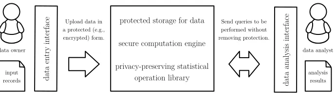
protected storage for data
secure computation engine
privacy-preserving statistical operation library
Upload data in a protected (e.g., encrypted) form.
input records data en
try in
terface
data analysis in
terface
Send queries to be performed without removing protection.
data owner data analyst
analysis results
Fig. 1.Design of a privacy-preserving statistical analysis tool and interfaces based on secure computation
The main components ofRmindare the data entry interface, the data analy-sis interface and the storage and computation backend (see Figure 1). Standalone data entry or analysis interfaces can be implemented on any programming plat-form supported by the secure multi-party computation framework. Data are tagged public or private during the upload to allow the statistical tool to apply secure multi-party computation on private data. As the study plan is public, we do not need to hide data formats or the algorithms being executed. However, private parameters to the queries can be hidden from the computing parties as any other private inputs, e.g., the criteria for forming subgroups can be kept secret.
2.2 Secure multi-party computation with external parties
Secure multi-party computation (SMC) is a cryptographic technology for com-puting a function with multiple parties where only the party who provided a par-ticular input can see that input and every party only gets the output specifically intended for them. In the standard model, partiesP1, . . . ,Pn jointly evaluate a functionf(x1, . . . , xn) with outputs (y1, . . . , yn) so thatPi submits its inputxi and learns the outputyi and nothing about the other inputs and outputs.
Not all parties in the data integration scenario have the resources and moti-vation to participate equally in the secure analysis. Therefore, we consider three different party types.Input parties(data owners) provide the inputs to the anal-ysis and expect that nobody else learns them. Computing parties store inputs, participate in secure multi-party computation protocols and give outputs to the
result parties (the analysts).
set of composable cryptographic primitives that implement the secure arithmetic we need for the statistical operations.
There are a number of SMC implementations available. Some provide se-cure integer arithmetic [46, 14, 32, 27, 20, 3, 42], floating point arithmetic [17, 26], shuffling and sorting [29] and linking [25], but, to our knowledge, only the
Sharemind framework provides all the operations integrated into a single im-plementation [10, 44, 43, 38, 8].
2.3 Cryptographically secure operations for statistical analysis
The privacy-preserving statistical analysis algorithms presented in in this paper are independent of a particular SMC approach. Instead, we assume the existence of an abstract set of SMC protocols, or aprotection domain kind as defined in [7].
Definition 1 (Protection domain kind). A protection domain kind (PDK) is a set of data representations, algorithms and protocols for storing and com-puting on protected data.
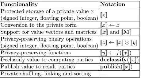
Functionality Notation
Protected storage of a private valuex [[x]] (signed integer, floating point, boolean)
Conversion to the private form [[x]]←x Support for value vectors and matrices [[x]] and [[M]] Privacy-preserving binary operations
[[z]]←[[x]]~[[y]] (signed integer, floating point, boolean)
Privacy-preserving functions [[y]]←f([[x]]) Declassify value to computing parties declassify([[x]]) Publish value to result parties publish([[x]]) Private shuffling, linking and sorting —
Table 1. Secure computation capabilities and notation for statistical analysis algo-rithms.
Specifically, we require the existence of the privacy-preserving operations listed in Table 1. The arithmetic operations are used for implementing statistical functions. Secure linking and sorting are required for preparing data tables for analysis. We also require a cryptographically private shuffling protocol that can randomly rearrange the values in a vector or rows in a matrix without leaking the elements being rearranged.
The threat models for different PDKs vary. For example, threats for a hardware-assisted PDK include backdoors and design flaws. For secure multi-party compu-tation, the main threat is that computing parties collude to reveal private inputs. PDKs also differ in their security assumptions and guarantees, e.g., they may remain private only when there is an honest majority, or withstand malicious tampering. Stronger security guarantees often come at a cost of computational power. Security against passive adversaries (who do not modify software but try to learn private values from its state) is sufficient for processing personal data when the computing parties are organizations with a legal responsibility to protect privacy.
One example of a practically feasible PDK is secure multi-party computation onadditively secret shared data [9]. If an input party wants to provide a secret value x ∈ Z (where Z is a quotient ring) as a private input to n computing parties, it uniformly generatesshares x1, . . . , xn−1←Z and calculates the final sharexn←x−x1− · · · −xn−1. Each computing party receives one sharexithat it stores as [[x]]. As an individual sharexi is just a uniformly distributed value, no computing party can learn anything about xwithout colluding with others.
Computing parties can process the shares without recovering the secret. For example, if each computing party has shares xi andyi of secretsxandy, they can calculatezi←xi+yi to get the shares ofz=x+y. Further operations in this protection domain kind require more complex protocols, as described in [9, 10]. The privacy and composability proofs for the cited protocols can be found in [6].
2.4 Limiting the leakage of private inputs
In our setting, data owners and analysts agree on a study plan, including what results can be published to the analysts. An ideal privacy goal would be to require that no information about the private inputs is revealed during the computations or in the outputs. However, this is impossible to achieve, as all practically useful outputs contain information about the private inputs.
Instead of forbidding leakage, we will use automatically enforced mechanisms to minimize it. We implementcontrolled statistics—our statistical tool will only publish results that the data owners and computing parties have cleared for pub-lishing. This approach has been shown to be a sufficient and legally acceptable way of protecting personal information and tax secrets in social studies [5].
The privacy-preserving algorithms in this paper are designed to minimize leakage using a combination of techniques that follow the following privacy goals.
Goal 1: Cryptographic security.During the evaluation of a function
([[y1]], . . . ,[[yk]])←f([[x1]], . . . ,[[xm]]),
want to prevent leaking private values through changes in the running time of the algorithm.
We achieve this goal as follows. First, our algorithms process all private values using composable secure operations in the PDK. This prevents leakage through any storage used by the computing party. Second, whenever possible, we design the algorithm as a straight line program. A straight line program consisting of universally composable secure operations is cryptographically secure and uni-versally composable itself [15]. Hence, we can omit the security proofs of such algorithms in this paper (Algorithms 3, 7, 8, 10, 14).
The remaining algorithms are not straight line programs and require separate security proofs. Most of these algorithms (Algorithms 1, 2, 4, 5, 6, 9) declassify the size of the selected subgroup, which is assumed to be public or is a desired output according to the study plan. We just optimize the running time by de-classifying certain results slightly earlier so that computing parties can reduce the amount of PDK operations they have to perform. For example, thecut func-tion reduces the amount of data to be processed by declassifying the size of the dataset that matches a search criterion, which is usually an allowable output in the study. Three remaining algorithms (Algorithms 11, 12, 13) declassify values that are independent of input data and thus privacy-preserving.
Fortunately, it is sufficient to analyse security in a hybrid model where ab-stract operations with private values reveal no information and an attacking computing party can make decisions only based on values that are declassified during the computations. Consequently, we must show that the transcript of val-ues declassified during runtime can be simulated knowing only the final published results of the algorithm. If this assumption is satisfied, then the implementation in the hybrid model can be shown to be cryptographically secure. As the compo-sition theorem from [15] assures that the security of the hybrid implementation does not degrade when we replace all abstract operations with the actual PDK operations. As long as all of them are universally composable, we have formally shown that our implementation is cryptographically secure.
Goal 2: Source privacy.An algorithm for computingf(x1, . . . , xm) is source-private if all outputs and all intermediate values do not depend on the order of inputs. If an algorithm for computing f(x1, . . . , xm) is cryptographically se-cure, it is sufficient to prove that the output distributions off(x1, . . . , xm) and
f(xπ(1), . . . , xπ(m)) coincide for all permutations of inputsπ.
Source privacy ensures that the computing parties are not capable of link-ing computation results with the private inputs of a specific input party. For instance, the simple sum x1+· · ·+xn is source private and, thus, it does not reveal the relation between input parties and their inputs even if we somehow know the values of x1, . . . , xn. The latter does not mean that we cannot infer something aboutxi. For instance, if all inputs are in a fixed range, the sum can limit the set of potential values ofxi. Similarly, we might get extra information aboutxi if we know some other valuesxj.
are independent of the inputs. All other statistical functions are independent on the order of inputs. Hence, it is straightforward to achieve source privacy by obliviously shuffling the inputs before the actual computations.
Goal 3: Query restrictions. A privacy-preserving statistical analysis system enforces query restrictions if it provides a mechanism for the input parties to control which computations can be performed by the computing parties on the private inputs and which results can be published to the result parties.
We achieve this goal by combining organizational controls with technical ones. First, the input parties negotiate a study plan that describes the compu-tations to be performed and their publishable results. Second, the study plan is implemented on theRmindtool using a PDK and the algorithms in this paper. Every result in the study plan is published using the publishoperation.
Rmindenforces these restrictions by requiring that computing parties have exactly the same version of the study plan deployed at the time of execution. The result party can only run queries for which the necessary algorithms are deployed. Parties cannot upload new code to perform any query. If at least one computing party refuses to run a query, it cannot be run. Input parties can have a greater control over the process, if they or their representatives also host a computing party.
Goal 4: Output privacy.A statistical study is output-private, if its published results do not leak the private inputs of the input parties.
Output privacy cannot be absolute, as this way we learn nothing from the pri-vate inputs. In practice, the amount of allowable leakage is strongly application-dependent. In the data integration scenario, data owners help compile the study plan and perform a privacy impact assessment of the publishable outputs. They can then decide to augment the algorithms with limitations. For example, they can require that a result cannot be published if it is a direct aggregation of, e.g., less than five, inputs. Also, they can limit the number of queries that can be sent to prevent the siphoning of private data.
Formal quantification of output privacy should be defined on well-founded mathematical formalisations likek-anonymity [54] and differential privacy [23]. Achieving these goals comes with the cost of reduced precision. The result parties must accept either noisy or coarse-grained results.
Legislations often specify requirements in terms equivalent or similar to k -anonymity, as it is easy to understand and verify such requirements. However, these privacy requirements do not protect against attackers with background information. Differential privacy guarantees security against attackers with un-bounded background knowledge, provided that the result parties are willing to accept a potentially unbounded amount of noise added to results [24].
typical statistical study, or otherwise the study would be redundant. Hence, dif-ferential privacy may provide overly conservative results by adding too much noise to outputs.
The authors conclude that the Rmind tool should have optional support for output randomisation techniques that one can use to achieve differential privacy. Moreover, defining a flavour of differential privacy that faithfully models the bounded nature of background information in statistical studies without inconsistencies is an important research goal.
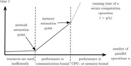
2.5 Achieving efficiency
Protection domain kinds may have specific performance profiles. For example, PDKs based on secret sharing, are significantly more efficient when the algo-rithms perform many parallel operations together. Figure 2 shows a generic running time profile for a secure multi-party computation operation [10].
performance is communication-bound
performance is CPU- or memory-bound time t
number of parallel operations n
resources are used network saturation
point
memory saturation
point
running time of a secure computation
operation
t = y(n)
iciently ineff
Fig. 2.Performance model of the secure computation protocols based on secret sharing.
The vertical axis shows the running timetof a secure multi-party computa-tion protocol based on secret sharing and the horizontal axis showsn, the number of simultaneous parallel operations. In the functiont=y(n),y characterises the running time of the protocol based on the network setting it is deployed in. A thorough study of functiony has been performed in [49].
much as possible in our algorithm design, utilizing batch processing to prevent exhausting computational resources.
We will allow the algorithm to optimize its running time, if this requires the declassification of a private value that is among the published outputs of the statistical function. For example, we will use aggregates like counts and sums to reduce the amount of data we have to process after certain filtering tasks.
3
Data import and filtering
We now present a collection of algorithms for performing privacy-preserving statistical analysis in the application model described in the previous sections. We begin with the first steps in the statistical analysis process—acquiring and preparing the data.
Data are crucial ingredients of statistical analyses and they can be collected for a specific designed study, such as a clinical trial. Alternatively, existing datasets can be used in analyses, e.g. tax data can be used to analyse the finan-cial situation of a country. We look at these two different methods separately as they entail special requirements in a privacy-preserving setting.
First, let us look at the case where data are collected for a specific study. In such studies, data are entered by a data collector (e.g. national census or a clinical trial) or by data donors themselves (e.g. an online survey) and the joint database is considered to be horizontally partitioned. With secure multi-party computation, the data are encrypted or secret-shared immediately at the source and stored in a privacy-preserving manner.
Second, consider the case where datasets previously exist and analysts wish to perform a study by combining data from several different databases that cannot be joined publicly into a newvertically partitioned database. Then, data can be imported from these databases by encrypting or secret-sharing them and later merging them in a privacy-preserving way.
For generality, we look at the data importing stage as one abstract operation. However, we keep in mind that when dealing with existing databases, data can be validated and filtered by the database owners and managers before they are imported into the privacy-preserving database. In addition to automatic checks, the data manager can also look at the data and see if there are questionable values that need to be checked or removed.
3.1 Availability mask vectors
The solution with an extra attribute is much more practical, as only one private bit of extra data needs to be stored per entry. The latter uses extra storage space ofN·k·bbits, whereN is the number of entries,kis the number of attributes, andbis the smallest data unit that can be stored in the database. In our work, we concentrate on the latter, as this allows us to perform faster computations on private data. Let the availability mask [[m]] of vector [[a]] contain 0 if the corresponding value in the attribute [[a]] is missing and 1 otherwise. It is clear, that it is not possible to discern which and how many values are missing from the value vector by looking at the private availability vector. However, the count of available elements can be computed by summing the values in the availability mask.
3.2 Input validation
By input validation and data correction, we mean operations that can be done without interacting with the user, such as range and type checks. The values for acceptable ranges and types are specified by the user but they are applied to the data automatically. Input validation and data correction can be performed at two stages—during data import on entered but not yet encrypted data, or afterwards, in the privacy-preserving database on encrypted data. It is, of course, faster, more sensible and straightforward to do this on data before encryption. If the data cannot be checked before encryption for some reason, the validation has to be performed in the privacy-preserving database.
To perform a range check on a private vector [[a]] of values, we construct a vector [[c]] containing the constant with which we want to compare the values. We then compare the two vectors point-wise and get a private vector [[m]] of comparison results, where [[mi]]←[[ai]]~[[ci]], where~is a comparison operation,
i ∈ {1, . . . , n}, andn is the size of vectors [[a]],[[c]] and [[m]]. Unlike the public range check operation, the privacy-preserving version does not receive as a result a private vector of values that are within range. Instead, it receives a mask vector [[m]] that can be used in further computations. To find out how many values are within range, it suffices to sum the values in vector [[m]].
3.3 Evaluating filters and isolating filtered data
Similarly to range checks, filtering can be performed by comparing a vector [[a]] of values point-wise to a vector [[c]] containing filter values. As a result, we obtain a mask vector [[m]] that contains 1 if the condition holds and 0 otherwise. For a more complex filter, the comparisons are done separately and the resulting mask vectors are combined using conjunction and disjunction.
Algorithm 1:Privacy-preserving functioncutfor cutting the dataset ac-cording to a given filter that leaks the size of the selected subset n.
Data: Data vector [[a]] of sizeN and corresponding mask vector [[m]]. Result: Data vector [[x]] of sizenthat contains only elements of [[a]]
corresponding to the mask [[m]]
1 Obliviously shuffle the value pairs in vectors ([[a]],[[m]]) into ([[a0]],[[m0]])
2 s←declassify([[m0]])
3 Form an output vector [[x]] by collecting all [[a0i]] for whichsi= 1 4 return[[x]]
conditions. To get the combined filter, we need to conjunct the filters together [[m]]←[[p]]∧[[q]]∧[[r]].
Most of the algorithms presented in this paper are designed so that filter information is taken into account during computations. On the other hand, some algorithms require that a subset vector containing only the filtered data be built. We use Algorithm 1 for selecting a subset based on a given filter in a privacy-preserving way.
First the value and mask vector pairs are shuffled in a privacy-preserving way, retaining the correspondence of the elements. Next, the mask vector is declassified and values for which the mask vector contains 0 are removed from the value vector. The obtained subset vector is then returned to the user. It is also possible to cut matrices in a similar fashion. This process leaks the number of values that correspond to the filter that the mask vector represents. If the number of records in the filter is published anyway, the functioncutdoes not reveal any new information, as oblivious shuffling ensures that no other information about the private input vector and mask vector is leaked [44].
Lemma 1. If operations in the PDK are universally composable, then Algo-rithm 1 leaks only the number of non-zero elements in the input mask filter.
Proof. In short, due to oblivious shuffle the elements ofsare in unknown random order. Hence, it is trivial to simulate the results of the declassify protocol—it suffices to fixnones in random locations.
Also, note that the order of shares [[x]] matches: if corrupted parties behave honestly, their shares of [[x]] are in the same order as specified by T. Conse-quently, the hybrid protocol is cryptographically secure. The security of the real implementation based on the PDK follows directly form the universal compos-ability of shuffle and declassify operations.
The availability of filtering, predicate evaluation and summing elements of a vector, allows us to implement privacy-preserving versions of data mining algorithms such as frequent itemset mining (FIM) [4]. As FIM is often used for mining sparse datasets, a significant speedup can be achieved if the infrequent itemsets are pruned using thecutfunction.
4
Data quality assurance
When databases are encrypted or secret-shared, the privacy of the data donor is protected and no users, including system administrators can see individual values. However, this also makes it impossible for the data analyst to see the data. Statistical analysts often detect patterns and anomalies, and formulate hypotheses when looking at the data values. Our solution is to provide privacy-preserving algorithms for a range of descriptive statistics that can give a feel of the data, while protecting the individual records.
Given access to these aggregate values and the possibility to eliminate out-liers, it is possible to ensure data quality without compromising the privacy of individual data owners. Even though descriptive statistics leak some information about inputs, the leakage is small and strictly limited to aggregations permitted on the current database.
4.1 Five-number summary
Box-plots are simple tools for giving a visual overview of the data and for effec-tively drawing attention to outliers. These diagrams are based on the five-number summary—a set of descriptive statistics that includes the minimum, lower quar-tile, median, upper quartile and maximum of an attribute. All of these values are, in essence, quantiles and can, therefore, be computed by using a formula for the appropriate quantiles. As no one method for quantile estimation has been widely agreed upon in the statistics community, we use algorithmQ7 from [35] used by the R software. Letpbe the percentile we want to find and let [[a]] be a vector of values sorted in ascending order. Then the quantile is computed using the following function:
Q(p,[[a]]) = (1−γ)·[[aj]] +γ·[[aj+1]] ,
Algorithm 2: Privacy-preserving algorithm for finding the five-number summary of a vector that leaks the size of the selected subset
Data: Input data vector [[a]] and corresponding mask vector [[m]].
Result: Minimum [[min]], lower quartile [[lq]], median [[me]], upper quartile [[uq]], and maximum [[max]] of [[a]] based on the mask vector [[m]]
1 [[x]]←cut([[a]],[[m]])
2 [[b]]←sort([[x]])
3 [[min]]←[[b1]]
4 [[max]]←[[bn]] 5 [[lq]]←Q(0.25,[[b]])
6 [[me]]←Q(0.5,[[b]])
7 [[uq]]←Q(0.75,[[b]])
8 return([[min]],[[lq]],[[me]],[[uq]],[[max]])
Algorithm 3: Privacy-preserving algorithm for finding the five-number summary of a vector that hides the size of the selected subset.
Data: Input data vector [[a]] of sizeN and corresponding mask vector [[m]]. Result: Minimum [[min]], lower quartile [[lq]], median [[me]], upper quartile [[uq]],
and maximum [[max]] of [[a]] based on the mask vector [[m]]
1 ([[b]],[[m0]])←sort∗([[a]],[[m]])
2 [[n]]←sum([[m]])
3 [[os]]←N−[[n]]
4 [[min]]←[[b[[1+os]]]]
5 [[max]]←[[bN]]
6 [[lq]]←Q∗(0.25,[[a]],[[os]])
7 [[me]]←Q∗(0.5,[[a]],[[os]])
8 [[uq]]←Q∗(0.75,[[a]],[[os]])
9 return([[min]],[[lq]],[[me]],[[uq]],[[max]])
Using the quantile computation formula Q, the five-number summary can be computed as given in Algorithm 2. The algorithm uses Algorithm 1 to re-move unwanted or missing values from the data vector. The subset vector is sorted in a privacy-preserving way and the summary elements are computed. As mentioned before, function cut leaks the count of elements nthat correspond to the filter signified by the mask vector [[m]]. If we want to keep n secret, we can use Algorithm 3 which hides n, but is slower than Algorithm 2. Note that Algorithm 2 consists of thecut operation followed by a straight line program. Hence, we can use the universal composability property of the PDK together with the cut security proof to conclude that Algorithm 2 is cryptographically secure.
Algorithm 4:Privacy-preserving algorithm for finding the frequency table of a data vector that leaks the size of the selected subset.
Data: Input data vector [[a]] and corresponding mask vector [[m]].
Result: Vector [[b]] containing breaks against which frequency is computed, and vector [[c]] containing counts of elements
1 [[x]]←cut([[a]],[[m]])
2 n←size([[x]])
3 k← dlog2(n) + 1e
4 [[min]]←min([[x]]), [[max]]←max([[x]])
5 Securely compute breaks [[b]] according to [[min]],[[max]] andk
6 [[ci]]←(sum([[xi]]≤[[bi+1]]), i∈ {1, . . . , n})
7 fori∈ {k, . . . ,2}do
8 [[ci]]←[[ci]]−[[ci−1]]
9 end
10 return([[b]],[[c]])
quantiles works asQwith the exception that, as the number of elements [[n]] is kept private, the indices [[j]] are also not revealed. The computed offset [[os]] is added to the private index [[j]] to account for the values at the beginning of the sorted vector that do not belong to the filtered subset. In addition, vector lookup on line 4 and during the computations of the quantiles are now performed in a privacy-preserving way. As a result, the value is retrieved while the the index remains secret for all computing parties.
4.2 Data density estimation
The distribution of values of an attribute gives an insight into the data. For cate-gorical attributes, the distribution can be discerned by counting the occurrences of different values. For numerical attributes, we must split the range into bins specified by breaks and compute the corresponding frequencies. The resulting frequency tables can be visualised as a histogram.
Algorithm 4 computes a frequency table for a vector of numerical values similarly to a public frequency computation algorithm. Missing or filtered values are removed on line 1. The sizenof the returned vector [[x]] is determined by the functionsizeon line 2. As we do not hide the sizes of private vectors, this function returns a public value. The number of binskis publicly computed according to Sturges’ formula [52]. Bins are created in a privacy-preserving manner based on the minimum, maximum andk. Finally, on lines 6 - 9, the elements belonging in each bin are counted using secure multi-party computation. These comparisons can be done in parallel to speed up the algorithm.
4.3 Simple statistical measures
Statistical algorithms use common operations for computing means, variance and covariance. These statistical measures also provide important insights about the attributes and their correspondence. We show, how these measures can be computed in a privacy-preserving manner over various samples.
To compute means, variances and covariances, we first multiply point-wise the value vector [[a]] of sizeNwith the mask vector [[m]]. Let us denote the result by [[x]]. This way, the values that do not correspond to the filter do not interfere with the computations. The number of subjects [[n]] is computed by summing the elements in the mask vector. The arithmetic mean, and the unbiased estimates of variance and standard deviation can be computed as follows
mean([[x]]) = 1 [[n]]·
N X i=1
[[xi]] ,
var([[x]]) = 1 [[n]]−1
N X i=1
[[xi]]2− 1 [[n]]·
N X i=1
[[xi]] !2
,
sdev([[x]]) =pvar([[x]]) .
The computation of these values is straightforward, if the privacy-preserving platform supports addition, multiplication, division and square root. Further-more, ifnis public, we can use division with a public divisor and public square root instead, as they are faster than the private versions.
Trimmed mean is a version of mean where the upper and lower parts of the sorted data vector [[a]] are not included in the computation. The analyst specifies the percentage of data that he or she wants to trim off the data. Then the corresponding quantiles are computed, data are compared to these values and the mask vector [[m]] is updated with the results acquired from the comparison operation. This ensures that only values that fall between the given percentages remain in the filtered result [[x]].
Covariance shows whether two attributes change together. The unbiased es-timate of covariance between filtered vectors [[x]] and [[y]] can be computed as
cov([[x]],[[y]]) = 1 [[n]]−1
N X i=1
[[xi]][[yi]]− 1 [[n]]·
N X i=1
[[xi]] N X i=1
[[yi]] !
.
4.4 Univariate outlier detection
Datasets often contain errors or extreme values that should be excluded from the analysis. Although there are many elaborate outlier detection algorithms like [13], outliers are often detected using quantiles.
computed by comparing all elements of [[a]] toQ(0.05,[[a]]) andQ(0.95,[[a]]), and then conjuncting the resulting index vectors.
The values of the quantiles need not be published for outlier detection pur-poses and data are filtered to exclude outliers from further analysis. Furthermore, it is possible to combine the mask vector with the availability mask [[m]] and cache it as an updated availability mask to reduce the filtering load.
Another generic measure of eliminating outliers from a dataset is using me-dian absolute deviation [30, 31] (MAD). Element [[x]] is considered an outlier in a value vector [[a]] of length nif
|Q(0.5,[[a]])−[[x]]|> λ·MAD,
where
MAD=Q(0.5,|[[ai]]−Q(0.5,[[a]])|) , i∈ {1, . . . , n}
andλis a constant. The exact value of λis generally between 3 to 5, but it can be specified depending on the dataset.
5
Statistical tests
It is often useful to compare behaviours in two groups, often referred to as the case and control populations. There are two ways to approach this. Firstly, we can select the appropriate subjects into one group and assume all the rest are in the other group. Alternatively, we can choose subjects into both groups. These selection categories yield either one or two mask vectors. In the former case, we compute the second mask vector by flipping all the bits in the existing mask vector. Hence, we can always consider the version where case and control groups are determined by two mask vectors.
In the following, let [[a]] be the value vector we are testing and let [[ca]] and [[co]] be mask vectors for case and control groups, respectively. Then [[nca]] = sum([[ca]]) and [[nco]] =sum([[co]]) are the counts of subjects in the correspond-ing populations.
5.1 The principles of statistical testing
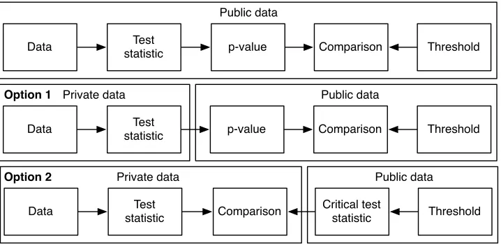
Figure 3 gives an overview of what the different steps are for statistical testing in the private and public setting. In a normal statistical testing procedure, we first compute the test statistic based on the data. Next, we compute the p-value based on the obtained value and the size of the sample. Finally, we compare the p-value to a significance threshold set by the analyst.
In the privacy-preserving setting, we have two options of how to carry out this procedure. The choice depends on how much information we are willing to publish.
Public data
Data statisticTest p-value Threshold
Public data
Data Test
statistic p-value Threshold
Private data
Comparison
Comparison
Public data
Data statisticTest Critical teststatistic Threshold
Private data
Comparison Option 1
Option 2
Fig. 3.Statistical testing procedure in the public and private setting
given threshold value. As the function that converts the test statistic to into the p-value is always monotone and depends only on the sizes of case and control groups. Consequently, it can be always inverted if sample sizes are public. Hence, publishing the test statistic is equivalent to revealing the p-value together with the sizes of case and control groups.
However, revealing the sizes of the case and control groups or the raw p-value might sometimes reveal too much information. For this occasion, we propose Option 2, where the test statistic is computed based on the data in a privacy-preserving manner. The data analyst determines the threshold, and the critical p-value and the corresponding test statistic are publicly determined based on this threshold. Finally, the private test statistic is compared to the critical test statistic in a privacy-preserving manner. The only thing that is published is the decision whether the alternative hypothesis is supported by the data.
We discuss how to perform Student’s t-test, paired t-test, Wilcoxon rank sum and signed-rank tests, and theχ2test in a privacy-preserving manner. These test algorithms return the test statistic value that has to be combined with the sizes of the compared populations to determine the significance of the difference.
5.2 Student’s t-tests
of the control population. For equal variance, the t-test statistic is computed as:
[[t]] = mean([[x]])−mean([[y]]) sdev([[x]],[[y]])·q 1
[[nca]]+ 1 [[nco]]
,
wheresdev([[x]],[[y]]) estimates the common standard deviation of the two sam-ples and is computed as follows
sdev([[x]],[[y]]) = s
([[nca]]−1)·var([[x]]) + ([[nco]]−1)·var([[y]]) [[nca]] + [[nco]]−2
.
The t-test for unequal variances is also known as the Welch t-test. The test statistic is computed as follows
[[t]] =mean([[q x]])−mean([[y]])
var([[x]]) [[nca]] +
var([[y]]) [[nco]]
.
A paired t-test [39] is used to detect whether a significant change has taken place in cases where there is a direct one-to-one dependence between case and control group elements, for example, the data consists of measurements from the same subject. Let [[x]] and [[y]] be the paired measurements, and letnbe the count of these measurements. The test statistic for the paired t-test is computed in the following way
[[t]] = mean([[x]]−[[y]])· p
[[n]] sdev([[x]]−[[y]]) .
The algorithms for computing both t-tests are straightforward evaluations of the respective formulae using privacy-preserving computations. To compute these, we need the availability of privacy-preserving addition, multiplication, division and square root. As mentioned earlier, we can either publish the test statistic and the population sizes or, based on a user-given threshold, publish only whether the hypothesis was significant or not.
5.3 Wilcoxon rank sum test and signed rank test
Algorithm 5: Privacy-preserving two-sided Mann-Whitney U test that leaks the total size of the case and control group
Data: Value vector [[a]] and corresponding mask vectors [[ca]] and [[co]] Result: Test statistic [[w]]
1 [[m]]←[[ca]]∨[[co]]
2 [[nca]]←sum([[ca]]) and [[nco]]←sum([[co]]) 3 ([[x]],[[u]],[[v]])←cut(([[a]],[[ca]],[[co]]),[[m]])
4 ([[x]],[[u]],[[v]])←sort([[x]],[[u]],[[v]])
5 [[r]]←rank([[x]])
6 [[rca]]←[[r]]·[[u]] and [[rco]]←[[r]]·[[v]]
7 [[Rca]]←sum([[rca]])
8 [[uca]]←[[Rca]]−12([[nca]]·([[nca]] + 1)) and [[uco]]←[[nca]]·[[nco]]−[[uca]] 9 return[[w]]←min([[uca]],[[uco]])
Algorithm 6:Privacy-preserving Wilcoxon signed-rank test that leaks the size of the case and control group
Data: Paired value vectors [[a]] and [[b]] fornsubjects, mask vector [[m]] Result: Test statistic [[w]]
1 ([[x]],[[y]])←cut(([[a]],[[b]]),[[m]])
2 [[d]]←[[x]]−[[y]]
3 Let [[d0]] be the absolute values and [[s]] be the signs of elements of [[d]]
4 [[s]]←sort(([[d0]],[[s]]))
5 [[r]]←rank0([[s]])
6 return[[w]]←sum([[s]]·[[r]])
functioncut is the same as before, except that several vectors are cut at once based on the combined filter [[m]]. Next, the value and mask vectors are sorted based on the values of [[x]] so that the relation between the values and mask elements is retained.
Therankfunction on line 5 shares and assigns an integer i∈ {1, . . . , n} to all values in the sorted vector based on the location of the value. If some values in the sorted vector are equal, all of these elements are assigned the average of their ranks. This is done using oblivious comparison and oblivious division. This correction makes the algorithm significantly slower as this requires us to keep all the ranks as floating point values instead of integers. It is possible to use this test without the correction which makes it give a stricter bound and might not accept borderline hypotheses, but the algorithm will work faster. On line 6, the rank vector [[r]] is multiplied with the case and control masks to find the ranks belonging to the case and control groups.
Similarly to Student’s paired t-test, the Wilcoxon signed-rank test [55] is a paired difference test. Our version, given in Algorithm 6, takes into account Pratt’s correction [34] for when the values are equal and their difference is 0.
is found, followed by the computation of the absolute value and sign of [[d]]. We expect that the latter is the standard function that returns−1 when the element is negative, 1 if it is positive and 0 otherwise. The signs are then sorted based on the absolute values [[d0]] (line 4) and the ranking functionrank0 is called.
This ranking function is otherwise similar to the function rank, but differs in the fact that we also need to exclude the differences that have the value 0. Let the number of 0 values in vector [[d]] be [[k]]. As [[d]] has been sorted based on absolute values, the 0 values are at the beginning of the vector so it is possible to use [[k]] as the offset for our ranks. Function rank0 assigns [[ri]] ← 0 while [[si]] = 0, and works similarly to rank on the rest of the vector [[s]], with the difference thati∈ {1, . . . ,[[n−k]]}.
Both algorithms only publish the statistic value and the population sizes. As the first operationcutis followed by a straight line program in both algorithms, the universal composability property of the PDK together with the security proof of functioncutis sufficient for concluding cryptographic security of both algorithms.
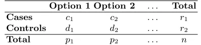
5.4 The χ2 tests for consistency.
If the attribute values are discrete such as income categories then it is impossible to apply t-tests or their non-parametric counterparts and we have to analyse frequencies of certain values in the dataset. The corresponding statistical test is known as the χ2 test. The standardχ2 test statistic is computed as
χ2= k X i=1
m X j=1
(fji−eji)2
eji
,
wherefjiis the observed frequency andejiis the expected frequency of thei-th option andj-th group. As we are working with two populations, we can simplify this formula as
χ2= k X
i=1
(ci−e1i)2
e1i
+(di−e2i) 2
e2i
,
then the frequencies can be presented as the contingency Table 2.
To give the analyst the possibility to choose, which values will be converted into which option in the contingency table, we introduce the notion of a public codebookCB. This matrix essentially holds the possible values of the attribute in the first column, and the option they will belong to, in the second.
Option 1 Option 2 . . . Total
Cases c1 c2 . . . r1
Controls d1 d2 . . . r2
Total p1 p2 . . . n
Algorithm 7:Privacy-preserving algorithm for compiling the contingency table for two classes withk options for theχ2 test
Data: Value vector [[a]], corresponding mask vectors [[ca]] and [[co]] for cases and controls respectively and a public code bookCBdefiningkoptions fromupossible values of the attribute
Result: Contingency table [[CT]]
1 [[xca]]←[[a]]·[[ca]] and [[xco]]←[[a]]·[[co]] 2 Let [[CT]] be a 2×k matrix
3 fori∈ {1, . . . , u}do
4 [[bca]]←[[xca]] =CBi,1and [[bco]]←[[xco]] =CBi,1
5 j←CBi,2
6 [[CT1,j]]←[[CT1,j]] +sum([[bca]]) 7 [[CT2,j]]←[[CT2,j]] +sum([[bco]]) 8 end
9 return[[CT]]
Algorithm 8: Privacy-preservingχ2 test of independence Data: Contingency table [[C]] of size 2×k
Result: The test statisticχ2
1 Let [[n]] be the total count of elements
2 Let [[r1]] and [[r2]] be the row subtotals and [[p1]], . . . ,[[pk]] be the column subtotals 3 Let [[E]] be a table of expected frequencies such that
[[Ei,j]]←
[[ri]]·[[pj]]
n ,i∈ {1,2}, j∈ {1, . . . , k} 4 [[χ2]]←
P
jk=1 ([[C1,j]]−[[E1,j]])2
[[E1,j]] +
([[C2,j]]−[[E2,j]])2 [[E2,j]] 5 return[[χ2]]
Algorithm 7 compiles a contingency table from a data vector, mask vector and the public code bookCB. Algorithm 8 shows how to compute theχ2 test statistic based on a contingency table. The algorithm can be optimised if the number of classes is small, e.g. two. The algorithm publishes only the statistic value and the population sizes.
5.5 Multiple testing
Algorithm 9: Privacy-preserving Benjamini-Hochberg procedure Data: Vector ofk test statistics [[t]], significance thresholdα
Result: List of significant hypotheses
1 Publicly computeq(i)≈Q iαk
fori∈ {1, . . . , k}.
2 Obliviously sort pairs ([[ti]],[[i]]) in descending order wrt. [[ti]]. 3 Let ([[t(i)]],[[c(i)]]) be the result.
4 Compute [[si]]←([[t(i)]]≥q(i)) fori∈ {1, . . . , k}.
5 Declassify values [[sk]],[[sk−1]], . . .[[s1]] until the first 1 ([[si∗]] = 1) is revealed.
6 Declassify locations [[c(1)]], . . . ,[[c(i∗)]]. Declare these hypotheses significant.
Bonferroni correction. Letαbe the significance threshold and let k be the number of tests applied on the same data. Then the Bonferroni correction simply reassigns the same significance threshold ˆα = α/k to all tests. As a result, Bonferroni correction is trivial to implement, we just have to use the corrected significance threshold ˆαof all privacy-preserving statistical tests.
Benjamini-Hochberg procedure. Bonferroni correction is often too harsh compared to false discovery rate (FDR) correction. Unfortunately, FDR is not as straightforward to apply in the privacy-preserving setting as for multiple testing p-values must remain private. Therefore, we look at the Benjamini-Hochberg (BH) procedure [2]. The BH procedure first orders p-values in ascending order and then finds the largestisuch that
p(i)≤
i kα
wherep(i)is thei-th p-value andkis the number of hypotheses.
Recall that for any statistical test the correspondence between between p-values and test statistics is anti-monotone. Namely, for any significance threshold
αwe can find a valueQ(α) such that for any value of the test statistict≥Q(α) the corresponding p-value is less than α. As a result, the Benjamini-Hochberg criterion can be expressed in terms of decreasingly ordered test statistics:
p(i)≤
i
kα ⇐⇒ t(i)≥Q
iα
k
.
For most tests, the functionQis computed as the upper quantile of a distri-bution that depends only on the size of the case and control group. Hence, we can publicly compute fractional approximations of significance thresholds
q(i)≈Q
iα k
and use secure computing to evaluate comparisons t(i)≥q(i).
statistics. It is even possible to hide the ordering if the shares [[c(1)]], . . . ,[[c(i∗)]] are
obliviously shuffled before opening such thatc(1), . . . , c(i∗)are opened in random
order. As the number of revealed zeroes is equal to the number of significant hy-potheses, we can directly simulate the published values knowing only the desired outcome. The formal security proof is analogous to the proof of Lemma 1.
6
Predictive modelling
As most prediction models are defined in terms of linear algebra, we have im-plemented privacy-preserving versions of the following vector and matrix opera-tions: computing the dot product, computing vector length, computing the unit vector, and matrix multiplication. It is also possible to transpose a matrix and compute its determinant. In addition, we have implemented cross product for vectors of length 3, and eigenvector and eigenvalue computation for 2×2 sym-metric matrices. The privacy-preserving versions of these algorithms are straight-forward and can be used in linear regression models.
6.1 Linear regression
Linear regression is the most commonly used method for predicting values of variables based on other existing variables. It can also be used to find out if and how strongly certain variables influence other variables in a dataset.
Let us assume that we havekindependent variable vectors ofnelements, i.e X= (Xj,i), wherei∈ {0, . . . , k}andj∈ {1, . . . , n}. The vectorXj,0= (1) is an added variable for the constant term. Let y= (yj) be the vector of dependent variables. We want to estimate the unknown coefficientsβ= (βi) such that
yj=βkXj,k+. . .+β1Xj,1+β0Xj,0+εj
where the vector of errorsε= (εj) is assumed to be white Gaussian noise. This list of equations can be compactly written as ε =Xβ−y. Most methods for linear regression try to minimize the square of residuals
kεk2=ky−Xβk2 . (1)
This can be done directly or by first converting the minimization task into its equivalent characterization in terms of linear equations:
XTXβ=XTy . (2)
Let us first look at simple linear regression, where the aim of the analysis is to find ˆα and ˆβ that fit the approximationyi ≈β0+β1xi best for all data points. Then the corresponding linear equation (2) can be solved directly:
ˆ
β1=
cov(x,y) var(x) ˆ
Algorithm 10: maxLoc: Finding the first maximum element and its lo-cation in a vector in a privacy-preserving setting
Data: A vector [[a]] of lengthn
Result: The maximum element [[b]] and its location [[l]] in the vector
1 Letπ(j) be a permutation of indicesj∈ {1, . . . , n} 2 [[b]]←[[aπ(1)]] and [[l]]←π(1)
3 fori∈ {π(2), . . . , π(n)}do
4 [[c]]←([[aπ(i)]] >|[[b]]|)
5 [[b]]←[[b]]−[[c]]·[[b]] + [[c]]·[[aπ(i)]]
6 [[l]]←[[l]]−[[c]]·[[l]] + [[c]]·π(i)
7 end
8 return([[b]],[[l]])
As we have the capability to compute covariance and variance in the privacy-preserving setting, we can also estimate the values of ˆβ0 and ˆβ1 in this setting.
We will look at three different methods for solving the system (2) with more than one explanatory variable: for k <4, we simply invert the matrix by com-puting determinants. For the general case, we give algorithms for the Gaussian elimination method [48] and LU decomposition [48]. We also describe the con-jugate gradient method [33] that directly minimizes the square of residuals (1). In all these algorithms, we assume that the data matrix has already been multiplied with its transpose: [[A]] = [[X]]T[[X]] and the dependent variable has been multiplied with the transpose of the data matrix: [[b]] = [[X]]T[[y]].
In the privacy-preserving setting, matrix inversion using determinants is straightforward, and using this method to solve a system of linear equations requires only the use of multiplication, addition and division, and, therefore, we will not discuss it in length. For the more general methods for solving systems of linear equations, we first give an algorithm that finds the first maximum el-ement in a vector and also returns its location in the vector, used for finding the pivot element. While the Gaussian and LU decomposition algorithms can be used without pivoting, it is not advisable as the algorithms are numerically unstable in the presence of any roundoff errors [48].
Of the two algorithms for solving a system of linear equations, let us first look more closely at Gaussian elimination with backsubstitution. Algorithm 11 gives the privacy-preserving version of the Gaussian elimination algorithm.
At the start of the algorithm (line 2), the rows of the input matrix [[A]] are shuffled along with the elements of the dependent variable vector, that have been copied to [[x]], retaining the relations. On lines 5-13, the pivot element is located from the remaining matrix rows and then the rows are interchanged so that the one with the pivot element becomes the current row. Note that all the matrix indices are public and, hence, all of the conditionals work in the public setting. As we need to use the pivot element as the divisor, we need to check whether it is 0. However, we do not want to give out information about the location of this value so, on line 14, we privately make a note whether any of the pivot elements is 0, and on line 34, we finish the algorithm early if we are dealing with a singular matrix. Note that in the platform we are using, division by 0 will not be reported during privacy-preserving computations as this would reveal the divisor immediately.
On lines 17 22, elements on the pivot line are reduced. Similarly, on lines 23 -31, elements below the pivot line are reduced. Finally, on lines 36 - 39, backsub-stitution is performed to get the values of the coefficients.
The main difference between the original and the privacy-preserving Gaussian elimination algorithm is actually in themaxLocfunction. In the original version, elements are compared one-by-one to the largest element so far and at the end of the subroutine, the greatest element and its location have been found. As for our system, we basically do the same thing only we use oblivious choice instead of the straightforward if-clauses. This way, we are able to keep the largest element secret and we only reveal its location at the end without finding out other relationships between elements in the vector during the execution of this algorithm.
Lemma 2. If operations in the PDK are universally composable, then Algo-rithm 11 leaks only whether the matrix is singular or not.
Proof. During the execution of the algorithm, row indicespiof pivoting elements are declassified to computing parties. For the proof, we must show that pivoting indexp= (pi) leaks no information about the matrixA.
For technical reasons, it is better to represent p in terms of original row labels. For that, we initially label rows of A after the shuffling with 1, . . . , n
and carry these labels through the computations. Hence,pi is not equal to the declassified output of themaxLocoperation. Instead,pi is the original label of the row after shuffling. For example, let the first maximum element be in row 4. Then pi = 4, the first and fourth rows are interchanged and the matrix is reduced. During the next step, let the maximum element be again in row 4. Now
Algorithm 11:Privacy-preserving Gaussian elimination with backsubsti-tution for a matrix equationAx=bthat leaks if the matrix is singular
Data: ak×kmatrix [[A]], a vector [[b]] ofkvalues Result: Vector [[x]] of coefficients
1 Let [[x]] be a copy of [[b]]
2 Obliviously shuffle [[A]],[[x]] retaining the dependencies
3 Let [[c]]←falseprivately store the failure flag during execution 4 fori∈ {1, . . . , k−1}do
5 [[m]] be a subvector of [[Au,v]] such thatu∈ {i, . . . , k}, v=i 6 ([[t]],[[irow]])←maxLoc([[m]])
7 irow←declassify([[irow]]) +i
8 if irow6=ithen
9 forj∈ {1, . . . , k}do
10 Exchange elements [[Airow,j]] and [[Ai,j]]
11 end
12 Exchange element [[xirow]] and [[xi]]
13 end
14 [[c]]←[[c]]∨([[Ai,i]] = 0) 15 [[pivinv]]←[[Ai,i]]−1 16 [[Ai,i]]←1
17 forj∈ {1, . . . , k}do
18 if j6=ithen
19 [[Ai,j]]←[[Ai,j]]·[[pivinv]]
20 end
21 [[xi]]←[[xi]]·[[pivinv]]
22 end
23 form∈ {i+ 1, . . . , k}do
24 forj∈ {1, . . . , k}do
25 if j6=ithen
26 [[Am,j]]←[[Am,j]]−[[Ai,j]]·[[Am,i]]
27 end
28 end
29 [[xm]]←[[xm]]−[[xi]]·[[Am,i]] 30 [[Am,i]]←0
31 end
32 end
33 if declassify([[c]])then
34 return”Singular matrix” 35 end
36 [[xk]]← [[xk]] [[Ak,k]]
37 fori∈ {k−1, . . . ,1}do
38 [[xi]]←[[xi]]− k
P
j=i+2
[[Ai,j]]·[[xj]] 39 end
steps are deterministic, as there is only one element with maximal absolute value larger than zero form. In this case, we can always obtainA∗ by permuting the rows ofA. This claim clearly holds, at the beginning of execution. Now assume that the claim holds at the beginning of the for-cycle (line 4). Then vectorsm and m∗ will contain the same elements. Consequently, both algorithms must choose the row with the same matrix elements. The following reduction steps of the algorithm use this row to modify remaining rows. As the set of rows to be modified is the same up to the permutation of rows, the reduction step yields the same results up to the row permutation. This completes the induction.
If there are several equal maximal elements then the pivoting indexpis not uniquely determined by the matrices AandA∗. Nevertheless, we can compare the distributions of p and p∗. We do this by carefully aligning runs of both algorithms. We can represent such runs by the tree of events where intermediate decision nodes represent choices made by themaxLocalgorithm. AsmaxLoc chooses elements with the maximal absolute value with equal probability, each child is chosen uniformly when we reach such a decision node. Note that up to the first equality the claim about matricesAandA∗ still holds. As the order of children in the decision node does not alter probabilities, we can align event trees so that the children match. As a result, the row with the same element is chosen in matching children and thus matrix A∗ can be still obtained by permuting the rows ofA∗. Hence, both runs of the algorithms can be represented with the same event tree such that A∗ in each leaf node can be obtained by permuting the rows ofA.
Note that if we assign row labels to A before shuffling, then the pivoting indicespandp∗ will be identical in each leaf node. Consequently, the distribu-tions of pivoting indices will be the same. As the indices are assigned after the shuffling step, we can obtain the distribution of p by taking p∗ and applying a random permutation π to all elements, i.e., pi = π(p∗i). The latter directly implies thatpis distributed as a uniform permutation.
The claim holds even if the matrix is singular and thus someAi,i= 0. If the inversion operation returns a fixed value as 0−1 all claims presented above still hold. If the inversion operation returns several values with different probabilities, then we must add additional decision nodes to the event tree. The latter, does not change the reasoning, as choices can be matched similarly to before. Hence, we get matching event trees and the claim still holds. For the same reason, the claim holds even if all arithmetical operations are imprecise and probabilistic.
To complete the proof, we must formally define the corresponding simulator construction. The latter is straightforward. We first sample the pivoting index pand then simulate shares to match the execution dictated by p. We omit the construction here as it is analogous to the simulator construction in Lemma 1.
Algorithm 12: LUDecomp: Privacy-preserving LU decomposition for a symmetric matrix Athat leaks if the matrix is singular
Data: ak×kmatrix [[B]]
Result: The LU decomposition matrix [[B]] andqcontaining the row permutations
1 Let [[c]]←0 be a boolean value
2 fori∈ {1, . . . , k}do
3 [[m]] be a subvector of [[Bu,v]] such thatu∈ {i, . . . , k}, v=i 4 ([[t]],[[irow]])←maxLoc([[m]])
5 irow←declassify([[irow]])
6 if irow6=ithen
7 forj∈ {1, . . . , k}do
8 Exchange elements [[Birow,j]] and [[Bi,j]]
9 end
10 end
11 [[c]]←[[c]]∨([[Bi,i]] = 0) 12 qi←irow
13 [[ipiv]]←[[Bi,i]]−1
14 form∈ {i+ 1, . . . , k}do
15 [[Bm,i]]←[[Bm,i]]·[[ipiv]] 16 forj∈ {i+ 1, . . . , k}do
17 [[Bm,j]]←[[Bm,j]]−[[Bm,i]]·[[Bi,j]]
18 end
19 end
20 end
21 if declassify([[c]])then
22 return”Singular matrix”
23 end
24 return([[B]],q)
to the process we used in the Gaussian elimination method. Algorithm 12 gives the privacy-preserving version of LU decomposition. Note, that the elements on the diagonal of the lower triangular matrix L are equal to 1. Knowing this, L andUcan be returned as one matrix such that the diagonal and elements above it belong to the upper triangular matrixUand the elements below the diagonal belong to the lower triangular matrixL without losing any information.
Similarly to Algorithm 11, first the pivot element is found using themaxLoc function. After the elements are exchanged, the row permutations are saved for use in the algorithm for solving the set of linear equations. As a result, the decomposition matrix and the permutations are returned. The permutations are public information but they reveal nothing about the original dataset because the rows have been shuffled before inputting them to the decomposition algorithm similarly to what was done in Algorithm 11.
Algorithm 13: Solving linear regression task y ≈Xβ using the LU de-composition matrix in a privacy-preserving setting
Data: An n×kdata matrix [[X]] and annelement response vector [[y]] Result: A vector [[b]] of coefficients
1 Compute correlation matrix [[A]]←[[X]]T[[X]] 2 Compute new target vector [[b]]←[[X]]T[[y]]
3 Shuffle [[A]],[[b]] retaining the dependencies
4 ([[B]],q)←LUDecomp([[A]])
5 Rearrange [[b]] based on permutationq 6 fori∈ {2, . . . , k}do
7 [[bi]]←[[bi]]− i
P
j=1
[[Bi,j]]·[[bj]] 8 end
9 fori∈ {k, . . . ,1}do
10 [[bi]]← [[bi]]− k
P
j=i+1
[[Bi,j]]·[[bj]]
!
·[[Bi,i]]−1 11 end
12 return[[b]]
Proof. This reasoning is the same as for Lemma 2. It is easy to see that both algorithms output the same pivoting vectors, as the sub-matrix used for choosing the pivot row is updated identically in both algorithms.
Algorithm 13 shows how to solve a set of linear equations using LU position. The matrix rows are shuffled as in Algorithm 11 and the LU decom-position matrix is composed using the LUDecompfunction. As an additional result we receive the permutation that was done for pivoting purposes during the decomposition phase. Next, on row 5, elements of the vector [[b]] containing the dependent variable are permuted to be in concurrence with the permuta-tions that were performed during the decomposition phase. In the usual setting, this step does not need to be done, as the elements can be accessed on the fly using the permutation vectorq, but in the privacy-preserving setting, it is more feasible to first rearrange the vector and then access the elements in order.
On rows 6 - 8, forward substitution is performed using the values from the lower triangular matrix. Finally, on rows 9 - 11, backsubstitution is performed using the values from the upper triangular matrix.
For the security consideration, note that Lemma 3 assures that line 4 is universally composable and, thus, the entire algorithm is a straight line program consisting of universally composable operations. As such, it is also secure.
Algorithm 14:Privacy-preserving conjugate gradient method
Data: ak×kmatrix [[A]] = [[X]]T[[X]], a vector [[b]] = [[X]]T[[y]] ofkvalues for
the dependent variable, public number of iterationsz Result: A vector [[x]] of coefficients
1 Let [[x]] be a vector ofk values 0
2 [[x]]←[[x]]T
3 [[r]],[[p]]←[[b]]
4 repeat
5 [[α]]← [[r]] T[[r]] [[p]]T[[A]][[p]]
6 [[x]]←[[x]] +α[[p]]
7 [[s]]←[[r]]−α[[A]][[p]]
8 [[β]]← [[s]] T[[s]] [[r]]T[[r]]
9 [[p]]←[[s]] + [[β]][[p]]
10 [[r]]←[[s]]
11 z←z−1
12 untilz = 0;
13 return[[x]]T
kis the number of columns in the matrixA, provided that all computations are done without errors [1].
As our matrix is symmetric and positive semi-definite, we can use the sim-plest version of this method with the fixed number of iterations that depends on the number of variablesk. Considering that the initial convergence of the conju-gate gradient method is rapid during a small number of iterations [1] and that privacy-preserving floating point operations are approximately as imprecise as operations with the float datatype in the normal setting, we decided to use fixed number of iterations in all of our experiments. As the largest number of variables was 10, the number of iterations was fixed to 10. Algorithm 14 shows how to solve our quadratic programming task using the conjugate gradient method. As Algorithm 14 is a straight line program, it is secure by default.
7
The implementation of Rmind
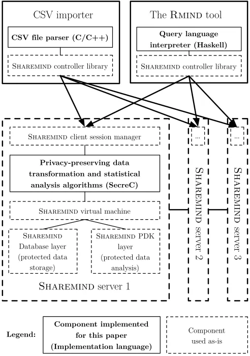
7.1 Implementation architecture
We have built an implementation of the privacy-preserving statistical analy-sis tool on the Sharemind secure computation framework [3]. We used the
additive3pp PDK originally introduced in [9] as the computation backend. In
this setting, no computing partyCP can derive information about intermediate values unless it colludes with another computing party.
Figure 4 shows the architecture of the tool and how differentSharemind com-ponents were used in its implementation.
ile parser (C/C++)
Sharemind
serv
er 2
CSV importer
Sharemind controller library
The Rmind tool
Sharemind controller library
Sharemind server 1
Sharemind client session manager
Sharemind virtual machine
Query language interpreter (Haskell)
Privacy-preserving data transformation and statistical
analysis algorithms (SecreC)
Sharemind PDK layer (protected data
analysis)
Sharemind
Database layer (protected data
storage)
Sharemind
serv
er 3
... ...
CSV f
Component used as-is
Component implemented for this paper (Implementation language) Legend:
Fig. 4.The architecture of theRmindtool (servers 2 and 3 are identical to server 1)
We implemented a command line utility for uploading data that can secret-share values from files in CSV-format so that each server gets one secret-share of each value in the input file. These tables can later be used by the Rmind tool in the analysis. Rmind is an interactive tool with a command line interface that allows the analyst to manipulate data tables and run statistical analyses.
Rmindis implemented in the Haskell programming language because of the ease
of implementing interpreters and compilers in Haskell.