Analysis of rainfall variability using
generalized linear models: A case study from
the west of Ireland
Richard E. Chandler
Department of Statistical Science, University College London, London, UK
Howard S. Wheater
Department of Civil and Environmental Engineering, Imperial College, London, UK
Received 28 August 2001; revised 30 April 2002; accepted 30 April 2002; published 15 October 2002.
[1] In the early 1990s a cluster of extreme flood events occurred in the south Galway
region of western Ireland, and this led to speculation of changing rainfall patterns in the area. In this paper we illustrate the use of generalized linear models (GLMs) to test for such changes and quantify their structure. GLMs, long established in the statistical literature, provide a flexible and rigorous formal framework within which to distinguish between possible climate change scenarios and are able to deal with high levels of variability, such as those typically associated with daily rainfall sequences. The study indicates that the GLM approach provides a powerful tool for interpreting historical rainfall records. INDEXTERMS:1821 Hydrology: Floods; 1854 Hydrology: Precipitation (3354); 3210 Mathematical Geophysics: Modeling;KEYWORDS:rainfall modeling, floods, climate change, rainfall distribution
Citation: Chandler, R. E., and H. S. Wheater, Analysis of rainfall variability using generalized linear models: A case study from the west of Ireland,Water Resour. Res.,38(10), 1192, doi:10.1029/2001WR000906, 2002.
1. Background
[2] The area around Gort, to the south of Galway in
western Ireland (see Figure 1) has historically been subject to large flood events. The area affected is a low-lying Karst system, fed by rivers draining the Slieve Aughty mountains to the east. Under extreme conditions (associated with extended wet periods) ephemeral lakes, known as turloughs, overflow and coalesce, causing widespread flooding involv-ing inundation of property and damage to livestock and roads. In the past such widespread flooding occurred in 1924 and in 1959; then in early 1990, 1991, 1994 and 1995. [3] A preliminary report after the 1991 event [Daly, 1992]
identified changing rainfall patterns as a possible cause of the increased flooding frequency. Subsequently an inves-tigation, funded by the Irish Office of Public Works, was carried out to suggest and evaluate possible flood alleviation measures. This paper extends some of the work carried out during that study, which is reported by Office of Public Works (OPW) [1998]. We use generalized linear models (GLMs) to examine the rainfall record, with a view to quantifying the nature and extent of changes in rainfall patterns over the area. A particular aim is to demonstrate the power of GLMs for interpreting historical climate records. We also present a variety of straightforward methods for checking models whose structure is potentially complex.
[4] In the next section we briefly review the data
avail-able, and summarize their properties. Section 3 gives an
overview of the modeling strategy. Results are presented in section 4, and the work is summarized in section 5.
2. Data and Preliminary Analysis
[5] Two separate sources of data were used in the work
reported here: daily rainfall data from a network of 23 gauges run by the Irish Meteorological Office, and monthly data from gauges at Birr and Sligo. Figure 1 shows the gauge locations and periods of record. The daily data span the period 1941 – 1996, although not all gauges have con-temporary records. On average, there are 8.47 observations per day. For these gauges, any nonzero amount below 0.1 mm has been recorded as a ‘‘trace’’ amount.
[6] Various exercises were carried out to ascertain the
quality of the data; for details, see Chandler and Wheater [1998a]. To summarize: all records had previously been quality-controlled by the Irish Meteorological Service, and any value flagged by them as dubious was discarded. The study area was visited to inspect all currently operational gauges. In addition, simple exploratory analyses were carried out to highlight unusual features of the data. The main conclusions were that some of the daily gauge records may be a little unreliable, and that over-detailed interpreta-tions of any analyses should be avoided. A couple of particularly suspect gauges were discarded from any sub-sequent analysis.
[7] The monthly records, which both extend for over a
century, were tested to ensure that they could be regarded as representative of rainfall patterns within the study region. Again, Chandler and Wheater [1998a] give details. These records have been used to suggest the nature of possible Copyright 2002 by the American Geophysical Union.
0043-1397/02/2001WR000906
trends, but have not been incorporated formally into the analyses reported here.
[8] To investigate the extent to which recent flooding is
associated with abnormal rainfall (rather than, for example, changes in land use), time series plots of various summary statistics were examined, at monthly and annual timescales, for individual gauges and for the whole area. In general, records from individual gauges are too variable for any clear pattern to emerge, as are areal statistics at monthly time-scales. However, the annual series of areal mean rainfalls indicates that during the 1960s, rainfall amounts tended to be rather lower than either before or since. This is most pronounced in the winter months (December – February), and can be seen in the top plot of Figure 2. To determine whether this apparent trend is part of a longer-term pattern, the long records from Birr and Sligo were examined. The bottom plot in Figure 2 shows the mean winter rainfall, averaged over 5-year time periods, at Birr from 1875 to 1995. The pattern is similar to that in the top plot, for the period where the records overlap. However, the longer record also shows possible periodicity (lows in the 1890s, 1960s and possibly the 1930s, and highs around 1920, 1990 and possibly 1950).
[9] These results are in broad agreement with other
studies of climatic trends in Northern Europe. For example, the 1996 report of the UK Climate Change Impacts Review Group [Department of the Environment (DOE), 1996] indicates that the decade from 1984 – 1995 was unusual relative to a baseline climate defined over the period 1961 – 1990. Our results agree with this, but also suggest that this choice of baseline period is unrepresentative. There are other regions where this period has been reported
as atypical; for example, Pfister [1992] found that in central Europe, winters between 1965 and 1979 were 25% wetter than the long-term average of the previous 60 years.
[10] To complete the preliminary analysis, an analysis of
variance (ANOVA) was used to indicate the predict-ability of the daily rainfall sequence. ANOVA decomposes the variation into ‘‘systematic’’ and ‘‘random’’ components. The magnitude of the systematic component’s contribution to the total variation is a measure of intrinsic predictability in the sequence. Here, the strength of seasonal and regional signals in wet-day rainfall amounts has been investigated using a 2-way ANOVA, with interaction, by site and calendar month. This can be regarded as fitting a regression model with a separate parameter for every possible month/site combination; see, for example, Dob-son [1990]. Zeroes were excluded from this analysis. The ANOVA shows that systematic seasonal and regional variation accounts for only 2.86% of the variance in daily amounts, indicating that the rainfall sequence is dominated by noise at a daily timescale. However, at longer time-scales the structure becomes clearer (for example, fitting the same ANOVA model to monthly data explains 24.0% of the variance).
3. Modeling Strategy
[11] The high level of noise in the data dictates that any
model for daily rainfall in this area must be stochastic. The modeling task could be simplified by working at a monthly timescale to filter out some of the noise. However, if a daily analysis is feasible then it offers clear benefits. For example, Figure 1. The study area, with locations of rain gauges and years of operation. (left) Location of the
an analysis of monthly totals cannot discriminate between numbers of wet days and precipitation amounts when wet. Although it is possible to carry out separate monthly analyses (e.g., of rainfall amounts and proportions of wet days) to investigate different properties, a single daily model has the potential to provide a detailed understanding of many different aspects of the rainfall process. Moreover, for many hydrological applications it is daily or subdaily, rather than monthly, structure which is of interest. A good daily rainfall model can subsequently be used, for example, to provide simulated sequences for input into hydrological models. Therefore we seek a modeling strategy that is able to identify weak signals in the daily records, and simulta-neously to provide a realistic representation of day-to-day variability. In addition, we would like to be able to inves-tigate rigorously the apparent long-term changes in the area’s rainfall patterns.
[12] Generalized linear models [McCullagh and Nelder,
1989] meet all of our requirements. The basic idea is to predict a probability distribution for some quantity of interest, using observations of various other related quanti-ties. In our case the quantity of interest is the daily rainfall amount at a site; possible predictors include previous days’ rainfall amounts, the time of year and variables representing topographic effects.
3.1. Generalized Linear Modeling Framework
[13] Formally, a GLM for a n 1 vector of random
variables Y= (Y1,. . .,Yn)0, each dependent on ppredictors (whose values can be assembled into a n p matrix X whose (i,j)th element is the value of thejth predictor forYi),
consists of specifying a probability distribution for Y, with vector mean M= (m1,. . .,mn)0such that
gð Þ ¼M XB: ð1Þ
Here,g(.) is a monotonic function (the link function) andB is ap1 vector of coefficients (byg(M) we mean then1 vector whoseith element is given byg(mi)). Model (1) is a natural extension of the simple linear regression model. A constant term in the model can be defined by including a column of 1s in the matrixX. When, as here, theYs arise as one or more time series and we wish to include previous values of the series as predictors, we are implicitly studying the conditional distributions of eachY given the past, and the usual GLM methodology carries over straightforwardly; see, for example,Fahrmeir and Tutz [1994, chap. 6].
[14] In implementation, we broadly followCoe and Stern
[1982] andStern and Coe[1984]. They adopted a two-stage approach, as follows.
1. For stage 1 (occurrence model), model the pattern of wet and dry days at a site using logistic regression. If we denote by pi the probability of rain for the ith case in the data set, conditional on a predictor vectorxi, then the model is given by
ln pi 1pi
¼x0iB: ð2Þ
2. For stage 2 (amounts model), fit gamma distributions to the amount of rain on wet days. The rainfall amount for the ith wet day in the database is taken, conditional on a Figure 2. December – February rainfall time series in Ireland. (top) Galway Bay areal average, 1941 –
predictor vectorXi, to have a gamma distribution with mean miwhere
lni¼X0i; ð3Þ
for some coefficient vector;. The shape parameter of the gamma distributions is taken to be the same for all cases in the data set, and is denoted by n. This is equivalent to assuming that daily rainfall values have a constant coefficient of variation.
[15] To fix ideas, consider a simple hypothetical example
of an area in which rainfall occurrence follows a seasonal cycle, with western sites being wetter than eastern ones; moreover, whenever it rains at any site the probability of rain there the following day is increased. To represent such behavior using logistic regression, we might define predic-torsX0= 1,X1= 1 if a site was wet on the previous day and
0 otherwise,X2= cos[2p(day of year)/365],X3= sin[2p
(day of year)/365] andX4= site eastings. Writingxijfor the value taken by Xj for the ith case in the data set, the structure described can be represented plausibly by setting the right-hand side of (2) to P4j¼0xijbj, for appropriately-chosenbs.
3.2. Interactions
[16] A common feature of climate processes is that
predictors interact with each other, by which we mean that the effect of one predictor may depend on the values of others. For example, in midlatitudes we expect dependence between successive days’ rainfalls to be weaker in summer than in winter, because there are fewer long-lasting frontal weather systems in summer. Hence there should be seasonal variation in any coefficients associated with previous days’ rainfalls in (2) and (3). This can be achieved by representing the coefficients themselves as linear combinations of other predictors. Mathematically, this is equivalent to adding an extra predictor to the model, whose value is the product of the interacting predictors. Hence interactions can be incor-porated straightforwardly within the overall framework.
[17] The presence or absence of interactions within a
GLM can tell us a lot about the mechanisms driving the rainfall process. For example, if significant interactions are found between a long-term trend and predictors represent-ing seasonality, one of the effects of the trend may be to induce wetter winters and drier summers. An interaction with previous days’ rainfalls indicates a shift in weather types (since it implies a changing autocorrelation structure). The interpretation of interactions is illustrated in section 4 below.
3.3. Model Fitting
[18] Fitting a GLM involves choosing an appropriate set
of predictors (x in (2) and X in (3)) and estimating the corresponding parameter vectors Band;. In each case, if the responses are conditionally independent given the predictors, maximum likelihood estimates of parameters can be obtained using iterative weighted least squares [McCullagh and Nelder, 1989], and standard techniques such as likelihood ratio tests (see, for example, Cox and Hinkley [1974, section 9.3]) can be used to assess the significance of individual predictors. For example, if a single extra predictor is added to a model and the resulting
log likelihood increase is greater than 1.92 (3.32), it is formally considered to be significant at the 5% (1%) level. However, in general it is necessary to fit models to data from several sites, and simultaneous responses at different sites are not conditionally independent given the predictors because of intersite dependence. Chandler and Wheater [1998a] review available methods for dealing with such dependence when fitting models, and argue that B and ; may still be estimated as though sites were conditionally independent if individual sites have long records. The properties of this working independence approach are summarized in section 2 of Liang and Zeger [1986]; in particular, it yields consistent parameter estimates (so that B and ; will be well estimated). However, standard methods for assessing the uncertainty of such parameter estimates (e.g., confidence intervals and likelihood ratio tests) will tend to under-represent the true uncertainty unless some adjustment is made to account for depend-ence. As a result there is a danger of overfitting if the nominal ‘‘independence’’ log likelihoods are interpreted too literally.
[19] In the work reported here we have used these
nominal log likelihoods to guide, rather than dictate, our modeling. Equal or greater importance has been attached to residual analyses, which have been used to highlight the deficiencies of individual models (see section 4.1 below). Nonetheless, it is useful to check that the final models are not overfitted as a result of intersite dependence. A quick check, involving the nominal log likelihoods, is to consider a worst-case scenario whereby all sites yield identical series. In this case, when there are S sites the nominal log like-lihood is a sum of terms, each of which is duplicated S times. The correct and nominal log likelihoods therefore differ by a factor of Sand, if tests are to be based on the nominal log likelihood, the independence critical values should be multiplied by S. In practice, sites do not yield identical series so the correct critical values lie somewhere between these two limits. WhenSvaries over time, it seems reasonable to approximate the upper limit using the mean number of active sites. For example, in this study there 8.47 observations per day on average (see section 2) so, when adding a single extra predictor to a model and comparing nominal log likelihoods, the true critical value for a 5% test lies between 1.92 and approximately 8.471.92 = 16.26. Bounds on the truep-values for any test can be constructed using the same argument.
3.4. Nonlinearities
[20] In rainfall modeling applications, the response
[21] Such nonlinear transformations may be divided into
two categories, depending on whether there is an obvious parametric form for the transformation. For example, a cyclical trend function represents a parametric transforma-tion of time; however, it is unlikely that realistic parametric representations of orographic variability can be found.
[22] Parametric transformations can be treated using
extensions of the standard methods. The component ofXi, to be included in the model (1), takes the form
f tði;QÞ ð4Þ
for some known functionf(.), where tiis the value of the underlying predictor andQis a vector of parameters in the transformation. If Q is unknown then it can be estimated simultaneously with all the other parameters, using an extension of the usual iterative weighted least squares algorithm as described by Green [1984]. Stability of the algorithm is assured by making some small modifications, as described byWei[1997, section 2.3].
[23] When there is no obvious parameterization for a
nonlinear transformation, our approach is to represent effects over a fixed range of the underlying predictor, using orthogonal series. Any well-behaved function can be rep-resented over a finite interval as a linear combination of orthogonal basis functions; see, for example, Priestley [1981, section 4.2.2]. Instead of using the underlying predictor directly as one of theXs in (1) then, we use the corresponding values of the basis functions as predictors in their own right. The problem is thereby reduced to linearity. Providing the data points are scattered approximately uni-formly over the range of the underlying predictor, the orthogonal basis functions will be approximately uncorre-lated. As a consequence, the model will be robust against mis-specification of any of the individual terms (see, for example,Chandler[1998b]).
[24] The disadvantage of orthogonal series representation
is that it may be parameter-intensive. This problem can be minimized by careful selection of basis functions. For example, if a transformation is likely to be essentially monotonic, it might be represented efficiently using a polynomial basis such as Legendre polynomials [ Abramo-witz and Stegun, 1965]. Oscillatory patterns may be repre-sented more parsimoniously using Fourier series.
[25] The main use of orthogonal series in this work has
been to represent regional variability as a bivariate function of site eastings and northings. If {yj :j = 0, 1, 2,. . .} and {fk:k= 0, 1, 2,. . .} form orthogonal bases for eastings and northings effects respectively, then the collection {yjfk:j,k = 0, 1, 2,. . .} forms an orthogonal basis for regional effects. But within the GLM framework, this collection consists simply of interactions between the ys andfs (see section 3.2 above), and so representation of regional variability is straightforward.
[26] There is one potential pitfall when using orthogonal
series in a GLM to model regional effects. The total number of predictors (including interactions) should be kept below the number of sites available. Otherwise there is a danger of overfitting the model to match exactly the observed pattern of rainfall at all sites. This would not be a problem if site data were totally reliable, since it would be detected by likelihood ratio tests. However, such tests can only assess
the quality of fit to the available data and, if there is a small but systematic bias at one or more sites, overfitting is a potential problem. There is a particular danger when data are only available from a few sites.
3.5. Trace Values
[27] Trace values (i.e., values recorded as ‘‘less than 0.1
mm’’) represent a substantial portion of the available data (accounting for around 11% of wet days), whence it is important to deal with them appropriately in a model for rainfall amounts. Fitting a GLM by iterative weighted least squares involves, for each case in the data record (and at each iteration), computing both the observed responseyand the values of the various predictors. In general, some of the predictors will involve previous days’ rainfall values and therefore trace values will be encountered in both thexs and theys. Trace values inxare straightforward to deal with: we simply define an extra predictor taking the value 1 for cases when x is a trace and 0 otherwise. The trace indicator is orthogonal toxif trace values ofxare set to zero.
[28] Trace values in the ys are harder to deal with. In
principle, it would be possible to treat the problem as a standard ‘‘censored data’’ situation and reformulate the likelihood function to take account of the fact that some of the observations are not recorded exactly. However, for the gamma family of distributions, this involves awkward integrals which cannot be handled analytically. Moreover, it is not clear that the standard algorithm for fitting GLMs would work in this case. A simpler working solution is to replace each censored y value with its conditional expect-ation under the current model parameterizexpect-ation. Even this requires numerical evaluation of integrals, which is compu-tationally costly in view of the large data sets involved. However, a good approximation to the conditional mean can be obtained as
mCð Þ t mntð2mþntÞ
1
: ð5Þ
Here mC(t) is the conditional expectation of a trace value where the trace threshold ist, andmandnare, respectively, the overall mean and shape parameter of the gamma distribution under the current model parameterization. The derivation of this result is given by Chandler and Wheater [1998b].
4. Modeling Results
[29] We now illustrate the application of the above theory
to the Irish daily rainfall record. Models were fitted sequen-tially, starting with ‘‘obvious’’ predictors and successively adding extra predictors and interactions. The value of add-ing successive predictors was assessed by examinadd-ing the nominal log likelihood, predictive performance and resid-uals (see section 4.1 below) for each model. Initially, basic models corresponding to a stationary climate were fitted. To examine the evidence for changing rainfall patterns, these basic models were then augmented by adding predictors representing trends, together with their interactions.
[30] In selecting predictors to represent trends over time,
linear, and cyclical, respectively. Although it is implausible to extrapolate the first of these indefinitely outside the range of the data, it may well provide a good approximation to any monotonic trend over the period of record. The second is intended as a crude representation of anthropogenic climate change (t0 being the year in which the change
started to occur). The cyclical trend was suggested by the Birr and Sligo records (see Figure 2).
[31] These trends are all essentially descriptive in nature.
It is natural to ask whether there is a physical explanation for changing rainfall patterns, and to this end we have investigated the impact of the North Atlantic Oscillation (NAO) in addition to the deterministic trends. The NAO is known to be associated with European precipitation pat-terns, and its evolution since 1940 is not dissimilar to that of the winter rainfalls in Figure 2 [Hurrell, 1995]. The NAO index used in this study is the normalized monthly pressure difference between stations in Iceland and Gibraltar, defined byJones et al.[1997].
[32] Table 1 gives the number of parameters, nominal log
likelihoods and root mean squared errors (RMSEs) for models incorporating various different trend scenarios. For the occurrence models the RMSE is defined as
n1X n
i¼1
yipi
ð Þ2 " #1=2
; ð6Þ
whereyitakes the value 1 if theith case in the data set is a wet day and zero otherwise, andpiis the probability of rain under the model. As an error measure for binary data, this may be difficult to interpret; however, it is the square root of the mean Brier score which is commonly used for the evaluation of probability forecasts [Dawid, 1986].
[33] The log likelihoods clearly distinguish between the
different models, and indicate that the best fits are obtained by occurrence model 6 and amounts model 8. For both
occurrence and amounts, the NAO emerges as dominant among the trend scenarios considered. However, it does not account for all the trends in the data, since the likelihoods for occurrence model 5 and amounts model 6 are both significantly increased by adding extra terms corresponding to linear and cyclical trends respectively. For example, the nominal log likelihood for occurrence models 5 and 6 differ by 112.92; model 6 contains 8 additional parameters. If all sites were independent, a likelihood ratio test would com-pare 2112.92 = 225.84 to tables of ac2distribution with 8 degrees of freedom; the p-value for the test would be 0.000 to 3 decimal places. Under complete dependence (see section 3.3), since there are 8.47 observations per day on average we would refer 225.84/8.47 = 26.66 to tables of the same distribution and obtain ap-value of 0.001. Hence there is strong evidence that model 6 improves upon model 5, even after accounting for intersite dependence. Similarly, the p-value for comparing amounts models 6 and 8 lies between 0.000 and 0.048. The evidence here is less com-pelling, but model 6 is certainly rejected in favor of model 8 at the 5% level.
[34] The standard deviation of rainfall amounts on wet
days is 5.758mm: hence amounts model 8 explains 6.6% of the variance. This is actually quite impressive; recall from section 2 that seasonality and site effects account for only 2.86% of the variance. The improvement is due to the inclusion of previous days’ rainfalls, and the NAO, as predictors in the models.
4.1. Model Checking
[35] Before attempting to interpret the results of any
modeling exercise, it is necessary to carry out thorough checks. For a statistical model, such checks fall broadly into three categories: assessment of predictive ability, checks on probability structure and checks for unexplained systematic structure. The literature on statistical model checking is extensive; relevant overviews are given by McCullagh and Nelder [1989] and Chandler [1998a]. For the GLMs con-sidered here, several simple but informative techniques are available. More details are given by Wheater et al. [2000, chap. 4].
[36] Throughout this modeling exercise, a variety of
simple diagnostics have been used to check models and suggest possible extensions. For example, to check that systematic structure has been captured by a model, we define Pearson residuals for each case in the data set:
rð ÞiP ¼
Yimi
si ; ð7Þ
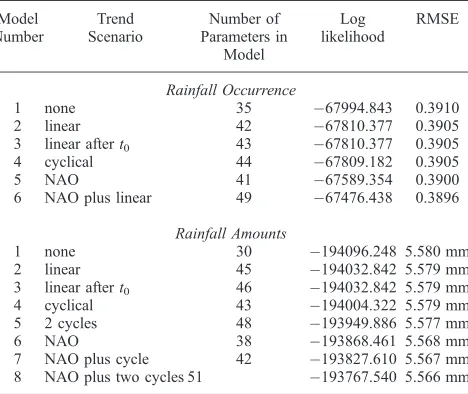
whereYiis the observed response for theith case, andmiand siare the modeled mean and standard deviation. If the fitted model is correct, all of the Pearson residuals have expectation zero and variance 1. In particular, the mean Pearson residual for any subset of the data should be close to zero, and the root mean squared residual should be close to 1. By appropriate selection of subsets, we can therefore use the residuals to check for unexplained structure. An example is given in Figure 3. The top plots here show the mean and root mean square of Pearson residuals in each year from occurrence model 5 in Table 1, which includes the NAO as a predictor. The dashed lines on the mean plot Table 1. Summary of Models for the Daily Rainfall Record in the
Galway Bay Areaa
Model Number
Trend Scenario
Number of Parameters in
Model
Log likelihood
RMSE
Rainfall Occurrence
1 none 35 67994.843 0.3910
2 linear 42 67810.377 0.3905
3 linear aftert0 43 67810.377 0.3905 4 cyclical 44 67809.182 0.3905
5 NAO 41 67589.354 0.3900
6 NAO plus linear 49 67476.438 0.3896
Rainfall Amounts
1 none 30 194096.248 5.580 mm
2 linear 45 194032.842 5.579 mm 3 linear aftert0 46 194032.842 5.579 mm 4 cyclical 43 194004.322 5.579 mm 5 2 cycles 48 193949.886 5.577 mm
6 NAO 38 193868.461 5.568 mm
7 NAO plus cycle 42 193827.610 5.567 mm 8 NAO plus two cycles 51 193767.540 5.566 mm
a
are approximate 95% confidence bands about zero; if the model is correct, around 95% of mean residuals should lie within these bands. The bands are adjusted for dependence between sites, as described byWheater et al.[2000, chap. 4]. Their increased width in 1941 and 1997 is due to incomplete records for these years (there are only 22 observations from 1941, and 342 from 1997; recall that on average there are 8.47 observations per day). It is clear from this plot that there is a systematic downward trend in mean residuals between 1940 and 1990. This motivated the addition of a linear trend, and its interactions, to obtain model 6. The annual residual structure for model 6 is shown in the bottom plots of Figure 3. The trend is no longer evident, and by and large the mean residuals lie within the confidence bands. Some lack of fit is evident in the 1950s, which may bear further investigation; apart from this, the only problem is an unusually large mean residual for 1994. No structure is apparent in the root mean square plots.
[37] Pearson residuals are also used to check that seasonal
structure is captured by the models (splitting the data set by month) and that regional effects are adequately represented (splitting by site). Seasonality is well represented by all of the models; site-by-site analyses reveal some problems, however. In occurrence model 6, for example, one third of the sites have mean residuals that differ from zero by more than 4 standard errors. However, there does not seem to be any organization in the mean residual pattern; it is therefore likely that the discrepancies here are due to gauge position-ing or observer practice, rather than to any deficiency in the model. For example, the mean residuals at sites G3 and G18 are0.0385 and 0.1559 respectively; the associated stand-ard errors are 0.0082 and 0.0239. Figure 1 shows that the two sites are almost identically located and that their periods
of record overlap. A closer examination of the data at these sites reveals that G3 has no trace values, but 17% of wet day values at G18 are traces. It is clear that trace days are being counted as dry at G3 but wet at G18: hence the model, in trying to fit to the average of the two sites, is overpredicting at G3 and underpredicting at G18. Similar explanations can be found for other apparent site-by-site discrepancies.
[38] As well as checking for systematic residual variation,
it is necessary to ensure that the probability structure of the fitted models is correct, since this is used to compute the likelihoods upon which inferences are based. For the amounts model, the simplest check is via quantile-quantile plots of residuals defined in such a way that, if the model is correct, all residuals have the same distribution. The meas-ure used here is the Anscombe residual which, for the gamma distribution, takes the form
rð ÞiA ¼ Yi
mi 1=3
: ð8Þ
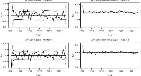
If the gamma assumption is correct, all Anscombe residuals have the same distribution which is approximately Gaus-sian; see, for example, Hougaard [1982]. A normal probability plot of Anscombe residuals can therefore be used to test this assumption. For amounts model 8, this plot is shown in Figure 4. The plot shows a good fit except in the lower tail of the distribution, where there are not as many small values as expected under a normal distribution. There are two reasons for this. The first is the presence of trace values, which account for almost all of the points in the lower tail and for which the exact rainfall amounts have been estimated as described in section 3.5 above. The second is that for highly skewed gamma distributions, the Figure 3. Annual structure of Pearson residuals from occurrence models 5 (incorporating NAO) and 6
Gaussian approximation breaks down in the lower tail since the normal distribution can yield negative values whereas the gamma cannot. To investigate the adequacy of the Gaussian approximation, the dashed line in Figure 4 shows the expected behavior if the gamma assumption is correct. This shows that a substantial part of the discrepancy can be attributed to a breakdown in the approximation. It also shows that the approximation is excellent elsewhere, and reveals some lack of fit in the upper tail of the distribution. However, this discrepancy is slight and there are few data points involved (around 0.6% of the sample), so that for the purposes of our analysis it is not a problem.
[39] For the occurrence model, we cannot use a
proba-bility plot to check the forecast probabilities. However, checks can be based on the idea that, if we collect together all of the days when the forecast probability of rain is close to some preassigned value p*, then the overall proportion of these days experiencing rain should be close to p*; see Dawid [1986]. For practical implementation, we collect together groups of days for which forecast probabilities are in the intervals (0.0, 0.1), (0.1, 0.2),. . ., (0.9, 1.0) and com-pute observed and expected proportions of rainy days within each of these groups (the expected proportion for a subset of Mcases with probabilities p1,. . .,pMisM1iM=1pi). Unless there is agreement within each forecast decile, there is something wrong with the probability structure of the model. The results, for occurrence model 6, are given in Table 2. This shows good agreement between observed and expected rain day proportions, throughout the range of the forecasts.
4.2. Model Interpretation
[40] Table 1 indicates that the best fitting models are
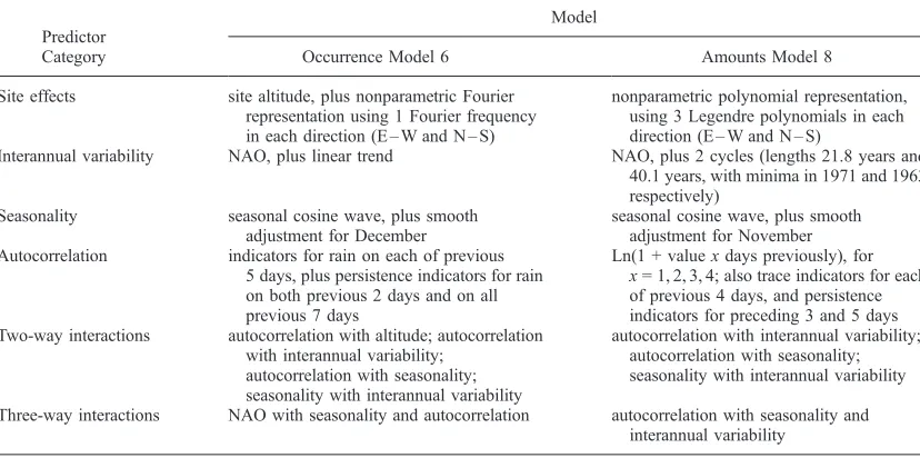
occurrence model 6 and amounts model 8. According to the checks above these both provide a good representation of the structure in the data, and their distributional assumptions are satisfied. The basic predictors in the two models are similar, and are summarized in Table 3. As well as describ-ing the predictors in the model, this shows the maximum likelihood estimates of the cycle lengths and phases for amounts model 8. The nominal standard errors for each of these parameters are small (the highest is 1.60, for the time at which the second cycle reaches its lowest point). The true standard errors will be larger however, as a result of spatial dependence which has not been accounted for here.
[41] Table 3 shows that both models contain a large
number of terms representing ‘‘autocorrelation’’ structure, particularly compared to other daily rainfall models in the literature (for example, Stern and Coe [1984] used just 1 previous day’s rainfall when modeling rainfall occurrence in West Africa); hence it may appear that our models are unnecessarily complex. However, the primary reason for including these terms is to ensure that within-sequence correlations do not affect inference regarding the effect of other variables upon rainfall. For this purpose it is better to include too many autocorrelation terms than too few. In any case, their inclusion is strongly supported by our analyses. For example, amounts model 8 contains a ‘‘persistence indicator’’ taking the value 1 at any site that has experienced rain on each of the previous 5 days, and zero otherwise. The effect of this indicator varies with the NAO and with the seasonal cycle so that, together with its interactions, it contributes 4 terms to the model. If these terms are dropped, the nominal log likelihood in Table 1 drops by 57.758. The correspondingp-value lies between 0.000 (under independ-ence) and 0.009 (under complete dependindepend-ence) so that such a reduction is unlikely to arise by chance.
[42] In each model, seasonal structure is represented by a
sine wave, with adjustments for individual months where necessary (i.e., for months with large mean Pearson resid-uals under a sine-wave-only model). The simplest adjust-ment is an indicator variable taking the value 1 during the appropriate month, and zero elsewhere. However, a referee has pointed out that this leads to an unnatural model since the resulting seasonal cycle contains discontinuities. We therefore use smooth adjustments based on scaled and shifted bisquare functions:
f dð Þ ¼ 1 2dð‘þ1ÞÞ
‘þ1
ð Þ
2
" #2
d¼1;. . .; ‘
ð Þ; ð9Þ
wheredis the day of the month and‘is the number of days in the month. These functions decay smoothly to zero at the Figure 4. Normal probability plot of Anscombe residuals
from amounts model 8. The dotted line shows the expected relationship if the gamma assumption is correct.
Table 2. Observed Versus Expected Proportions of Days With Rain, for Data Grouped According to Forecast Probability of Rainfall Occurrence (Occurrence Model 6)
Forecast Decile
1 2 3 4 5 6 7 8 9 10
ends of the month, with a maximum in the middle. The occurrence and amounts models contain adjustments for December and November respectively.
[43] To visualize the structure of the modeled site effects,
Figure 5 maps the surfaces defined by the Fourier and Legendre bases for each of the models. The effect of site altitude in the occurrence model is not included, so that in this case the map shows the regional structure after account-ing for altitude. Bearaccount-ing in mind that the fitted surfaces will be most reliable near gauges, both maps show physically meaningful structures. For the occurrence model the main features are a gentle west-east gradient, and an area of increased rainfall occurrence centered upon the end of Galway Bay. For the amounts model, the pattern is approx-imately constant except at the western margin, where there are enhanced intensities close to the sea from whence most weather systems arrive. The difference between the two
patterns suggests that the primary mechanisms controlling rainfall occurrence and amounts are different.
[44] It is of particular interest to try and interpret the
interactions in Table 3. Some are easily interpreted: for example, the interactions between seasonality and autocor-relation reflect the fact that temporal dependence in rainfall sequences is stronger in winter than in summer. This in turn has a physical interpretation in terms of the relative fre-quencies of convective and frontal weather systems: homo-geneous frontal systems account for a greater proportion of rainfall in winter than summer.
[45] The interactions of most interest, however, are those
involving the trend functions and the NAO, since these give detailed information about precisely how the rainfall pat-terns respond to interannual changes. For illustrative pur-poses, we consider the interaction between the NAO and seasonality in amounts model 8. For this model the
con-Figure 5. Spatial variation of rainfall as represented by (left) occurrence model 6 and (right) amounts model 8. For the occurrence model, contours represent contributions to the log odds at equation (2). For the amounts model, contours are multiplicative adjustments to a ‘‘baseline’’ level. Squares are locations of rain gauges (see Figure 1).
Table 3. Summary of Predictors in Best Fitting Occurrence and Amounts Models
Predictor Category
Model
Occurrence Model 6 Amounts Model 8
Site effects site altitude, plus nonparametric Fourier representation using 1 Fourier frequency in each direction (E – W and N – S)
nonparametric polynomial representation, using 3 Legendre polynomials in each direction (E – W and N – S)
Interannual variability NAO, plus linear trend NAO, plus 2 cycles (lengths 21.8 years and 40.1 years, with minima in 1971 and 1963 respectively)
Seasonality seasonal cosine wave, plus smooth adjustment for December
seasonal cosine wave, plus smooth adjustment for November Autocorrelation indicators for rain on each of previous
5 days, plus persistence indicators for rain on both previous 2 days and on all previous 7 days
Ln(1 + valuexdays previously), for x= 1, 2, 3, 4; also trace indicators for each of previous 4 days, and persistence indicators for preceding 3 and 5 days Two-way interactions autocorrelation with altitude; autocorrelation
with interannual variability; autocorrelation with seasonality; seasonality with interannual variability
autocorrelation with interannual variability; autocorrelation with seasonality; seasonality with interannual variability
tribution to the linear predictor (equation (3)), from terms involving just seasonal effects and the NAO, is
0:0611 cos2pday
365 0:2047 sin
2pday
365 0:0854fNOVðdayÞ
þð0:0419NAOÞ þ 0:0574NAOcos2pday 365
0:0112NAOsin2pday 365
; ð10Þ
where day is the ‘‘day’’ of the year (running from 1 to 365), fNOVis an adjustment of the form (9) for November, and
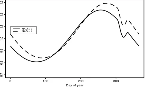
NAO is the current value of the monthly NAO index. [46] If we put NAO = 0 in (10), we obtain an ‘‘average’’
seasonal cycle; by putting NAO = 1 we obtain the corre-sponding cycle for a year in which NAO takes the value 1 in every month, i.e., in which there is a reasonably strong, and persistent, positive anomaly. (10) represents the contribution to the log mean rainfall: this corresponds to a multiplicative adjustment to the mean rainfall, which is plotted in Figure 6. According to Figure 6, rainfall amounts on wet days are highest, on average, in the autumn. The average effect of an enhanced NAO is to increase rainfall amounts substantially throughout the autumn and winter periods, with little effect in the summer. This agrees with our understanding of the NAO as a phenomenon whose effects are mainly confined to the Northern Hemisphere winter [Hurrell, 1995].
[47] Other interactions in the models can be studied in a
similar way. Broadly speaking, we find that the effects of the deterministic trends in each model are to induce wetter winters and drier summers. Moreover, the 3-way interac-tions involving the NAO suggest that, as well as increasing autumn and winter rainfall amounts, a positive anomaly is associated with decreased autocorrelation in winter rainfall sequences. A physical interpretation is that positive NAO anomalies are associated with weakened organisation in weather systems. The dynamics of this are unclear, but it may be linked to enhanced convective activity.
[48] Combining all of these results, we find that the
extended period of unusually high NAO values in the 1990s is undoubtedly responsible, to some extent, for the high winter rainfalls in our study area. The NAO does
not explain all of the trends in rainfall patterns, however: there are other changes, which we have approximated by linear and cyclical trend functions, that have also tended to increase winter rainfalls.
5. Summary and Conclusions
[49] In this work, we have attempted to demonstrate the
potential of GLMs for interpreting historical rainfall records. Because the daily data are so noisy, a more conventional approach may have focused on analyses of monthly data; however, it is unlikely that such an approach would have highlighted features such as the seasonally varying impact of the NAO upon the autocorrelation struc-ture of rainfall sequences. Despite the noise levels, the GLM methodology has detected a number of physically convinc-ing signals. The ability to model changconvinc-ing effects via interactions is an appealing feature, since it allows complex structures to be represented directly using relatively few parameters.
[50] It is often of particular interest to identify
associa-tions between large-scale climate indices, such as the NAO, and rainfall. For this type of problem, GLMs have the advantage over simpler methods (e.g., those based on correlations) that they implicitly allow us to account for other factors when testing for such associations. This is because inference is based on a comparison of likelihoods between a simple model (e.g., our occurrence model 1 and amounts model 1) and an extended model containing the effects of interest. The simple model effectively adjusts for all of the factors which it represents; the procedure therefore represents an elegant alternative to the common practice of standardization of all data prior to analysis, and allows us to work directly with the variable of interest rather than with anomalies.
[51] As well as illustrating how GLMs can be used to
model rainfall, we have demonstrated the use of simple but informative model checking techniques. In this study for example, residual analyses suggested that the NAO was not solely responsible for changes in rainfall patterns, and also highlighted a problem with the data at one of the sites; it is unlikely that this would have been spotted without the use of such techniques.
[52] In this paper, we have not exploited the idea that a
GLM is a probability model. For hydrological applica-tions, this is useful since it allows us to simulate daily rainfall sequences (this was one of the arguments for choosing to work with daily, rather than monthly, data). Many existing simulation techniques produce stationary sequences: a GLM is not restricted in this way, since GLM simulations will be conditioned upon the values of external predictors which may vary in both space and time. However, before using GLM simulations for hydro-logical applications it is necessary to carry out further checks. Our results indicate that systematic structure in day-to-day rainfall distributions has been captured; how-ever, it is possible that small errors in the models may be magnified when it comes to the reproduction of features of hydrological interest, such as extremes of areal average rainfall at monthly or longer timescales. Further details and some results indicating that the models are indeed able to reproduce such features are given by Wheater et al. [2000].
[53] There is one theoretical issue that has not been
addressed here: this is the effect of intersite dependence upon likelihood-based inference. This is the subject of ongoing research, both in our own work and in the wider statistical community. In particular, the generalized estimat-ing equation (GEE) approach introduced by Liang and Zeger [1986] is gaining in popularity. However, there is some evidence that the use of an incorrect dependence structure within a GEE approach can actually produce worse results than using an independence structure [ McDo-nald, 1993; Crowder, 1995; Sutradhar and Das, 1999]. Ultimately, any technique must be judged on the plausibility of the results it produces. In this paper, informal interpre-tation of nominal log likelihoods has been combined with careful residual analysis to guide the model-building proc-ess. The results (along with those from similar studies in the UK and elsewhere) are, we believe, convincing.
[54] Acknowledgments. This work was begun as part of a project funded by the Office of Public Works, Dublin, Ireland, and was subse-quently funded in part by the UK Ministry of Agriculture, Fisheries and Food. The involvement of Denis Peach (now at the British Geological Survey) in managing the former project is warmly acknowledged, as is that of Sally Watson. Data, and logistical support, were provided by Jennings O’Donovan and partners. We also thank the referees for their thoughtful and constructive comments on an earlier version of the paper. All of the model fitting reported here has been carried out using FORTRAN software, which is available via Internet from http://www.homepagesucl.ac.uk/ ucakarc/ work/glimclim.html.
References
Abramowitz, M., and I. A. Stegun,Handbook of Mathematical Functions: With Formulas, Graphs and Mathematical Tables, Dover, Mineola, N. Y., 1965.
Chandler, R. E., Model checking, inEncyclopedia of Biostatistics, edited by P. Armitage and T. Colton, pp. 2666 – 2668, John Wiley, New York, 1998a.
Chandler, R. E., Orthogonality, inEncyclopedia of Biostatistics, edited by P. Armitage and T. Colton, pp. 3203 – 3209, John Wiley, New York, 1998b.
Chandler, R. E. and H. S. Wheater, Climate change detection using general-ized linear models for rainfall—A case study from the west of Ireland, I, Preliminary analysis and modelling of rainfall occurrence,Tech. Report 194, Dep. of Stat. Sci., Univ. Coll. London, London, 1998a. (Available at http://www.ucl.ac.uk/Stats/research/abstracts.html).
Chandler, R. E., H. S. Wheater, Climate change detection using generalized linear models for rainfall—A case study from the west of Ireland, II, Modelling of rainfall amounts on wet days,Tech. Rep. 195, Dep. of Stat. Sci., Univ. Coll. London, London, 1998b. (Available at http://www.ucl. ac.uk/Stats/research/abstracts.html).
Coe, R., and R. D. Stern, Fitting models to daily rainfall,J. Appl. Meteorol., 21, 1024 – 1031, 1982.
Cox, D. R., and D. V. Hinkley,Theoretical Statistics, Chapman and Hall, New York, 1974.
Crowder, M., On the use of a working correlation matrix in using general-ised linear models for repeated measures,Biometrika,82(2), 407 – 410, 1995.
Daly, D., A report on the flooding in the Gort-Ardrahan area, report, Geo-logical Survey of Ireland, Dublin, 1992.
Dawid, A. P., Probability forecasting, in Encyclopedia of Statistical Sciences, edited by S. Kotz and N. Johnson, pp. 210 – 218, John Wiley, New York, 1986.
Dobson, A. J.,An Introduction to Generalized Linear Models, Chapman and Hall, New York, 1990.
Department of the Environment (DOE), UK Climate Change Impacts Re-view Group: ReRe-view of the potential effects of climate change in the UK, HMSO, London, 1996.
Fahrmeir, L., and G. Tutz, Multivariate Statistical Modelling Based on Generalized Linear Models, Springer-Verlag, New York, 1994. Green, P. J., Iteratively reweighted least squares for maximum likelihood
estimation, and some robust and resistant alternatives,J. R. Stat. Soc., Ser. B,46(2), 149 – 192, 1984.
Hougaard, P., Parametrizations of nonlinear models,J. R. Stat. Soc., Ser. B, 44, 244 – 252, 1982.
Hurrell, J. W., Decadal trends in the North Atlantic Oscillation: Regional temperatures and precipitation,Science,269, 676 – 679, 1995. Jones, P. D., T. Jo´nsson, and D. Wheeler, Extension to the North Atlantic
Oscillation using early instrumental pressure observations from Gibraltar and south-west Iceland,Int. J. Climatol.,17, 1433 – 1450, 1997. Liang, K.-Y., and S. L. Zeger, Longitudinal data analysis using generalized
linear models,Biometrika,73(1), 13 – 22, 1986.
McCullagh, P., and J. A. Nelder, Generalized Linear Models, 2nd ed., Chapman and Hall, New York, 1989.
McDonald, B. W., Estimating logistic regression parameters for bivariate binary data,J. R. Stat. Soc., Ser. B,55(2), 391 – 397, 1993.
Office of Public Works (OPW), An investigation of the flooding problems in the Gort-Ardrahan area of south Galway, by Southern Water Global and Jennings O’Donovan and partners, Dublin, 1998.
Pfister, C., Monthly temperature and precipitation in central Europe 1525 – 1979: quantifying documentary evidence on weather and its effects, in Climate Since A.D. 1500, edited by R. Bradley and P. Jones, pp. 118 – 142, Routledge, New York, 1992.
Priestley, M. B.,Spectral Analysis and Time Series, Academic, San Diego, Calif., 1981.
Stern, R. D., and R. Coe, A model fitting analysis of rainfall data (with discussion),J. R. Stat. Soc., Ser. A,147, 1 – 34, 1984.
Sutradhar, B. C., and K. Das, On the efficiency of regression estimators in generalised linear models for longitudinal data,Biometrika,86(2), 459 – 465, 1999.
Wei, B.-C.,Exponential Family Nonlinear Models,Lect. Notes Stat., 130, 1997.
Wheater, H. S., V. S. Isham, C. Onof, R. E. Chandler, P. J. Northrop, P. Guiblin, S. M. Bate, D. R. Cox, and D. Koutsoyiannis, Generation of spatially consistent rainfall data,Tech. Rep. 204, Dep. of Stat. Sci., Univ. Coll. London, London, 2000. (Available at http://www.ucl.ac.uk/Stats/ research/abstracts.html).