Towards a Visipedia: Combining Computer Vision and Communities of Experts

(1)

Communities of Experts

Thesis by

Grant Van Horn

In Partial Fulfillment of the Requirements for the

Degree of

Doctor of Philosophy

CALIFORNIA INSTITUTE OF TECHNOLOGY

Pasadena, California

2019

(2)

Grant Van Horn

ORCID: 0000-0003-2953-9651

(3)

ACKNOWLEDGEMENTS

First and foremost I would like to thank my parents, Mathew and Mary Van Horn.

I dedicate this work to them.

I would like to thank my advisor, Pietro Perona. I hope that at least a fraction of his

curiosity for the world has worn off on me. It has been a pleasure to be a Slacker in

his lab.

I would like to thank Serge Belongie, who I consider a joint advisor. I owe most

of my opportunities from the last decade to Serge, and owe my current path in life

to his guidance. I am forever grateful that he advised me during my undergraduate

career, my Masters, and my Ph.D.

I would like to thank Steve Branson, easily my most influential mentor. From Steve,

I learned how to identify problems, how to conduct research, and how to discuss

the findings. I owe a lot to him, and I am very proud of the work we accomplished

together.

I would like to thank Jessie Barry and the rest of her team at the Cornell Lab of

Ornithology. I would also like to thank Scott Loarie and the rest of the iNaturalist

team. I am grateful that I could work on both the Merlin and iNaturalist applications during my graduate studies, helping me connect my passion for computer science

with my passion for the outdoors.

Finally, I owe my most enjoyable moments at Caltech to the Vision Lab, and I would

like to thank all the Slackers I overlapped with: David Hall, Oisin Mac Aodha,

Matteo Ruggero Ronchi, Joe Marino, Ron Appel, Mason McGill, Sara Beery,

Alvita Tran, Natalie Bernat, Eyrun Eyjolfsdottir, Bo Chen, Krzysztof Chałupka,

Serim Ryou, Cristina Segalin, Eli Cole, Jennifer Sun, Jan Dirk Wegner, Daniel

(4)

ABSTRACT

Motivated by the idea of a Visipedia, where users can search and explore by image,

this thesis presents tools and techniques for empowering expert communities through

computer vision. The collective aim of this work is to provide a scalable foundation

upon which an application like Visipedia can be built. We conduct experiments using two highly motivated communities, the birding community and the naturalist

community, and report results and lessons on how to build the necessary components

of a Visipedia. First, we conduct experiments analyzing the behavior of

state-of-the-art computer vision classifiers on long tailed datasets. We find poor feature sharing

between classes, potentially limiting the applicability of these models and

empha-sizing the ability to intelligently direct data collection resources. Second, we devise

online crowdsourcing algorithms to make dataset collection for binary labels,

multi-class labels, keypoints, and mulit-instance bounding boxes faster, cheaper, and more

accurate. These methods jointly estimate labels, worker skills, and train computer vision models for these tasks. Experiments show that we can achieve significant cost

savings compared to traditional data collection techniques, and that we can produce

a more accurate dataset compared to traditional data collection techniques. Third,

we present two fine-grained datasets, detail how they were constructed, and analyze

the test accuracy of state-of-the-art methods. These datasets are then used to create

applications that help users identify species in their photographs: Merlin, an app

assisting users in identifying birds species, and iNaturalist, an app that assists users

in identifying a broad variety of species. Finally, we present work aimed at reducing

the computational burden of large scale classification with the goal of creating an application that allows users to classify tens of thousands of species in real time on

their mobile device. As a whole, the lessons learned and the techniques presented

(5)

PUBLISHED CONTENT AND CONTRIBUTIONS

Van Horn, Grant and Pietro Perona (2019). “Reducing Memory & Computation Demands for Large Scale Visual Classification”.

G.V.H. participated in designing the project, developing the method, running the experiments and writing the manuscript.

Van Horn, Grant, Steve Branson, Scott Loarie, et al. (2018). “Lean Multiclass Crowdsourcing”. In: Proceedings of the IEEE Conference on Computer Vision and Pattern Recognition. Salt Lake City, UT. doi:10.1109/cvpr.2018.00287. G.V.H. participated in designing the project, developing the method, running the experiments and writing the manuscript.

Van Horn, Grant, Oisin Mac Aodha, et al. (2018). “The iNaturalist Species Clas-sification and Detection Dataset”. In: Proceedings of the IEEE Conference on Computer Vision and Pattern Recognition. Salt Lake City, UT. doi:10.1109/ CVPR.2018.00914.

Branson, Steve, Grant Van Horn, and Pietro Perona (2017). “Lean Crowdsourcing: Combining Humans and Machines in an Online System”. In:Proceedings of the IEEE Conference on Computer Vision and Pattern Recognition, pp. 7474–7483. doi:10.1109/CVPR.2017.647.

Van Horn, Grant and Pietro Perona (2017). “The Devil is in the Tails: Fine-grained Classification in the Wild”. In: arXiv preprint arXiv:1709.01450. url:https: //arxiv.org/abs/1709.01450.

Van Horn, Grant, Steve Branson, Ryan Farrell, et al. (2015). “Building a bird recognition app and large scale dataset with citizen scientists: The fine print in fine-grained dataset collection”. In: Proceedings of the IEEE Conference on Computer Vision and Pattern Recognition, pp. 595–604. doi: 10.1109/CVPR. 2015.7298658.

(6)

INTRODUCTION

Visipedia, a community-generated visual encyclopedia, is the primary motivator and

inspiration for the work in this thesis. The Visipedia project1has been spearheaded

by Pietro Perona’s group at Caltech and Serge Belongie’s group, first at UCSD and

then Cornell Tech. This thesis is the most recent in a series of theses (Welinder,

2012; Branson, 2012; Wah, 2014), coming out of Perona and Belongie’s respective

groups, that attempts to make Visipedia a reality. In (Perona, 2010), Perona specifies the vision for Visipedia, defines the users and challenges of such a system, and muses

on its feasibility. He identifies two primary interfaces that Visipedia must provide.

First, Visipedia must provide an interface that allows users to ask visual questions.

Perona imagines an interface that can segment a photograph into its meaningful

component regions and then associates each of those regions with their

correspond-ing Wikipedia entry or to the same region in vast collections of photographs. This

would enable a user to photograph a rock pigeon and then click on the operculum

(i.e. the white, fleshy part at the base of the bill) to learn more about what purpose that structure serves. Similarly, this type of interface would enable a user to

nav-igate to the Wikipedia page for Amanita pantherinasimply from a photograph of

that fungus. Similar types of interactions could be had with photographs outside

the natural world: a photograph of a painting could be annotated with the artist’s

information; a photograph of a car engine could be annotated with the engine part

names and replacement information; a photograph of a retina could be annotated

with defects and linked to similar clinical cases.

To provide answers to the visual queries discussed in the previous paragraph,

Visi-pedia must first be made aware of the visual properties of the world and their

relationships. This is the second primary interaction with Visipedia: an interface

that allows experts to share their visual knowledge of the world. Perona imagines

an easy-to-use annotation interface that allows experts to contribute their visual

knowledge by annotating a few paradigmatic images. An ornithologist could

pro-vide information on bird morphology for a few different families. A mycologist

could provide example photographs of fungi species. A Chevrolet engineer could

(9)

provide engine part schematics. An ophthalmologist could provide example retina

images along with their prognosis. Perona emphasizes the importance of making this interface easy and quick, as experts’ time is scarce and valuable, and annotating

all of the important regions of an image is laborious and boring.

A high degree of automation is required to power the interactions that make these

two interfaces useful. A user, with a fleeting curiosity to identify the white, fleshy bit

of a pigeon, would prefer immediate results rather than waiting for a human expert

to answer. Similarly, an ornithologist would not annotate thousands of images

with the anatomical parts of a bird. Instead, we would prefer if machines could analyze images and immediately return results and efficiently propagate information

from tens of examples to thousands or millions of photographs. This introduces

two additional types of people that would interact with Visipedia: annotators and

machine vision researchers.

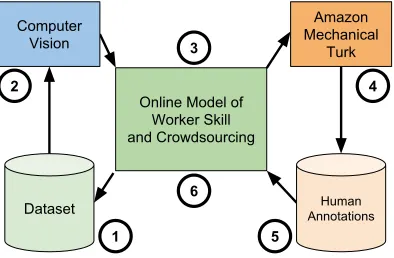
Annotators, or “eye balls for hire” (Perona, 2010), are the bridge connecting the

few samples provided by an expert to the thousands of examples required to train

modern computer vision models. Annotators could be paid crowd workers (e.g.

Amazon Mechanical Turk workers), they could be motivated enthusiasts (e.g. citizen scientists) or they could be people tasked with doing a few annotations while trying to

achieve another goal (e.g. GWAPs (Von Ahn and Dabbish, 2004) or Captchas (Von

Ahn, Maurer, et al., 2008)). In any case, their job is to propagate the expert

information to additional training data that can be used to train a computer vision

model to do the task. Machine vision researchers are responsible for designing and

implementing these computer vision models. These models are then responsible

for annotating an image with hyperlinks that allow users to answer visual questions

(i.e. clickable component regions), working with experts to efficiently incorporate

their visual knowledge, and propagating expert information to additional images (effectively annotating the images of the web).

At this point, we have defined Visipedia as a community-generated visual

encyclo-pedia that has interfaces to answer visual questions and that enable experts to share

their visual knowledge. Annotators help propagate expert knowledge to additional

images, producing datasets that can be used to train computer vision models designed

by machine vision researchers. These same models power the question-answering

interface and interact with experts to efficiently incorporate their knowledge. In

(10)

vision models at the time were not capable of performing at the level of accuracy

necessary to be useful, and that the field had not yet attempted to build such com-plex, heterogeneous systems. In addition, he observed that self-diagnosing models

(capable of deciding when they should ask questions of humans), active incremental

learning (necessary for learning in the large scale, dynamic web environment), and

human-machine interaction were research topics largely ignored by the computer

vision research community, yet crucial for Visipedia. It has been 9 years since

Perona penned his vision, where do we stand now?

Powered by the return of convolutional neural networks (Krizhevsky, Sutskever, and

Hinton, 2012), hardware advancements and easy-to-use computational libraries

(Mar-tin Abadi et al., 2015), the computer vision field as a whole has made incredible progress during my graduate studies on the tasks of image classification (Krizhevsky,

Sutskever, and Hinton, 2012), object detection (Ren et al., 2017), keypoint

localiza-tion (Chen et al., 2018), and image segmentalocaliza-tion (He et al., 2017). Indeed, setting

aside the feasibility of collecting training data, the costs of training, and the size

of the resulting model, if a sufficiently large dataset can be collected for one the

previous tasks, then often the performance of the resulting convolutional neural

network model is adequate for production usage. Evidence of this progress can be

seen in the availability of computer vision-powered applications now available to

consumers. During my graduate career, I helped build two of these applications (iNaturalist and Merlin), available through the Google Play Store and and Apple

App Store, that help users identify species in their photographs. The iNaturalist

app2 has a server-based computer vision classifier that can help identify 25,000

species. The Merlin app3 has a computer vision classifier available directly on the

phone and can help users classify 2,000 bird species. Besides mobile applications,

perhaps the most impressive sign of progress is the availability of self-driving cars

(albeit limited in their scope for now) becoming available to consumers.

Computer vision has entered an era of big data, where the ability to collect larger

datasets – larger in terms of the number of classes, the number of images per class, and the level of annotation per image – appears to be paramount for continuing

performance improvement and expanding the set of solvable applications. However,

while the accuracy of computer vision models has seen a rapid improvement over the

last half-decade, our ability to collect datasets of sufficient size to train and evaluate

these models has remained essentially unchanged and presents a significant hurdle

(11)

to expanding the availability and utility of computer vision services. Indeed, the

title of this thesis is “Towards a Visipedia,” not “Visipedia: Mission Accomplished.” So in the interim period between (Perona, 2010) and this thesis, many of the key

challenges to actually building a Visipedia (namely the challenges associated with

annotating large datasets) were still largely ignored (excluding the contributions of

the previous theses on Visipedia). The work in this thesis, however, is aimed at

reducing the burden of collecting datasets and will hopefully lay the foundation for

building a Visipedia.

In (Perona, 2010), Perona suggested that a step towards integrating a Visipedia with

all of Wikipedia would be to focus on a well-defined domain with a community of highly motivated enthusiasts. This is precisely what we have done by

engag-ing with the birdengag-ing community through the Cornell Lab of Ornithology and the

naturalist community through iNaturalist. The following chapters, each of which

is self-contained, explore dataset properties, efficient methods of collection, and

training state-of-the-art methods for deploying classification services to these two

communities. In terms of building a broader Visipedia, the following chapters

con-tain useful information for interacting with different types of annotators, modeling

the skills of annotators and vision models, and how to reliably combine

informa-tion from multiple sources (both human and machine). Taken as whole, this thesis

is an attempt to fill in the missing pieces that provide the required automation to make Visipedia a reality. I will briefly summarize the chapters and the relevant

contributions.

In Chapter 1, we discuss the long tail property of real world datasets and the

effect this tail has on classification performance. Experiments show that

state-of-the-art methods do not share feature learning between classes and that new

training methodologies or collecting additional data in the tail is required to improve

performance.

In Chapter 2, we devise a method for online crowdsourcing of binary labels, key-points, and multi-instance bounding box annotations. This method is capable of

estimating worker skills and jointly trains computer vision models. We present

ex-periments that show significant cost savings and improvements in dataset accuracy

by using our model instead of traditional dataset collection techniques.

In Chapter 3, we extend our online crowdsourcing method to large-scale multiclass

annotations. Our method is capable of utilizing a taxonomy across the labels,

(12)

vision system. We present experiments that show significant accuracy gains over

traditional majority vote techniques.

In Chapter 4, we present the NABirds dataset, collected by the birding community

through the Cornell Lab of Ornithology. We present experiments comparing the

annotation performance of different groups of workers on different types of tasks.

We describe the benefit of tapping into a motivated community and how to best

harness its enthusiasm. We additionally present results on dataset noise and show

that modern state-of-the-art methods are resilient to a reasonable amount of noise.

In Chapter 5, we present the iNaturalist Species Classification and Detection Dataset,

collected by the naturalist community through iNaturalist. We describe dataset

col-lection and prepping methods and evaluate state-of-the art classifiers and detectors.

In addition, we conduct a competition to motivate the computer vision research

community to explore large-scale, fine-grained classification and detection.

In Chapter 6, we analyze multiple techniques for reducing the computational

bur-den of the final fully connected layer of traditional convolutional networks. We experiment with a novel taxonomic approach but find that a simple factorization and

training scheme allows us to reduce the amount of computation and memory by 25x

without any loss in accuracy.

Finally, in Chapter 7, I suggest directions for future work.

References

Branson, Steven (2012). “Interactive learning and prediction algorithms for com-puter vision applications”. PhD thesis. UC San Diego.

Chen, Yilun et al. (2018). “Cascaded pyramid network for multi-person pose esti-mation”. In:CVPR.

He, Kaiming et al. (2017). “Mask r-cnn”. In:Computer Vision (ICCV), 2017 IEEE International Conference on. IEEE, pp. 2980–2988.

Krizhevsky, Alex, Ilya Sutskever, and Geoffrey E Hinton (2012). “ImageNet Clas-sification with Deep Convolutional Neural Networks.” In:NIPS.

Martin Abadi et al. (2015). TensorFlow: Large-Scale Machine Learning on Het-erogeneous Systems. Software available from tensorflow.org. url: http : / / tensorflow.org/.

(13)

Ren, Shaoqing et al. (2017). “Faster r-cnn: Towards real-time object detection with region proposal networks”. In:PAMI.

Von Ahn, Luis and Laura Dabbish (2004). “Labeling images with a computer game”. In:Proceedings of the SIGCHI conference on Human factors in computing systems. ACM, pp. 319–326.

Von Ahn, Luis, Benjamin Maurer, et al. (2008). “recaptcha: Human-based character recognition via web security measures”. In:Science321.5895, pp. 1465–1468.

Wah, Catherine Lih-Lian (2014). “Leveraging Human Perception and Computer Vi-sion Algorithms for Interactive Fine-Grained Visual Categorization”. PhD thesis. UC San Diego.

(14)

C h a p t e r 2

THE DEVIL IS IN THE TAILS: FINE-GRAINED

CLASSIFICATION IN THE WILD

Van Horn, Grant and Pietro Perona (2017). “The Devil is in the Tails: Fine-grained Classification in the Wild”. In: arXiv preprint arXiv:1709.01450. url:https: //arxiv.org/abs/1709.01450.

2.1 Abstract

The world is long-tailed. What does this mean for computer vision and visual

recog-nition? The main two implications are: (1) the number of categories we need to consider in applications can be very large, and (2) the number of training examples

for most categories can be very small. Current visual recognition algorithms have

achieved excellent classification accuracy. However, they require many training

examples to reach peak performance, which suggests that long-tailed distributions

will not be dealt with well. We analyze this question in the context of eBird, a large

fine-grained classification dataset and a state-of-the-art deep network classification

algorithm. We find that: (a) peak classification performance on well-represented

categories is excellent, (b) given enough data, classification performance suffers

only minimally from an increase in the number of classes, (c) classification perfor-mance decays precipitously as the number of training examples decreases, and (d)

surprisingly, transfer learning is virtually absent in current methods. Our findings

suggest that our community should come to grips with the question of long tails.

2.2 Introduction

During the past five years we have witnessed dramatic improvement in the

per-formance of visual recognition algorithms (Russakovsky et al., 2015). Human

performance has been approached or achieved in many instances. Three concurrent

developments have enabled such progress: (a) the invention of ‘deep network’

algo-rithms where visual computation is learned from the data rather than hand-crafted by

experts (Fukushima and Miyake, 1982; LeCun et al., 1989; Krizhevsky, Sutskever,

and Hinton, 2012), (b) the design and construction of large and well-annotated datasets (Fei-Fei, Fergus, and Perona, 2004; Everingham and al., 2005; Deng et al.,

(15)

(a) (b) (c)

Figure 2.1: (a) The world is long-tailed. Class frequency statistics in real world datasets (birds, a wide array of natural species, and trees). These are long-tailed distributions where a few classes have many examples and most classes have few. (b)

The 4 experimental long tail datasets used in this work. We modeled the eBird dataset (blue curve in(a)) and created four long tail datasets by shifting the modeled eBird dataset down (fewer images) and to the left (fewer species) by different amounts. Classes are split into head and tail groups; images per class in the respective groups decay exponentially. (c)Approximation of a long tail dataset. This approximation allows us to more easily study the effects of head classes on tail class performance.

data to train learning-based algorithms, and (c) the availability of inexpensive and

ever more powerful computers, such as GPUs (Lindholm et al., 2008), for algorithm

training.

Large annotated datasets yield two additional benefits, besides supplying deep nets

with sufficient training fodder. The first is offering common performance

bench-marks that allow researchers to compare results and quickly evolve the best

algo-rithmic architectures. The second, more subtle but no less important, is providing researchers with a compass – a definition of the visual tasks that one ought to try

and solve. Each new dataset pushes us a bit further towards solving real world

challenges. We wish to focus here on the latter aspect.

One goal of visual recognition is to enable machines to recognize objects in the

world. What does the world look like? In order to better understand the nature

of visual categorization in the wild we examined three real-world datasets: bird

species, as photographed worldwide by birders who are members of eBird (Sullivan et al., 2009); tree species, as observed along the streets of Pasadena (Wegner

et al., 2016); and plants and animal species, as photographed by the iNaturalist

(www.inaturalist.org) community. One salient aspect of these datasets is that some

species are very frequent, while most species are represented by only few specimens

(Fig 2.1a). In a nutshell: the world is long-tailed, as previously noted in the

(16)

2011; Zhu, Anguelov, and Ramanan, 2014). This is in stark contrast with current

datasets for visual classification, where specimen distribution per category is almost uniformly distributed (see (Tsung-Yi Lin et al., 2014) Figure 5(a)).

With this observation in mind, we ask whether current state-of-the-art classification

algorithms, whose development is motivated and benchmarked by uniformly

dis-tributed datasets, deal well with the world’s long tails. Humans appear to be able to

generalize from few examples; can our algorithms do the same? Our experiments

show that the answer isno. While, when data is abundant, machine-vision

classifi-cation performance can currently rival humans, we find that this is emphatically not the case when data is scarce for most classes, even if a few are abundant.

This work is organized as follows: In Section 2.3, we review the related work. We

then describe the datasets and training process in Section 2.4, followed by an analysis

of the experiments in Section 2.5. We summarize and conclude in Section 2.6.

2.3 Related Work

Fine-Grained Visual Classification – The vision community has released many

fine-grained datasets covering several domains such as birds (Welinder et al., 2010;

Wah et al., 2011; Berg, Liu, et al., 2014; Van Horn et al., 2015), dogs (Khosla

et al., 2011; Liu et al., 2012), airplanes (Maji et al., 2013; Vedaldi et al., 2014), flowers (Nilsback and Zisserman, 2006), leaves (Kumar et al., 2012), trees (Wegner

et al., 2016) and cars (Krause, Stark, et al., 2013; Y.-L. Lin et al., 2014). These

datasets were constructed to be uniform, or to contain "enough" data for the task.

The recent Pasadena Trees dataset (Wegner et al., 2016) is the exception. Most

fine-grained research papers present a novel model for classification (Xu et al., 2015;

Tsung-Yu Lin, RoyChowdhury, and Maji, 2015; Farrell et al., 2011; Krause, Jin,

et al., 2015; Xie et al., 2015; Branson et al., 2014; Gavves et al., 2015; Simon

and Rodner, 2015; Göring et al., 2014; Shih et al., 2015; N. Zhang et al., 2014;

Berg and Belhumeur, 2013; Chai, Lempitsky, and Zisserman, 2013; Xiao et al.,

2015; Y. Zhang et al., 2016; Pu et al., 2014). While these methods often achieve state-of-the-art performance at the time of being published, it is often the case

that the next generation of convolutional networks can attain the same level of

performance without any custom modifications. In this work, we use the

Inception-v3 model (Szegedy et al., 2016), pretrained on ImageNet for our experiments. Some

of the recent fine-grained papers have investigated augmenting the original datasets

(17)

Xie et al., 2015; Van Horn et al., 2015). Krause et al. (Krause, Sapp, et al., 2016)

investigated the collection and use of a large, noisy dataset for the task of fine-grained classification and found that off the shelf CNN models can readily take advantage of

these datasets to increase accuracy and reach state-of-the-art performance. Krause

et al.mention, but do not investigate, the role of the long tail distribution of training

images. In this work, we specifically investigate the effect of this long tail on the

model performance.

Imbalanced Datasets – Techniques to handle imbalanced datasets are typically

split into two regimes: algorithmic solutions and data solutions. In the first regime, cost-sensitive learning (Elkan, 2001) is employed to force the model to adjust its

decision boundaries by incurring a non-uniform cost per misclassification; see (H.

He and Garcia, 2009) for a review of the techniques. The second regime concerns

data augmentation, achieved either through over-sampling the minority classes,

un-der sampling the majority classes, or synthetically generating new examples for the

minority classes. When using mini batch gradient descent (as we do in the

experi-ments), oversampling the minority classes is similar to weighting these classes more

than the majority classes, as in cost-sensitive learning. We conduct experiments on

over-sampling the minority classes. We also employ affine (Krizhevsky, Sutskever,

and Hinton, 2012) and photometric (Howard, 2013) transformations to synthetically boost the number of training examples.

Transfer Learning – Transfer learning (Pan and Yang, 2010) attempts to adapt

the representations learned in one domain to another. In the era of deep networks,

the simplest form of transfer learning is using features extracted from pretrained

ImageNet (Russakovsky et al., 2015) or Places (Zhou et al., 2014) networks, see

(Sharif Razavian et al., 2014; Donahue et al., 2014). The next step is actually

fine-tuning (Girshick et al., 2014) these pretrained networks for the target task (Yosinski et al., 2014; Agrawal, Girshick, and Malik, 2014; Oquab et al., 2014; Huh, Agrawal,

and Efros, 2016). This has become the standard method for obtaining baseline

numbers on a new target dataset and often leads to impressive results (Azizpour et

al., 2015), especially when the target dataset has sufficient training examples. More

sophisticated transfer learning methods (Long et al., 2015; Tzeng et al., 2015) are

aimed at solving the domain adaptation problem. In this work, we are specifically

interested in a single domain, which happens to contain a long tail distribution of

training data for each class. We investigate whether there is a transfer of knowledge

(18)

Low Shot Learning – We experiment with a minimum of 10 training images

per class, which falls into the realm of low shot learning, a field concerned with learning novel concepts from few examples. In (Wang and Hebert, 2016b), Wang

and Herbet learn a regression function from classifiers trained on small datasets to

classifiers trained on large datasets, using a fixed feature representation. Our setup

is different in that we want to allow our feature representation to adapt to the target

dataset, and we want a model that can classify both the well represented classes

and the sparsely represented classes. The recent work of Hariharan and Girshick in

(Hariharan and Girshick, n.d.) explored this setup specifically, albeit in the broad

domain of ImageNet. The authors propose a low shot learning benchmark and

implement a loss function and feature synthesis scheme to boost performance on under represented classes. However, their results showed marginal improvement

when using a high capacity model (at 10 images per class the ResNet-50 (K. He

et al., 2016) model performed nearly as well as their proposed method). Our

work aims to study the relationship between the well represented classes and the

sparse classes, within a single domain. Metric learning tackles the low-shot learning

problem by learning a representation space where distance corresponds to similarity.

While these techniques appear promising and provide benefits beyond classification,

they do not hold up well against simple baseline networks for the specific task of

classification (Rippel et al., 2015).

2.4 Experiment Setup

Datasets

We consider three different types of datasets: uniform, long tail, and approximate

long tail. We used images from eBird (ebird.org) to construct each of these datasets.

These images are real world observations of birds captured by citizen scientists and

curated by regional experts. Each dataset consists of a training, validation, and test split. When placing images into each split, we ensure that a photographer’s images

do not end up in multiple splits for a single species. The test set is constructed

to contain as many different photographers as possible (e.g. 30 images from 30

different photographers). The validation set is similarly constructed, and the train

set is constructed from the remaining photographers.

Uniform Datasets– The uniform datasets allow us to study the performance of the

classification model under optimal image distribution conditions. These datasets

(19)

dataset with 1K classes containing 1K or 10K images each due to a lack of data

from eBird. Each smaller dataset is completely contained within the larger dataset (e.g. the 10 class datasets are contained within the 100 class datasets, etc.). The test

and validation sets are uniform, with 30 and 10 images for each class respectively,

and remain fixed for a class across all uniform datasets.

Approx. Long Tail Datasets– To conveniently explore the effect of moving from a

uniform dataset to a long tail dataset we constructed approximate long tail datasets,

see Figure 2.1c. These datasets consist of 1K classes split into two groups: the

head classes and the tail classes. All classes within a group have the same number of images. We study two different sized splits: a 10 head, 990 tail split and a 100

head, 900 tail split. The 10 head split can have 10, 100, 1K, or 10K images in each

head class. The 100 head split can have 10, 100, or 1K images in each head class.

The tail classes from both splits can have 10 or 100 images. We use the validation

and test sets from the 1K class uniform dataset for all of the approximate long tail

datasets. This allows us to compare the performance characteristics of the different

datasets in a reliable way, and we can use the 1K class uniform datasets as reference

points.

Long Tail Datasets – The full eBird dataset, with nearly 3 million images, is not

amenable to easy experimentation. Rather than training on the full dataset, we

would prefer to model the image distribution and use it to construct smaller, tunable

datasets, see Figure 2.1b. We did this by fitting a two-piece broken power law to the

eBird image distribution. Each class,i ∈ [1,N], is put into the head group ifi <= h, otherwise it is put into the tail group, where his the number of head classes. Each

head class i contains y ·ia1 _{images, where} _y _{is the number of images in the most}

populous class anda1is the power law exponent for the head classes. Each tail class

ihasy·h(a1−a2)_·_ia2_where_a

2is the power law exponent for the tail classes. We used

linear regression to determine thata1 = −0.3472 anda2 = −1.7135. We fixed the

minimum number of images for a class to be 10. This leaves us with 2 parameters

that we can vary: y, which shifts the distribution up and down, andh which shifts

the distribution left and right. We analyze four long tail datasets by selectingyfrom

{1K, 10K} and h from {10, 100}. Each resulting dataset consists of a different

number of classes and therefore has a different test and validation split. We keep to

(20)

Model Training & Testing Details

Model– We use the Inception-v3 network (Szegedy et al., 2016), pretrained from

ILSVC 2012, as the starting point for all experiments. The Inception-v3 model

exhibits good trade-off between size of the model (27.1M parameters) and

classifi-cation accuracy on the ILSVC (78% top 1 accuracy) as compared to architectures

like AlexNet and VGG. We could have used the ResNet-50 model but opted for Inception-v3, as it is currently being used by the eBird development team.

Training – We have a fixed training regime for each dataset. We fine-tune the

pretrained Inception-v3 network (using TensorFlow (Martin Abadi et al., 2015)) by

training all layers using a batch size of 32. Unless noted otherwise, batches are

constructed by randomly sampling from the pool of all training images. The initial

learning rate is 0.0045 and is decayed exponentially by a factor or 0.94 every 4

epochs. Training augmentation consists of taking random crops from the image

whose area can range from 10% to 100% of the image, and whose aspect ratio can range from 0.7 to 1.33. The crop is randomly flipped and has random brightness

and saturation distortions applied.

Testing– We use the validation loss to stop the training by waiting for it to steadily

increase, signaling that the model is overfitting. We then consider all models up

to this stopping point and use the model with the highest validation accuracy for

testing. At test time, we take a center crop of the image, covering 87.5% of the

image area. We track top 1 image accuracy as the metric, as is typically used in

fine-grained classification benchmarks. Note that image accuracy is the same as class average accuracy for datasets with uniform validation and test sets, as is the

case for all of our experiments.

2.5 Experiments

Uniform Datasets

We first study the performance characteristics of the uniform datasets. We consider

two regimes: (1) we extract feature vectors from the pretrained network and train a linear SVM; and (2) we fine-tune the pretrained network, see Section 2.4 for the

training protocol. We use the activations of the layer before the final fully connected

layer as our features for the SVM and used the validation set to tune the penalty

parameter. Figure 2.2a plots the error achieved under these two different regimes.

We can see that fine-tuning the neural network is beneficial in all cases except the

(21)

(a) (b)

Figure 2.2: (a) Classification performance as a function of training set size on

uniform datasets. A neural network (solid lines) achieves excellent accuracy on

these uniform datasets. Performance keeps improving as the number of training examples increases to 10K per class – each 10x increase in dataset size is rewarded with a 2x cut in the error rate. We also see that the neural net scales extremely well with increased number of classes, increasing error only marginally when 10x more classes are used. Neural net performance is also compared with SVM (dashed lines) trained on extracted ImageNet features. We see that fine-tuning the neural network is beneficial in all cases except in the extreme case of 10 classes with 10 images each. (b) Example misclassifications. Four of the twelve images misclassified by the 10 class, 10K images per class model. Clockwise from top left: Osprey misclassified as Great Blue Heron, Bald Eagle (center of image) misclassified as Great Blue Heron, Cooper’s Hawk misclassified as Great Egret, and Ring-billed Gull misclassified as Great Egret.

quickly, even with extensive hyperparameter sweeps). The neural network scales

incredibly well with increasing number of classes, incurring a small increase in

error for 10x increase in the number of classes. This should be expected given that

the network was designed for 1000-way ImageNet classification. At 10k images per

class, the network is achieving 96% accuracy on 10 bird species, showing that the

network can achieve high performance given enough data. For the network, a 10x increase in data corresponds to at least a 2x error reduction. Keep in mind that the

opposite is true as well: as we remove 10x images, the error rate increases by at

least 2x. These uniform dataset results will be used as reference points for the long

tail experiments.

Uniform vs. Natural Sampling

The long tail datasets present an interesting question when it comes to creating the

(22)

(a) (b) (c)

Figure 2.3: Uniform vs. Natural Sampling – effect on error. Error plots for models trained with uniform sampling and natural sampling. (a)The overall error of both methods is roughly equivalent, with natural sampling tending to be as good or better than uniform sampling. (b) Head classes clearly benefit from natural sampling. (c)Tail classes tend to have the same error under both sampling regimes.

uniformly from all classes, or such that they are sampled from the natural distribution

of images? Uniformly sampling from the classes will result in a given tail image

appearing more frequently in the training batches than a given head image, i.e., we are oversampling the tail classes. To answer this question, we trained a model

for each of our approximate long tail datasets using both sampling methods and

compared the results. Figure 2.3 plots the error achieved with the different sampling

techniques on three different splits of the classes (all classes, the head classes, and the

tail classes). We see that both sampling methods often converge to the same error,

but the model trained with natural sampling is typically as good as or better than

the model trained with uniform sampling. Figure 2.4 visualizes the performance of

the classes under the two different sampling techniques for two different long tail

datasets. These figures highlight that the head classes clearly benefit from natural sampling, and the center of mass of the tail classes is skewed slightly towards the

natural sampling. The results for the long tail dataset experiments in the following

sections use natural sampling.

Transferring Knowledge from the Head to the Tail

Section 2.5 showed that the Inception-v3 architecture does extremely well on uniform

datasets, achieving 96% accuracy on the 10 class, 10K images per class dataset;

87.3% accuracy on the 100 class, 1K images per class dataset; and 71.5% accuracy

on the 1K class, 100 images per class dataset. The question we seek to answer

is: how is performance affected when we move to a long tail dataset? Figure 2.5a

summarizes our findings for the approximate long tail datasets (see Table 2.1 and

(23)

(a) (b)

Figure 2.4: Uniform vs. Natural Sampling – effect on accuracy. We compare the effect of uniformly sampling from classes vs. sampling from their natural image distribution when creating training batches for long tailed datasets, Section 2.5. We use 30 test images per class, so correct classification rate is binned into 31 bins. It is clear that the head classes (marked as stars) benefit from the natural sampling in both datasets. The tail classes in(a)have an average accuracy of 32.1% and 34.2% for uniform and natural sampling respectively. The tail classes in (b)have an average accuracy of 33.5% and 38.6% for uniform and natural sampling respectively. For both plots, head classes have 1000 images and tail classes have 10 images.

and 10 images in each class, the top 1 accuracy across all classes is 33.2% (this is

the bottom, leftmost blue point in the figure). If we designate 10 of the classes as

head classes, and 990 classes as tail classes, what happens when we increase the

number of available training data in the head classes (traversing the bottom blue

line in Figure 2.5a)? We see that the head class accuracy approaches the peak 10

class performance of 96% accuracy (reaching 94.7%), while the tail classes have

remained near their initial performance of 33.2%.

We see a similar phenomenon even if we are more optimistic regarding the number

of available training images in the tail classes, using 100 rather than 10 (the top

blue line in Figure 2.5a). The starting accuracy across all 1000 classes, each with

100 training images, is 71.5%. As additional images are added to the head classes,

the accuracy on the head classes again approaches the peak 10 class performance

(reaching 94%) while the tail classes are stuck at 71%.

We can be optimistic in another way by moving more classes into the head, therefore

making the tail smaller. We now specify 100 classes to be in the head, leaving 900

classes for the tail (the green points in 2.5a). We see a similar phenomenon even

in this case, although we do see a slight improvement for the tail classes when the

(24)

(a) (b)

Figure 2.5: Transfer between head and tail in approximate long tail datasets.

(a) Head class accuracy is plotted against tail class accuracy as we vary the number of training examples in the head and in the tail for the approximate long tail datasets. Each point is associated with its nearest label. The labels indicate (in base 10) how much training data was in each head class (H) and each tail class (T). Lines between points indicate an increase in either images per head class, or images per tail class. As we increase images in the head class by factors of 10, the performance on the tail classes remains approximately constant. This means that there is a very poor transfer of knowledge from the head classes to the tail classes. As we increase the images per tail class, we see a slight loss in performance in the head classes. The overall accuracy of the model is vastly improved though. (b) Histogram of error

rates for a long tail dataset. The same story applies here: the tail classes do not

benefit from the head classes. The overall error of the joint head and tail model is 48.6%. See Figure 2.6 for additional details.

little to no transfer learning occurring within the network. Only the classes that receive additional training data actually see an improvement in performance, even

though all classes come from the same domain. To put it plainly, an additional 10K

bird images covering 10 bird species does nothing to help the network learn a better

representation for the remaining bird species.

To confirm the results on the approximate long tail datasets, we experimented on

four long tail distributions modeled after the actual eBird dataset, see Section 2.4 for

details on the datasets. For these experiments, we trained three separate models, one

trained with all classes and the other two trained with the head classes or tail classes respectively. Figures 2.5b and 2.6 show the results. We see the same recurring story:

the tail performance is not affected by the head classes. Training a model solely

on the tail classes is as good as, or even better, than training jointly with the head

classes, even though the head classes are from the same domain and are doubling

(25)

(a) (b) (c)

Figure 2.6: Histogram of Error Rates for Long Tail Datasets. These plots com-pare the performance of the head and tail classes trained jointly (labeled Head and Tail respectively) vs. individually (labeled Head Only and Tail Only respectively). The dashed histograms represent the error rates for individual models (trained ex-clusively on the head (red) or tail (blue) classes), and the solid histograms represent the error rates of the head and tail classes within the joint model. The vertical lines mark the mean error rates. We see that the tail classes do not benefit from being trained with the head classes: the mean error rate of a model trained exclusively on the tail classes does as good or better than a model trained with both head and tail classes. The overall joint error of the models (dominated by the tail performance) are: 45.1% for (a), 47.1% for (b) and 49.2% for (c).

head classes to the tail classes. See Table 2.3 for the detailed results.

Dataset Images /

Head Class

Images / Tail Class

Overall ACC

Head ACC

Tail ACC

10 head classes 990 tail classes

100 100 71.5 55.7 71.6

100 10 33.7 61.3 33.4

1,000 10 34.8 89.3 34.2

10,000 10 35.4 94.7 34.8

100 head classes 900 tail classes

100 100 71.5 65.2 72.2

100 10 37.9 68.9 34.5

1000 10 43.3 86.1 38.6

Table 2.1: Top 1 accuracy for head and tail classes when going from uniform to

approximate long tail image distribution. The uniform dataset performance is the

first row for the respective datasets; the subsequent rows are approximate long tail datasets. We see that the head classes benefit from the additional training images (Head ACC increases), but the tail classes benefit little, if at all (Tail ACC).

Increasing Performance on the Head Classes

The experiments in Section 2.5 showed that we should not expect the tail classes to

benefit from additional head class training data. While we would ultimately like to

have a model that performs well on the head and tail classes, for the time being we

(26)

Dataset Images / Head

Images / Tail

Overall ACC

Head ACC

Tail ACC

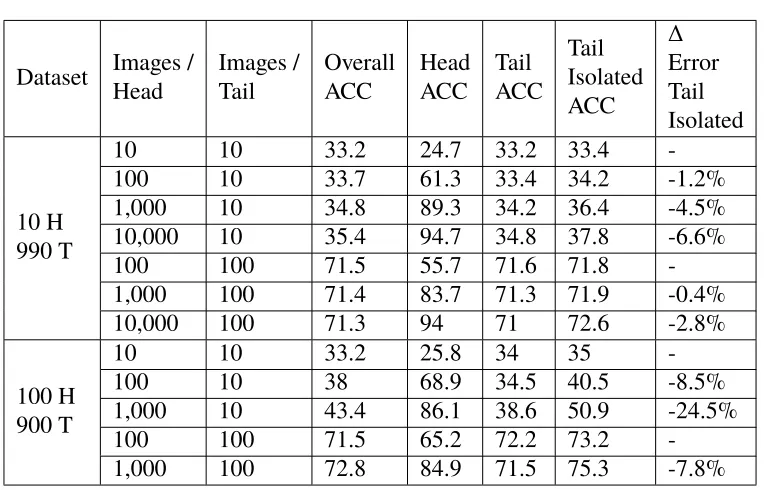
Tail Isolated ACC

∆

Error Tail Isolated

10 H 990 T

10 10 33.2 24.7 33.2 33.4

-100 10 33.7 61.3 33.4 34.2 -1.2%

1,000 10 34.8 89.3 34.2 36.4 -4.5%

10,000 10 35.4 94.7 34.8 37.8 -6.6%

100 100 71.5 55.7 71.6 71.8

-1,000 100 71.4 83.7 71.3 71.9 -0.4%

10,000 100 71.3 94 71 72.6 -2.8%

100 H 900 T

10 10 33.2 25.8 34 35

-100 10 38 68.9 34.5 40.5 -8.5%

1,000 10 43.4 86.1 38.6 50.9 -24.5%

100 100 71.5 65.2 72.2 73.2

-1,000 100 72.8 84.9 71.5 75.3 -7.8%

Table 2.2: Tail class performance. This table details the tail class performance in uniform and approximate long tail datasets. In addition to showing the accuracy of the tail classes (Tail ACC) we show the performance of tail classes in isolation from the head classes (Tail Isolated ACC). To compute Tail Isolated ACC, we remove all head class images from the test set and ignore the head classes when making predictions on tail class images. These numbers reflect the situation of using the head classes to improve the feature representation of the network. The∆Error Tail Isolated column shows the decrease in error between the tail performance when the head classes are considered (Tail ACC) and the tail performance in isolation (Tail Isolated ACC). These numbers are a sanity check to ensure that the tail classes do indeed benefit from a feature representation learned with the additional head class images. The problem is that the benefit of the representation is not shared when both the head and tail classes are considered together.

data, i.e. the head classes. In this section, we explore whether we can use the tail to

boost performance on the head classes. For each experiment, the model is trained

on all classes specified in the training regime (which may be the head classes only,

or could be the head and the tail classes), but at test time only head test images are

used and only the head class predictions are considered (e.g. a model trained for

1000 way classification will be restricted to make predictions for the 10 head classes

only).

We first analyze the performance of the head classes in a uniform dataset situation,

where we train jointly with tail classes that have the same number of training images

as the head classes. This can be considered the best case scenario for transfer

(27)

Dataset Params

Num Tail Classes

Overall ACC

Head ACC

Head Isolated ACC

Head Model ACC

Tail ACC

Tail Isolated ACC

Tail Model ACC h = 10

y = 1K 82 54.9 85.7 88.7 87.7 51.2 56.8 53

h = 10

y = 10K 343 52.9 89.7 94.3 92.6 51.8 53.6 52.1

h = 100

y = 1K 478 50.8 76.5 79.7 76.5 45.4 53.6 46.1

h = 100

y = 10K 2115 51.4 87.4 89.4 87 49.7 53.4 53

Table 2.3: Top 1 accuracy for the long tail datasets. This table details the results of the long tail experiments. See Section 2.4 for information on the dataset parameters. Three different models were trained for each dataset. 1. Whole ModelThis model was trained with both the head and the tail classes. Overall top 1 accuracy can be found in the Overall ACC column. Performance on the head and tail classes can be found in the Head ACC and Tail ACC columns respectively. Performance on the head and tail classes in isolation from each other can be found in the Head Isolated ACC and Tail Isolated ACC columns respectively. 2. Head ModelThis model was trained exclusively on the head classes. Overall top 1 accuracy (on the head classes only) can be found in the Head Model ACC column. 3. Tail ModelThis model was trained exclusively on the tail classes. Overall top 1 accuracy (on the tail classes only) can be found in the Tail Model ACC column.

are many more source classes than target classes. Figure 2.7a shows the results. In

both the 10 head class situation and 100 head class situation, we see drops in error

when jointly training the head and tail (dashed lines) as compared to the head only

model (solid lines).

The next experiments explore the benefit to the head in the approximate long tail

datasets. Figures 2.7b and 2.7c show the results. We found that there is a benefit to

training with the long tail, between 6.3% and 32.5% error reduction, see Table 2.4. The benefit of the tail typically decreases as the ratio of head images to tail images

increases. When this ratio exceeds 10, it is worse to use the tail during training.

In these experiments, we have been monitoring the performance of all classes during

training with a uniform validation set (10 images per class). This validation set is

our probe into the model, and we use it to select which iteration of the model to

use for testing. We now know that using as much tail data as possible is beneficial.

This raises the following question: can we monitor solely the head classes with the

(28)

be able to place all tail images in the training set rather than holding some out for

the validation set. The results shown in Figure 2.8 show that this is possible, and that it actually produces a more accurate model for the head classes.

Dataset Images / Head

Images / Tail

Head / Tail Image Ratio

Head Isolated ACC

Head Model ACC

∆

Error

10 H 990 T

10 10 0.01 66.6 55.6 -24.6%

100 10 0.1 77.3 74 -12.7%

1,000 10 1.01 91.3 88.6 -23.7%

10,000 10 10.1 94.6 96 +35%

100 100 0.01 85.6 74 -44.6%

1,000 100 0.1 92.3 88.6 -32.5%

10,000 100 1.01 96.3 96 -7.5%

100 H 900 T

10 10 0.11 49 40 -15%

100 10 1.11 74 70.2 -12.8%

1,000 10 11.11 86.8 87.3 +3.9%

100 100 0.11 81.6 70.2 -38.3%

1,000 100 1.11 88.1 87.3 -6.3%

Table 2.4: Head class performance. This table details the performance of the head classes under different training regimes. The Head Isolated ACC numbers show the top 1 accuracy on the head class images when using a model trained with both head and tail classes, but only makes predictions for the head classes at test time. The Head Model ACC numbers show the top 1 accuracy for a model that was trained exclusively on the head classes. We can see that it is beneficial to train with the tail classes until the head to tail image ratio exceeds 10, at which point it is better to train with the head classes only.

2.6 Discussion and Conclusions

The statistics of images in the real world are long-tailed: a few categories are highly

represented, and most categories are observed only rarely. This is in stark contrast with the statistics of popular benchmark datasets, such as ImageNet (Deng et al.,

2009), COCO (Tsung-Yi Lin et al., 2014), and CUB200 (Wah et al., 2011), where

the training images are evenly distributed amongst classes.

We experimentally explored the performance of a state-of-the-art classification

model on approximate and realistic long-tailed datasets. We make four observations which, we hope, will inform future research in visual classification.

First, performance is excellent, even in challenging tasks, when the number of

(29)

(a) (b) (c)

Figure 2.7: Head class performance when using additional tail categories. Head + Tail 10 refers to the tail having 10 images per class; Head + Tail 100 refers to the tail having 100 images per class. At test time we ignore tail class predictions for models trained with extra tail classes. We see that training with additional tail classes (dashed lines) decreases the error compared to a model trained exclusively on the head classes (solid lines) in both uniform and long tail datasets. In the long tail setting, the benefit is larger when the ratio of head images to tail images is smaller. We found that if this ratio exceeds 10, then it is better to train the model with the head classes only (right most points in (b) and (c)).

error rate is about 4% in the eBird dataset when each species is trained with 104

images (see Figure 2.2a). This is in line with the performance observed on ImageNet

and COCO, where current algorithms can rival humans.

Second, if the number of training images is sufficient, classification performance

suffers only minimally from an increase in the number of classes (see Figure 2.2a).

This is indeed good news, as we estimate that there are tens of millions of object

categories that one might eventually attempt to classify simultaneously.

Third, the number of training images is critical: classification error more than

doubles every time we cut the number of training images by a factor of 10 (see Figure

2.2a). This is particularly important in a long-tailed regime since the tails contain

most of the categories and therefore dominate average classification performance.

For example: the largest long tail dataset from our experiments contains 550,692

images and yields an average classification error of 48.6% (see Figure 2.5b). If

the same 550,692 images were distributed uniformly amongst the 2215 classes, the

average error rate would be about 27% (see Fig. 2.2a). Another way to put it: collecting the eBird dataset took a few thousand motivated birders about 1 year.

Increasing its size to the point that its top 2000 species contained at least 104images

would take 100 years (see Figure 2.1a). This is a long time to wait for excellent

accuracy.

(30)

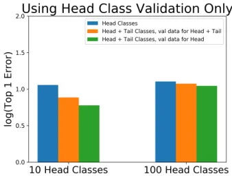
Figure 2.8: Using validation data from the head classes only. This plot shows the error achieved under different training regimes. Head Classes represents a model trained exclusively on the head classes, with 1000 training images each. The

Head + Tail Classes, val data for Head + Tail represents a model trained with

both head and tail classes (1000 images per head class, 100 images per tail class), and a validation set was used that had both head and tail class images. Head +

Tail Classes, val data for Headrepresents a model trained with both head and tail

classes (1000 images per head class, 100 images per tail class), and a validation set that only has head class images. We can see that it is beneficial to train with the extra tail classes, and that using the head classes exclusively in the validation set results in the best performing model.

current classification models. Simultaneously training on well-represented classes

does little or nothing for the performance on those classes that are least represented.

The average classification accuracy of the models will be dominated by the poor tail

performance, and adding data to the head classes will not improve the situation.

Our findings highlight the importance of continued research in transfer and low shot

learning (Fei-Fei, Fergus, and Perona, 2004; Hariharan and Girshick, n.d.; Wang and Hebert, 2016b; Wang and Hebert, 2016a) and provide baselines for future work

to compare against. When we train on uniformly distributed datasets, we sweep the

world’s long tails under the rug, and we do not make progress in addressing this

challenge. As a community, we need to face up to the long-tailed challenge and start

developing algorithms for image collections that mirror real-world statistics.

References

(31)

Azizpour, Hossein et al. (2015). “From generic to specific deep representations for visual recognition”. In:Proceedings of the IEEE Conference on Computer Vision and Pattern Recognition Workshops, pp. 36–45.

Berg, Thomas and Peter Belhumeur (2013). “POOF: Part-based one-vs.-one fea-tures for fine-grained categorization, face verification, and attribute estimation”. In:Proceedings of the IEEE Conference on Computer Vision and Pattern Recog-nition, pp. 955–962.

Berg, Thomas, Jiongxin Liu, et al. (2014). “Birdsnap: Large-scale fine-grained visual categorization of birds”. In:Computer Vision and Pattern Recognition (CVPR), 2014 IEEE Conference on. IEEE, pp. 2019–2026.

Branson, Steve et al. (2014). “Improved Bird Species Recognition Using Pose Nor-malized Deep Convolutional Nets.” In:BMVC. Vol. 1. 6, p. 7.

Chai, Yuning, Victor Lempitsky, and Andrew Zisserman (2013). “Symbiotic seg-mentation and part localization for fine-grained categorization”. In:Proceedings of the IEEE International Conference on Computer Vision, pp. 321–328.

Deng, Jia et al. (2009). “Imagenet: A large-scale hierarchical image database”. In:

Computer Vision and Pattern Recognition, 2009. CVPR 2009. IEEE Conference on. IEEE, pp. 248–255.

Donahue, Jeff et al. (2014). “DeCAF: A Deep Convolutional Activation Feature for Generic Visual Recognition.” In:Icml. Vol. 32, pp. 647–655.

Elkan, Charles (2001). “The foundations of cost-sensitive learning”. In: Interna-tional joint conference on artificial intelligence. Vol. 17. 1. LAWRENCE ERL-BAUM ASSOCIATES LTD, pp. 973–978.

Everingham, M. and et al. (2005). “The 2005 PASCAL Visual Object Classes Challenge”. In:First PASCAL Machine Learning Challenges Workshop, MLCW, pp. 117–176.

Farrell, Ryan et al. (2011). “Birdlets: Subordinate categorization using volumetric primitives and pose-normalized appearance”. In:Computer Vision (ICCV), 2011 IEEE International Conference on. IEEE, pp. 161–168.

Fei-Fei, Li, R. Fergus, and Pietro Perona (2004). “Learning Generative Visual Mod-els From Few Training Examples: An Incremental Bayesian Approach Tested on 101 Object Categories”. In:IEEE CVPR Workshop of Generative Model Based Vision (WGMBV).

Fukushima, Kunihiko and Sei Miyake (1982). “Neocognitron: A self-organizing neural network model for a mechanism of visual pattern recognition”. In: Com-petition and cooperation in neural nets. Springer, pp. 267–285.

(32)

Girshick, Ross et al. (2014). “Rich feature hierarchies for accurate object detection and semantic segmentation”. In:Proceedings of the IEEE conference on computer vision and pattern recognition, pp. 580–587.

Göring, Christoph et al. (2014). “Nonparametric part transfer for fine-grained recog-nition”. In:Computer Vision and Pattern Recognition (CVPR), 2014 IEEE Con-ference on. IEEE, pp. 2489–2496.

Hariharan, Bharath and Ross Girshick. “Low-shot Visual Recognition by Shrinking and Hallucinating Features”. In:

He, Haibo and Edwardo A Garcia (2009). “Learning from imbalanced data”. In:

Knowledge and Data Engineering, IEEE Transactions on21.9, pp. 1263–1284.

He, Kaiming et al. (2016). “Deep residual learning for image recognition”. In: Pro-ceedings of the IEEE Conference on Computer Vision and Pattern Recognition, pp. 770–778.

Howard, Andrew G (2013). “Some improvements on deep convolutional neural network based image classification”. In:arXiv preprint arXiv:1312.5402.

Huh, Minyoung, Pulkit Agrawal, and Alexei A Efros (2016). “What makes ImageNet good for transfer learning?” In:arXiv preprint arXiv:1608.08614.

Khosla, Aditya et al. (2011). “Novel Dataset for Fine-Grained Image Categoriza-tion”. In:First Workshop on Fine-Grained Visual Categorization, IEEE Confer-ence on Computer Vision and Pattern Recognition. Colorado Springs, CO.

Krause, Jonathan, Hailin Jin, et al. (2015). “Fine-grained recognition without part annotations”. In: Proceedings of the IEEE Conference on Computer Vision and Pattern Recognition, pp. 5546–5555.

Krause, Jonathan, Benjamin Sapp, et al. (2016). “The unreasonable effectiveness of noisy data for fine-grained recognition”. In:European Conference on Computer Vision. Springer, pp. 301–320.

Krause, Jonathan, Michael Stark, et al. (2013). “3d object representations for fine-grained categorization”. In: Proceedings of the IEEE International Conference on Computer Vision Workshops, pp. 554–561.

Krizhevsky, Alex, Ilya Sutskever, and Geoffrey E Hinton (2012). “ImageNet Clas-sification with Deep Convolutional Neural Networks.” In:NIPS.

Kumar, Neeraj et al. (2012). “Leafsnap: A computer vision system for automatic plant species identification”. In:Computer Vision–ECCV 2012. Springer, pp. 502–516.

LeCun, Yann et al. (1989). “Backpropagation applied to handwritten zip code recog-nition”. In:Neural computation1.4, pp. 541–551.

Lin, Tsung-Yi et al. (2014). “Microsoft COCO: Common objects in context”. In:

(33)

Lin, Tsung-Yu, Aruni RoyChowdhury, and Subhransu Maji (2015). “Bilinear CNN models for fine-grained visual recognition”. In:Proceedings of the IEEE Interna-tional Conference on Computer Vision, pp. 1449–1457.

Lin, Yen-Liang et al. (2014). “Jointly optimizing 3d model fitting and fine-grained classification”. In:Computer Vision–ECCV 2014. Springer, pp. 466–480.

Lindholm, Erik et al. (2008). “NVIDIA Tesla: A unified graphics and computing architecture”. In:IEEE micro28.2.

Liu, Jiongxin et al. (2012). “Dog breed classification using part localization”. In:

Computer Vision–ECCV 2012. Springer, pp. 172–185.

Long, Mingsheng et al. (2015). “Learning Transferable Features with Deep Adap-tation Networks.” In:ICML, pp. 97–105.

Maji, Subhransu et al. (2013). “Fine-grained visual classification of aircraft”. In:

arXiv preprint arXiv:1306.5151.

Martin Abadi et al. (2015). TensorFlow: Large-Scale Machine Learning on Het-erogeneous Systems. Software available from tensorflow.org. url: http : / / tensorflow.org/.

Nilsback, Maria-Elena and Andrew Zisserman (2006). “A visual vocabulary for flower classification”. In:Computer Vision and Pattern Recognition, 2006 IEEE Computer Society Conference on. Vol. 2. IEEE, pp. 1447–1454.

Oquab, Maxime et al. (2014). “Learning and transferring mid-level image repre-sentations using convolutional neural networks”. In: Proceedings of the IEEE conference on computer vision and pattern recognition, pp. 1717–1724.

Pan, Sinno Jialin and Qiang Yang (2010). “A survey on transfer learning”. In:IEEE Transactions on knowledge and data engineering22.10, pp. 1345–1359.

Pu, Jian et al. (2014). “Which looks like which: Exploring inter-class relationships in fine-grained visual categorization”. In:Computer Vision–ECCV 2014. Springer, pp. 425–440.

Rippel, Oren et al. (2015). “Metric learning with adaptive density discrimination”. In:ICLR.

Russakovsky, Olga et al. (2015). “Imagenet large scale visual recognition challenge”. In:International Journal of Computer Vision115.3, pp. 211–252.

Salakhutdinov, Ruslan, Antonio Torralba, and Josh Tenenbaum (2011). “Learning to share visual appearance for multiclass object detection”. In:Computer Vision and Pattern Recognition (CVPR), 2011 IEEE Conference on. IEEE, pp. 1481–1488.

(34)

Shih, Kevin J et al. (2015). “Part Localization using Multi-Proposal Consensus for Fine-Grained Categorization”. In:BMVC.

Simon, Marcel and Erik Rodner (2015). “Neural activation constellations: Unsuper-vised part model discovery with convolutional networks”. In:Proceedings of the IEEE International Conference on Computer Vision, pp. 1143–1151.

Sullivan, Brian L et al. (2009). “eBird: A citizen-based bird observation network in the biological sciences”. In:Biological Conservation142.10, pp. 2282–2292.

Szegedy, Christian et al. (2016). “Rethinking the inception architecture for computer vision”. In:Proceedings of the IEEE Conference on Computer Vision and Pattern Recognition, pp. 2818–2826.

Tzeng, Eric et al. (2015). “Simultaneous deep transfer across domains and tasks”. In:

Proceedings of the IEEE International Conference on Computer Vision, pp. 4068– 4076.

Van Horn, Grant et al. (2015). “Building a bird recognition app and large scale dataset with citizen scientists: The fine print in fine-grained dataset collection”. In:Proceedings of the IEEE Conference on Computer Vision and Pattern Recog-nition, pp. 595–604. doi:10.1109/CVPR.2015.7298658.

Vedaldi, Andrea et al. (2014). “Understanding objects in detail with fine-grained attributes”. In: Proceedings of the IEEE Conference on Computer Vision and Pattern Recognition, pp. 3622–3629.

Wah, Catherine et al. (2011). “The caltech-ucsd birds-200-2011 dataset”. In:

Wang, Yu-Xiong and Martial Hebert (2016a). “Learning from Small Sample Sets by Combining Unsupervised Meta-Training with CNNs”. In:Advances in Neural Information Processing Systems, pp. 244–252.

– (2016b). “Learning to learn: Model regression networks for easy small sample learning”. In:European Conference on Computer Vision. Springer, pp. 616–634.

Wegner, Jan D et al. (2016). “Cataloging public objects using aerial and street-level images-urban trees”. In:Proceedings of the IEEE Conference on Computer Vision and Pattern Recognition, pp. 6014–6023.

Welinder, Peter et al. (2010). “Caltech-UCSD birds 200”. In:

Xiao, Tianjun et al. (2015). “The application of two-level attention models in deep convolutional neural network for fine-grained image classification”. In: Pro-ceedings of the IEEE Conference on Computer Vision and Pattern Recognition, pp. 842–850.