Complexity Reduction In Multiple Input Multiple Output Algorithms

Complexity Reduction In Multiple

Input Multiple Output Algorithms

Leon Gor, BE (Hons 1)

Submitted in fulfillment of the requirements for the

degree of

Doctor of Philosophy

March 2007

_________________________________

Thesis supervisor Prof. Michael Faulkner

Centre for Telecommunications and Microelectronics

Victoria University, Footscray Park Campus

P.O. BOX 14428 MCMC

Melbourne 8001

Declaration

I hereby declare the contents of this thesis are the results of original research and have not

been submitted for a higher degree to any other university or institution. The research

work presented in this thesis is carried out by me and to the best of my knowledge does

not contain any previously published or written works by another person except where

due reference is made in the text.

Wireless communication devices are currently enjoying increasing popularity and widespread use. The constantly growing number of users, however, results in the shortage of the available spectrum. Various techniques have been proposed to increase the spectrum efficiency of wireless systems to solve the problem. Multiple Input Multiple Output (MIMO) is one solution that employs multiple antennas at the transmitter and receiver. The MIMO algorithms are usually highly complex and computationally intensive. This results in increased power consumption and reduced battery lifespan. This thesis investigates the complexity – performance trade-off of two MIMO algorithms.

function. Log-Polar receivers were found to be clipping insensitive for the given target Symbol Error Rate (SER) of 1*10-3. This makes Log-Polar receivers an obvious choice for the system designers.

The second part of the thesis (chapter 4) addresses the complexity problem associated with the QR decomposition algorithm, which is frequently used as a faster alternative to channel inversion in a MIMO scheme. Channel tracking can be employed with QR equalization in order to reduce the pilot overhead of a MIMO system in a non-stationary environment. QR decomposition is part of the QR equalization method and has to be performed in every instance that the channel estimate is obtained. The high rate of the QR decomposition, a computationally intensive technique, results in a high computational complexity per symbol. Some novel modifications are proposed to address this problem. Reducing the repetition rate of QR decompositions and tracking R (the upper triangular matrix) directly, while holding unitary matrix Q fixed, can significantly reduce complexity per symbol at the expense of some introduced error. Additional modification of the CORDIC algorithm (a square root- and division-free algorithm used to perform QR decomposition) results in more than 80% of computational complexity savings.

Foreword

The contents of this thesis are the results of original research and have not been submitted for a higher degree to any other university or institution. This thesis investigates the complexity issues of techniques that use the Multiple Input Multiple Output (MIMO) approach. Two major works are described in the thesis. Chapter 3 investigates the effect of clipping induced by the limited dynamic range of the receiver Analog to Digital Converter (ADC) on the Space Time Block (STBC system. The novelty of this work highlights how physical implementation issues affect the performance of the well-known and popular Alamouti STBC algorithm. The results of this work were published in two papers

• L. Gor and M. Faulkner, "Effect of Soft Limiting in the Transmit Diversity Schemes

Employing Space Time Block Coding," The fourth international conference on modelling and simulation, Melbourne, Australia, 2002

• L. Gor and M. Faulkner, "A/D clipping effects on STBC scheme in receivers employing

direct conversion structure," Electronics Letters vol. 40, pp. 352-354, 2004.

submitted for publications in

• L. Gor and M. Faulkner, "Power reduction through upper triangular matrix tracking

in QR detection MIMO receivers," Vehicular Technology Conference (VTC), 2006.

• L. Gor and M. Faulkner, "Channel tracking for MIMO receivers," Applicant:

Australian Telecommunications Research Centre (ATCRC), Patent number:

Acknowledgements

Contents

1

INTRODUCTION AND THESIS OUTLINE ... 1

2

BACKGROUND INFORMATION ... 3

2.1 Propagation Characteristics of a Radio Channel ... 3

2.1.1 Large-scale path loss ... 4

2.1.2 Small-scale variations... 5

2.2 Diversity... 8

2.2.1 Spatial diversity... 8

2.2.2 Polarisation diversity... 9

2.2.3 Time diversity ... 9

2.2.4 Frequency diversity ... 9

2.3 Concept of Information... 9

2.4 Channel Capacity ... 10

2.5 Multiple Input Multiple Output Systems ... 11

2.5.1 Capacity of the Multiple Input Multiple Output system... 11

2.5.2 Using MIMO capacity... 13

3

SIMULATION-BASED CLIPPING ANALYSIS IN ALAMOUTI SPACE

TIME BLOCK CODES... 16

3.1 Chapter Outline ... 16

3.2 Introduction ... 17

3.2.1 Communication system based on STBC coding ... 17

3.2.2 Receiver architectures ... 20

3.2.3 Signal conversion ... 23

3.3 Clipping in SISO systems... 24

3.4 Clipping in Alamouti STBC Coded System ... 28

3.4.1 Square clipping... 28

3.4.2 Circular clipping... 30

3.5 Simulations and Comparisons... 31

3.6 Conclusions ... 33

4

COMPLEXITY REDUCTION THROUGH UPPER TRIANGULAR

MATRIX TRACKING IN QR DETECTION MIMO RECEIVERS ... 35

4.1 Chapter Outline ... 35

4.2 Introduction ... 36

4.2.1 IEEE 802.11 TGn channel model... 36

4.2.2 Detection in MIMO... 39

4.2.3 Review of existing MIMO channel-tracking schemes ... 45

4.3 Using Upper Triangular Matrix Tracking to Reduce Complexity per Symbol in a Linear ZF MIMO System ... 53

4.3.1 System model ... 53

4.3.2 Evaluation of tracking schemes... 56

4.3.3 Saving power through QR decomposition repetition rate reduction ... 64

4.3.4 Threshold detection in a practical system... 68

4.3.5 CORDIC-based QR decomposition... 73

4.3.6 Simulation results... 82

4.4 Evaluation of the two proposed strategies with VBLAST-MMSE detection and comparison with RLS based DFE scheme... 86

4.4.1 Introduction ... 86

4.4.2 Evaluation of tracking schemes... 87

4.5 Conclusions ... 98

5

CONCLUSIONS... 100

List of Figures

Figure 1. Multipath effect... 5

Figure 2. MIMO system employing multiple antennas at the receiver and transmitter... 12

Figure 3. Space Time Coded MIMO system setup ... 14

Figure 4. Spatial Multiplexing system structure ... 15

Figure 5. Simplified setup for 2X1 communication system based on STBC coding... 17

Figure 6. STBC coded system implementation based on DC receiver structure ... 20

Figure 7. Block diagram of the Log-Polar receiver ... 21

Figure 8. ADC broken down into a sampler and quantiser... 23

Figure 9. A conceptual example of the square clipping of a QPSK modulated signal ... 25

Figure 10. Soft limiting operation of ADC in a DC receiver... 25

Figure 11. Magnitude clipping in a Log-Polar receiver employing QPSK modulation... 27

Figure 12. Soft limiting operation of the ADC in a Log-Polar receiver ... 27

Figure 13. Simulation block diagram... 31

Figure 14. Lowest clip/average levels for 10-3 target SER, square clipping... 31

Figure 15. Sensitivity of STBC coded and SISO schemes to AWGN at 10-3 target SER. ... 33

Figure 16. (a) Doppler spectrums used in 802.11n and Clarke's models (b) 40km/h moving object causes peak at 194 Hz. fc=5.25GHz... 38

Figure 17. BER comparison, 4X4 system with channel known at the receiver and QPSK modulation. ... 43

Figure 18. A generic frame structure consisting of a training preamble and D payload data symbols ... 45

Figure 20. Autocorrelation of the channel and channel inverse for SISO, 2X2 MIMO and 4X4

MIMO channels ... 49

Figure 21. MIMO-OFDM structure with QR detection and channel tracking, initial channel estimates are obtained during the training session... 53

Figure 22. General packet structure employed in wireless LANs... 54

Figure 23. Decision-directed tracking and QR decomposition for the channel-tracking case... 56

Figure 24. An example of the indexing, QRD performed every 3rd symbol... 57

Figure 25. Decision-directed tracking and QR decomposition for the upper triangular matrix-tracking scenario ... 58

Figure 26. LMS configuration for tracking the AR matrix... 60

Figure 27. Comparison of tracking performance, perfect channel estimation and hence perfect Q and R is assumed at the first symbol... 62

Figure 28. The system model used to evaluate the channel or upper triangular matrix-tracking schemes... 65

Figure 29. MSEvs. packet length comparison of various scenarios in the presence of AWGN and fd=6Hz ... 67

Figure 30. Threshold detector block diagram ... 71

Figure 31. MSE vs. packet length comparison using threshold detector ... 72

Figure 32. Using CORDIC to obtain upper triangular matrix R and unitary Q of a 2X2 complex matrix. ... 75

Figure 33. (a) Conventional CORDIC with three micro-rotations. The micro-rotation angle is approximately halved for each consecutive iteration (b) CORDIC becomes inefficient when the input angle is small... 78

Figure 34. Reducing number of rotations to one, by considering all possible micro-rotations at each iteration... 78

Figure 35. The number of microrotations vs y x (= tan

( )

Figure 36. Complexity savings of the AR tracking with modified CORDIC over the H tracking with the conventional CORDIC in 2X2 system... 84

Figure 38. Decision-directed tracking and SQRD for the upper triangular matrix-tracking

scenario ... 90

Figure 39. Complexity per symbol vs QR (order) update time... 93

Figure 40. BER comparison for the stationary channel ... 95

Figure 41. Channel MSE for AR and H tracking strategies, SNR=20dB, fdT=1*10-3... 96

List of Acronyms

Acronym Description First used in section ADC Analog to Digital Converter 3.2.1

AGC Automatic Gain Control 3.2.2.1

AWGN Additive White Gaussian Noise

2.4

DC Direct Conversion 3.2.1

DFE Decision Feedback Equalizer 4.2.3.2

FFF Feed Forward Filter 4.2.3.2

FBF Feed Back Filter 4.2.3.2

iid independent identically

distributed

2.5.1

ISI Inter Symbol Interference 2.1.2.3

MIMO Multiple Input Multiple Output

2.5.1

MMSE Minimum Mean Squared

Error

4.2.2.1

MLSD Maximum Likelihood

Sequence Detection

4.2.2

OFDM Orthogonal Frequency

Division Multiplexing

2.1.2.3

SER Symbol Error Rate 3.1

SIC Successive Interference

Cancellation

2.5.2.1 SISO Single Input Single Output 1 SNR Signal to Noise Ratio 2.2.1

SQRD 4.2.2.3

STBC Space Time Block Coding 1

STC Space Time Coding 2.5.2.1

STTC Space Time Trellis Coding 2.5.2.1

VBLAST 4.2.2.2

VGA Variable Gain Amplifier 3.2.2.1 WLAN Wireless Local Area Network 4.3.1

List of principal symbols

Symbol Description First used in section

___

p

L

Path loss 2.1.1

fdT Normalized Doppler

frequency

2.1.2.2

M Number of receive antennas 2.5.1

N Number of transmit antennas 2.5.1

2 ε

σ Quantization noise power 3.2.3

AR Nearly upper triangular

matrix

4.3

Bc Coherence Bandwidth 2.1.2.1

C Channel capacity 2.4

Cn x n n x n matrix total complexity

to perform QR decomposition

4.3.5.5

CR Complexity of CORDIC in

the rotational mode

4.3.5.5

CV Complexity of CORDIC in

the vectoring mode

4.3.5.5

D Dynamic range of Analog to Digital Converter

3.2.3

erH Channel error matrix 4.3.2.1 erR Upper triangular matrix error 4.3.2.2

fd Doppler frequency 2.1.2.2

H(X) Entropy of the distribution of random variable X

2.4

H The channel matrix 2.5.1

hi Complex channel element 3.2.1

Mx, My Mantissas of binary numbers

x and y

4.3.5.4

n Complex Additive White Gaussian noise sample/vector

Symbol Description First used in section q Quantization step size 3.2.3

Q Unitary matrix 4.3.1

qm CORDIC orthogonal matrix 4.3.5.1

r Received clipped signal element

3.3.1

R Upper triangular matrix 4.3.1 S Orthogonal coding matrix 3.2.1 s Transmitted symbol/vector 3.2.1

S(f) Doppler spectrum of 802.11n channel

4.2.1

Tc Coherence time 2.1.2.2

VF Full scale range of Analog to

Digital Converter

3.2.3

y Received signal/vector 3.2.1

α Scaling coefficient 3.3.1

T Possible transmitted signal

vector for ML detection

4.2.2

θ Constellation size 4.2.2

( )

ϑ ⋅ Hard decision operator 4.2.2.1

A Linear mapping 4.2.2.1

2

n

σ AWGN variance 4.2.2.1

P Symbol error covariance

matrix

4.2.2.1

H Extended channel matrix 4.4.1

CH Complexity of the

channel-tracking system

4.4.2.1

CR Complexity of the upper

triangular matrix-tracking system

1 Introduction and Thesis Outline

Wireless systems of the future must accommodate rich information content applications like high-speed Internet, live video streaming, online gaming, and so forth. The demand for these capabilities is constantly growing; in fact, according to [2] there will be 300,000 wireless hotspots by the end of 2009. Sophisticated algorithms based on Multiple Input Multiple Output (MIMO) techniques were developed to realise this great information capacity demand. These are usually highly complex, high processing power algorithms. Handheld, battery-operated devices are the primary targets of these new technologies. The increased power consumption will shorten battery life, hence the problem of reducing the processing power of these algorithms or their complexity is of paramount importance. This dissertation investigates the power and complexity issues of some of these algorithms.

Alamouti Space Time Block (STBC) [3] is a popular algorithm aimed at achieving the diversity potential that MIMO offers. Implementation issues of the algorithm have attracted little attention in the literature. Chapter 3 investigates one such issue—that of signal clipping caused by the receiver's Analog to Digital Converter. The chapter first introduces STBC, then reviews the two adopted receiver hardware architectures:

1. Direct Conversion receiver that causes square clipping

2. Log-Polar receiver that induces a circular clipping

ADC clipping and quantisation effects are introduced next. The rest of the chapter compares the effect of the square and circular clipping on the STBC system and Single Input Single Output (SISO) systems in terms of performance deterioration and sensitivity.

2 Background Information

This chapter provides the necessary background information for the remaining parts of the thesis. Section 2.1 defines the propagation characteristics of the wireless channel and elaborates on the large-scale path loss and small-scale variations that cause signal fading, which include multipath and Doppler effects. Diversity, an important technique that exploits channel fading to increase the reliability of the signal, is presented in section 2.3. Section 2.4 introduces the concept of information as a measurable quantity and defines channel capacity. Finally, the last section describes the idea of Multiple Input Multiple Output (MIMO) systems and their advantages.

2.1

Propagation Characteristics of a Radio Channel

Large-scale path loss describes the loss of the signal strength over large distances, while fluctuations of the signal strength over small distances are characterised by small-scale variations. A detailed explanation of the two phenomena is now presented.

2.1.1 Large-scale path loss

Path loss is defined as the average loss of the received signal power at a given distance from the transmitter [4]. The average power loss is exponential with distance with its most basic representation [4]

( )

___ ___ 0

0

[ ]= + ∗ ∗10 log⎛_⎜ ⎞_⎟

⎝ ⎠

p p

d L dB L d n

d (1)

Here ___L_p

( )

distance between transmitter and receiver. The value exponent constant n depends on the

environment. It is 2 for the free space and can go up to 6 when the receiver is inside the building with no line of sight path [5]. The path loss can vary considerably for different environments (i.e. different obstacles), with the same distance separation between transmitter and receiver. Equation (1) has to be modified to account for these random variations

[ ]

( )

0

10 log⎛ ⎞ _σ

= + ∗ ∗ _{⎜ ⎟}+

⎝ ⎠

p p

d

L dB L d n X

d (2)

[ ]

L dB is a log-normal shadow path loss with distributionX_σ N

( )

2.1.2 Small-scale variations

Obstacles in the propagation environment can act as scatterers for the transmitted signal. They enable more than one path from the transmitter to the receiver, creating a multipath effect as shown in figure 1.

Figure 1. Multipath effect

Essentially multiple delayed copies of the same transmitted data (two reflected rays in figure) appear at the receiver. Also the amount of scatterers and their position generally changes randomly with time. The random movement of the transmitter, receiver or scatterers towards or away from each other creates a Doppler effect, causing the spectral components of the signal on various paths to shift their frequencies. This effect creates a spectral broadening. Multipath and Doppler are the major causes of signal distortion over small distances (due to the short wavelengths of the carrier frequency) [4]. The variations in the signal amplitude and phase are termed small-scale signal variations.

2.1.2.1 Multipath effect

Power delay profile [5] characterises a multipath channel. It shows the statistically averaged spread of the transmitted energy over different paths. Root Mean Squared (RMS) delay spread στ

describes the variations of the delay around its mean value. If the symbol time is much longer than

στ, (all the copies can be assumed to have equal delays), the channel will attenuate all the

frequencies, equally resulting in a flat fading. However a symbol time shorter than στwill result in a

frequency-selective fading. Coherence bandwidth [5] is an equivalent parameter in the frequency domain. It is defined as

1 50

c

B

τ

σ

≈

∗ (3)

2.1.2.2 Doppler effect

A relative movement between a transmitter, scatterers and a receiver creates a Doppler effect. The receiver sees a positive shift in frequency when it moves towards the transmitter or a negative shift when it moves away from the transmitter. The frequency shift is defined as [4]

( )

cos

d

v

f θ

λ

= ∗ . (4)

Here v is a positive or negative speed of the receiver relative to the stationary transmitter, λ

is a carrier wavelength and the multiplication by cos(θ) ensures that only the velocity component in

the direction towards or away from the transmitter is taken. When the Doppler frequency is high the channel changes more quickly, hence fading will occur more often. Quite often it is convenient to express Doppler frequency relative to the symbol time

= ∗ = d

d d s

s

f F T f T

Ts is a symbol time period and fsis its reciprocal in the frequency domain. High values of FdT mean

that the channel changes faster with more fades relative to the symbol time, which results in a higher symbol distortion. Coherence time Tc specifies the timeframe within which the channel impulse

response is statistically time invariant [5],

2

9 16

c

d

T

f

π

=

∗ ∗ (6)

where fd is defined as a maximum Doppler shift.

There is a high probability that the channel will affect two symbols in totally different ways, if the time separation between the two adjacent data symbols is greater then Tc

2.1.2.3 Fading characteristics of the channel

Multipath and Doppler shift affect the channel independently. The fading itself is a direct result of multipath, while the rate of fading depends on the Doppler effect. The channel is usually one of four types:

• Flat and slow fading

• Flat and fast fading

• Frequency selective and slow fading

• Frequency selective and fast fading

channels. Wideband or frequency-selective channels cause Inter-Symbol-Interference (ISI) when the bandwidth of the information-carrying waveform exceeds Coherence Bandwidth Bc [6]. Then there

is a situation when multipath components contain more than one symbol. It leads to the decision errors at the receiver after the addition of all these paths. There are various techniques that combat ISI by equalising channel response at the receiver [6]. Others, like Orthogonal Frequency Division Multiplexing (OFDM), avoid ISI by extending the data symbol with the guard interval [4] to ensure that all the delayed copies of the signal arrive within the time slot of the symbol.

2.2 Diversity

Diversity is obtained when the signal is sent along two or more statistically independent paths. If the signal along one path undergoes deep fading, there is a high probability that the signal along the other path may have a recoverable signal. The receiver then can choose either to take the strongest signal or to combine all the signals. Diversity can be exploited in space, polarisation, time or frequency domains.

2.2.1 Spatial diversity

2.2.2 Polarisation diversity

Electromagnetic waves travel along two orthogonal vertical and horizontal planes that can be used to obtain polarisation diversity [4]. This kind of diversity is preferred at the mobile unit, where it is unfeasible to deploy more than one antenna due to the lack of space. Polarisation diversity does not require physical separation of the antennas.

2.2.3 Time diversity

Time diversity [4] uses a repeatedly transmitted signal over the time slots that have separation longer than the coherence time of the channel. This ensures that repeated signals will undergo independent fading. This technique works well in fast fading environments but is harder to implement in a slow fading environment, where long delays have to be accommodated to establish independent fading of recurrent signals.

2.2.4 Frequency diversity

Here the same signal is transmitted on two or more frequencies whose separation is more than a coherence bandwidth of the channel. The channel then affects independently these signals in the frequency domain. OFDM can use a frequency diversity of a wideband channel with error correcting coding across independent carriers to recover the symbols even if some of the sub-carriers undergo a deep fading [8].

2.3

Concept of Information

Entropy [9] describes the average information (or the amount of uncertainty) in a random variable. For a given random variable X, whose event space is spanned by the set of mutually

exclusive events [p1, p2,…,pn], the entropy H(X) is given by

( )

∑

=

∗ −

= n

i

i i p

p X

H

1

log )

If log (pi) has a base of two, then the information contained in X is defined in bits. H(X) is a convex

with the maximum occurring when all the mutually exclusive events have equal probability [9].

Conditional entropy can be interpreted as the amount of uncertainty in a random variable given the knowledge of the other random variable. If two random variables are dependent then knowledge of one of them will reduce the entropy of another one. For the two random variables X and Y,

conditional entropy is described [9]

∑

i p Y i

y Y X H Y X H 1 ) ( ) / ( ) /

( (8)

In other words, H(X/Y) is entropy of X given every possible occurrence of Y, averaged over all the

possible values Y can take.

The mutual entropy is defined as [9]

) / ( ) ( ) ,

(X Y H X H X Y

I = − (9)

Essentially, (9) defines the reduction in uncertainty of X due to the knowledge of Y.

2.4 Channel

Capacity

Let X be an information source and let Y be an information sink. Then the mutual information defined in (9) is the actual amount of information about X available at the sink. The maximum value of the mutual information (distribution of X chosen to maximise the mutual information) is termed channel capacity [10].

C=max

(

(

)

)

Shannon in his groundbreaking work [11] has shown that for the bandlimited system, with the information source having a Gaussian distribution and Additive White Gaussian Noise (AWGN) as a disturbance, the channel capacity C per unit bandwidth is

(

)

[ / ] log 1

C bps Hz = +SNR (11)

Here

0

s

P SNR

W N

=

∗ , with Ps as a signal power, W as bandwidth and N0 as a noise power density.

Shannon has shown that channel capacity forms an upper bound for the transmission rate and that it is possible to transmit information at the rate as close to channel capacity as is desirable, with a negligible amount of error.

2.5

Multiple Input Multiple Output Systems

2.5.1 Capacity of the Multiple Input Multiple Output system

Multiple Input Multiple Output (MIMO) systems deploy multiple antennas at the transmitter as well as at the receiver. Let H be the channel matrix of N X Mdimensions, where Mis a number of transmit antennas and Nis a number of receive antennas. For the case in figure 2, H is 3X3. In the

Baseband and

RF

RF and Baseband H

X Y

Figure 2. MIMO system employing multiple antennas at the receiver and transmitter

Capacity of the MIMO channel has been derived in [13]as

(

)

2

log det⎡ ⎤

= _⎣ H_⎦

R

I + H * Q * H

MIMO

C (12)

where

[ ]

an NXN identity matrix.

Assuming equal power sources [13], (12) can be presented as

[

]

1

/ log 1

=

⎛ ⎞

= _⎜ + ∗ _⎟

⎝ ⎠

∑

EP i

i

C bps Hz

Mρ λ (13)

M

ρ _{is the SNR per transmitting antenna, =min}

_{

_}

m N M and λ_i is an ith eigenvalue of

the H

H * H .

The main advantage, as seen in (13), is that the capacity grows linearly with m, while

capacity in (11) grows only logarithmically with increased SNR.

If the channel H is assumed time invariant, capacities in (12) and (13) are fixed values

themselves. For the more realistic scenario, elements of H are assumed to be generated by the

matrix H becomes ill conditioned. As a result, instantaneous capacity can drop below the rate of the

system, severely increasing BER. The system designers usually aim at a capacity that has a certain fixed probability to stay above the data rate. The capacity is termed an outage capacity. Another adverse scenario occurs when channel paths become correlated (spatial correlation between antennas is the major cause). It also results in an ill-conditioned H, with a drop in the capacity.

2.5.2 Using MIMO capacity

In practice there are two approaches to harness the high theoretical capacity of MIMO [14]: Spatial multiplexing for rate enhancement, and channel coding to achieve high reliability. These implementations require high complexity algorithms capable of multidimensional signal processing in real time. High complexity results in increased power consumption, which is extremely undesirable in mobile handsets. The thesis investigates the power and complexity issues of these algorithms.

2.5.2.1 Coding to enhance reliability

STTC or STBC

and RF s₀, s₁,...,s_k

c₀

c₁

c_t

+

+

+

Noise

Noise

Noise

RF

Channel Estimation

and ST decoding

and decision

P/S ^ s_k H

..

.

...

Figure 3. Space Time Coded MIMO system setup

The incoming signals s0,s1,..,sk are mapped by a Space-Time Trellis Code (STTC) onto a

codeword c0,c1,…,ct and distributed among t antennas. At the receiver side the channel is estimated,

the data is decoded and finally the original data is recovered and converted back into serial form.

STTC were developed in [15].They provide an excellent performance at the expense of high complexity. Usually a sophisticated Viterbi type decoder is used [6]. Recently Space-Time Block (STBC) codes have emerged as an alternative type of ST codes [3]. They don't provide a coding gain (i.e. a gain in SNR over an uncoded system of the same rate) like STTC do. However, when compared to a SISO system, their BER performance improves much more quickly as SNR increases (in other words, they have a higher diversity gain). They also have a simple, low-complexity decoding technique. The low-complexity advantage has made STBC a preferred Space Time Coding technique in many practical applications, as well as accepting them as part of a 3GPP standard [16].

Chapter 3, as a contribution of this work, investigates one implementation issue of STBC: the clipping effect caused by Analog to Digital Conversion on STBC system performance.

2.5.2.1 Spatial Multiplexing

increase the probability of the full rank matrix. Each antenna transmits a different symbol, making it possible to achieve high data rates.

S/P and RF

s0,s1,s2

s0

s1

s2

H

+

+

+

Noise

Noise

Noise

RF

Channel Estimation

and Detection

and Desicion

P/S

s0 ^ ^ s1 s2^

Figure 4. Spatial Multiplexing system structure

The transmission can be implemented simply by using a serial to parallel converter to distribute the signal among the M antennas. The task of channel estimation and detection at the receiver usually requires high-complexity algorithms. There are various types of detectors: Maximum Likelihood, Linear Zero Forcing (ZF), Linear Minimum Mean Square Error (MMSE) and Successive Interference Cancellation (SIC). Each has their own performance vs. complexity trade off. Chapter 4, which constitutes another major contribution of the work, deals with a number of the complexity issues associated with QR detection. This is one of the subset techniques of ZF and SIC. Chapter 4 essentially presents a method to reduce the complexity of the QR detection receiver.

3 Simulation-Based Clipping Analysis in Alamouti

Space Time Block Codes

3.1

Chapter Outline

10-3 was chosen for simulation results in section 3.5. There, the lowest possible clipping levels (for given SER) were shown for SISO and STBC Multiple Input Single Output (MISO) schemes.

3.2 Introduction

3.2.1 Communication system based on STBC

Space Time Block codes [3] use multiple antennas and time as a coding domain. For a system with two transmit antennas, one receive antenna (2X1) and two symbols s0 and s1 the

orthogonal coding matrix S is

0 1 1 0

s s S

s∗ s ∗

⎡ ⎤

= ⎢ ⎥

−

⎢ ⎥

⎣ ⎦ (14)

with rows representing space and columns representing time domains, respectively.

A simplified block diagram of the Multiple Input Single Output (MISO), 2X1 STBC system is presented in figure 5.

-s₁*, s₀

s0*, s1

Linear combination channel estimation Detection and Desicion Tx 1 Tx 2 h₀

h₁

+

n1 , n0

h₀ h₁

s0 s1^ ^ Mapping S/P P/S Demap data in data out

y₁, y₀

Figure 5. Simplified setup for 2X1 communication system based on STBC

(14) is transmitted, and at the second time slot, the second row of (14) is transmitted (see figure 5). Channel responses h0 and h1 are then estimated (block "channel estimation" in figure 5). The final

received signal including channel response and complex noise can be written as

0 0 0 1 1 0

1 0 1 1 0 1

y

y

s

h

s

h

n

s

h

s

h

n

∗ ∗ ∗ ∗

= ∗ + ∗ +

= ∗

− ∗

+

where y0 and y1 are the received signals at two consecutive time slots. Two-channel responses h0

and h1 are assumed to be stationary during these two time slots. They are independent random

Rayleigh distributed variables with zero mean and variance of one and are given by

0 0 0 j h ,

h =h e ∗∠ h₁= h e₁ j∗∠h1

Noise variables n0 and n1 are two independent random Rayleigh distributed variables with

zero mean and variance depending on signal to noise ratio. They can be represented as follows

0 1

0 0 j n , n1 1 j n

n = n e ∗∠ = n e ∗∠ .

We can rewrite (15) in a matrix form as

0 1

0 0 0

1 _{1 0} 1 1

h h

y s n

y h∗ h ∗ s n

⎡ ⎤

⎡ ⎤ ⎡ ⎤ ⎡ ⎤

=⎢ ⎥∗ +

⎢ ⎥ ₋ ⎢ ⎥ ⎢ ⎥

⎢ ⎥

⎣ ⎦ _{⎣ ⎦} ⎣ ⎦ ⎣ ⎦ (16)

with channel matrix H given as 0 1

1∗ 0∗

⎡ ⎤

= ⎢ ⎥

−

⎢ ⎥

⎣ ⎦

H h h

h h

.

The linear combiner (figure 5) recovers symbols s0 and s1 by multiplying the received

signals in (16) by the conjugate-transpose of the channel matrix. It can be written as

^

^ 0 1 0 0 ^ ₁ 1 0 1 h h s y y h h s ∗ ∗ ⎡ ⎤ ⎡ _{⎤ ⎡ ⎤} ⎢ ⎥ ⎢= ⎥_{∗ ⎢ ⎥} ⎢ ⎥ ⎢_⎣ − ⎥ ⎣ ⎦_⎦ ⎢ ⎥ ⎣ ⎦

; (17)

^ _{2 2}

0 1 0 0 1 1

0 0

2 2

^ ₁

1 0 0 1 0 1

1

0 0

h h h n h n

s s

s _{h n h n} h h s ∗ ∗ ∗ ∗ ⎡ ⎤ ⎡ ₊ ⎤ _{⎡ ⎤ ⎡ ∗ + ∗ ⎤} ⎢ ⎥ ⎢₌ ⎥_{∗⎢ ⎥+⎢ ⎥} ⎢ ⎥ ⎢ ₊ ⎥ _{⎣ ⎦ ⎢⎣ ∗ − ∗ ⎥⎦} ⎢ ⎥ ⎣ ⎦ ⎣ ⎦ (18)

Equations (17) and (18) show the advantage of the orthogonal coding. There is no need for a channel matrix inversion in order to force off-diagonal components to zero in (18). Multiplication by the conjugated transposed channel matrix is sufficient to separate the symbols.

Linear combination is followed by detection (usually ML, MMSE or ZF), hard decision, parallel to serial conversion and finally symbol de-mapping to obtain the binary data.

In practical RF systems a number of distortions are added to the signal before it is STBC decoded. One of these is a clipping distortion caused by the Analog to Digital Converter. The ADC forms an integral part of any receiver that uses digital signal processing [17]. The next section will introduce two types of receivers:

• Direct Conversion (DC) receiver [18], the most common receiver architecture in use

today. It uses two ADCs located on the Imaginary and Quadrature arms of the receiver

• Log-Polar receiver is an alternative receiver structure to a DC structure [19]. The

3.2.2 Receiver architectures

3.2.2.1 Direct Conversion receiver structure

Figure 6 shows the simplified Direct Conversion (DC) receiver structure.

RF chain

RF chain

LPF

X

X

ADC

LPF ADC

DSP or FPGA -90°

LO

Wireless channel

Transmitter side Receiver side

VGA

AGC

VGA

Figure 6. STBC system implementation based on DC receiver structure

The coded signal is transmitted from the two antennas. The inphase branch is formed when the Local Oscillator (LO in figure 6) is mixed with the input signal, effectively down converting it. The Local Oscillator waveform is shifted 90° and mixed with the input waveform to form a quadrature branch.

Mixers are followed by the Variable Gain Amplifiers (VGAs), the gain of which is controlled by the Automatic Gain Control (AGC). The AGC causes weak signals to be amplified so that ADC that follows later in the receiving chain can digitise this signal with the acceptable resolution. The AGC also reduces the gain of VGA so that the strong signals are attenuated, preventing the magnitude of the signals to exceed the maximum amplitude that ADC can handle.

control, white noise can drive the instantaneous amplitude of the signal above the maximum voltage level that ADC can handle. Then ADC gets saturated and clips the signal, causing a distortion. Finally digital signal processing is applied to the digitised discrete signal.

An effect of clipping from the two independently operating ADCs on the STBC system is investigated in this work.

3.2.2.2 Log-Polar receivers

In the non-stationary environment the distance between the transmitter and the receiver changes randomly with time. The signal often has a large magnitude swing (large dynamic range). It is much harder then for AGC in a Direct Conversion receiver to keep the signal amplitude within the desired range and prevent ADC from saturation.

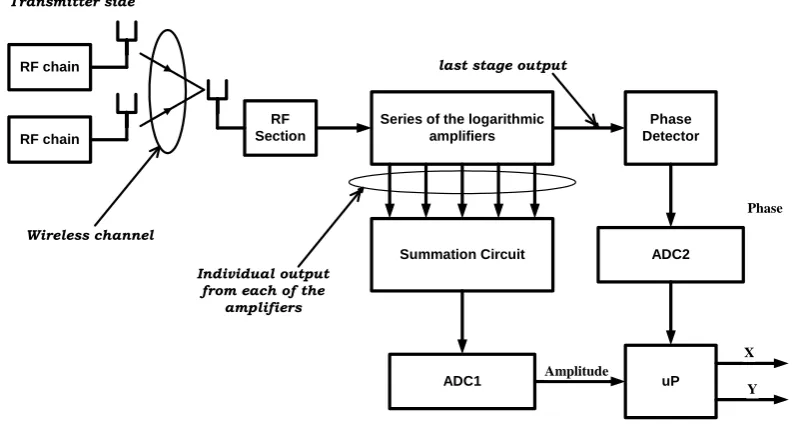
Paul Wilkinson of Ericsson® has proposed to use a Log-Polar receiver structure for the described scenario [19]. It uses logarithmic amplifiers to increase the acceptable range of the input signals at the expense of the introduced signal distortion. Figure 7 shows the schematic diagram of the receiver.

RF Section

Series of the logarithmic amplifiers

Summation Circuit

Phase Detector

ADC1 uP

RF chain

RF chain

Wireless channel Transmitter side

Individual output from each of the

amplifiers

Phase

Amplitude

last stage output

X

Y

ADC2

After the RF stage, the signal passes through a series of logarithmic amplifiers. Each amplifier is designed to saturate every 1dB (relative to the input voltage) increase in the voltage level. The last amplifier in the chain is saturated first, followed by the preceding amplifier and so on. Thus the maximum possible input signal level is limited by the number of the amplifier stages. The outputs of the individual amplifiers are summed to obtain the total log-magnitude value of the signal. The logarithmically processed signal enables ADC1 in figure 7 to accommodate large swings in the amplitude of the incoming signal. The downside, however, is that the signal becomes exponentially distorted (the signal is compressed harder as its amplitude grows). The digitised signal magnitude is then fed into a microprocessor. The output of the last amplifier is also applied to a phase detector, which then extracts the phase information out of the received signal (the phase value is retained even when the signal is hard clipped due to the amplifier saturation). The phase value is converted into a digital form by the second ADC (ADC2) and is also fed into a microprocessor. The task of the microprocessor is to convert the Polar representation of the signal into the Cartesian one. This receiver structure is most suitable for the phase-modulated schemes (like M-PSK), where the introduced distortion of the magnitude of the signal does not affect the system performance.

3.2.3 Signal conversion

Figure 8 shows the equivalent representation of ADC

Figure 8. ADC broken down into a sampler and quantiser

ADC consists of two major parts. First, the input analog waveform has to be sampled at a frequency at least twice as high as the bandwidth of the input waveform to avoid aliasing [21]. Then incoming samples are quantised into discrete levels and binary encoded. For an ADC with A bits and

full-scale range VF,q – the size of the quantisation step is given by

2 1 2

F F

A A

V V q= ≈

− (19)

Signal quantisation induces a quantisation error ε in the system. It has a uniform distribution in the

range 2

q

± . Then its power σ_ε2 can be calculated

( )

2 2 2

2

2 2 2 2

2

;

1

12

q

q

q

q

p d

q d q

ε

ε

σ ε ε ε

σ ε ε

−

−

= ∗

= =

∫

∫

(20)

The dynamic range of an ADC is defined as the ratio between the maximum to minimum levels the ADC can accept. With the maximum level as VF, the minimum level as q, the dynamic

range D is

( )

2 ; 2

[ ] 20 log 2

A

F F

F A

A

V V D

q V

D dB

= = =

⎛ ⎞

⎜ ⎟

⎝ ⎠

= ∗

(21)

The more bits the ADC has, the higher its dynamic range; that is, the wider the range of signal amplitudes it can handle.

Reducing the dynamic range will reduce the power consumption of the ADC at the expense of increased quantisation noise. The maximum voltage level VF can subsequently be lowered to

counteract the increased quantisation noise. However, there is then an increased risk of signal clipping by the ADC, because it is more likely that the maximum signal amplitude can exceed VF.

The signal, distorted by the clipping, impairs the overall performance of the system. It is possible to optimise the ADC power consumption by choosing the lowest number of bits and the lowest VF for

certain Symbol Error Rate (SER).

The rest of the chapter comprises novel work that investigates the performance deterioration of the Alamouti STBC structure employing two transmit and one receive antennas in the presence of ADC clipping in DC and Log Polar receivers for 10-3 target SER.

3.3

Clipping in SISO systems

3.3.1 DC receivers and square clipping

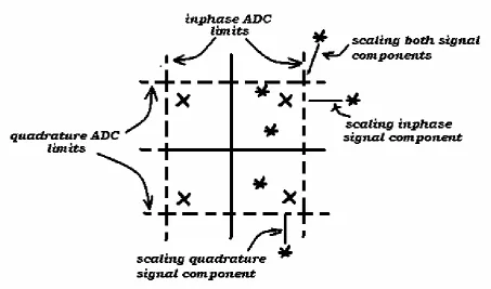
Figure 9. A conceptual example of the square clipping of a QPSK modulated signal

The square region in figure 9 is formed by the maximum acceptable signal amplitudes of the inphase and quadrature ADCs. Inside this bounded region four original signal constellations are shown ("X"es in the figure). The received signal (represented by stars in figure 9) outside of this region is scaled (or clipped) by ADCs. The soft limiting operation of each ADC is shown in the figure below

At any time instant t,clipping either the inphase or quadrature branch of the complex signal

can be represented as follows:

( )

( )

( )

( )

( )

( )

y t y t r

r t

y t y t r

r

y t

α

α

(22)

In (22) and in figure 10, y(t) is a received signal before the clipping and r(t) is a signal after the clipping. Following the definition in (22), the scaling coefficient α has the following properties:

1, ( )

, ( ) ( ) ⎧ < ⎪ = ⎨ ≥ ⎪ ⎩ clip clip clip

y t r r

y t r y t

α (23)

Two ADC converters operate independently on inphase and quadrature parts of the complex input signal. Then the received signal can be shown as:

(

)

(

)

(

)

(

)

[

]

(

)

i r i i r i r i i r r r n j n h s h s j h s h s r n h s h s j n h s h s r ∗ ∗ + ∗ + ∗ + ∗ ∗ ∗ + ∗ − ∗ = + ∗ + ∗ ∗ + + ∗ − ∗ = ∗ ∗ ∗

α

α

α

α

α

α

In (24) reference to time is omitted; s=sr+jsi is a transmitted symbol; h=hr+jhi is a sample of

the complex i.i.d channel; n=nr+jni represents a complex noise snapshot; αr and αi are clipping

coefficients of the inphase and quadrature branches respectively.

3.3.2 Log-Polar receivers and circular clipping

Figure 11. Magnitude clipping in a Log-Polar receiver employing QPSK modulation

The full-scale range of ADC1 in figure 7 forms a circular boundary on the Cartesian plane in figure 11. The ADC clips (or scales) all the complex signals whose magnitude exceeds this boundary. The soft clipping operation of this ADC is presented in figure 12

Figure 12. Soft limiting operation of the ADC in a Log-Polar receiver

(

)

r =

α

Here, reference to time is omitted; both the real and imaginary components of r are scaled

equally by α.

The next section will use the defined scaling coefficient to investigate clipping effects in the DC and Log-Polar receivers that employ STBC.

3.4

Clipping in Alamouti STBC System

3.4.1 Square clipping

The clipped form of the STBC signal is represented by

( )

(

)

(

)

( )

(

)

(

)

0 0 0 0 1 1 0 0 0 0 1 1 0

1 1 0 1 1 0 1 1 0 1 1 0 1

Re Im

Re Im

r i

r i

r t s h s h n j s h s h n

r t s h s h n j s h s h n

α α

α ∗ ∗ ∗ α ∗ ∗ ∗

= ∗ ∗ + ∗ + + ∗ ∗ ∗ + ∗ +

= ∗ ∗ − ∗ + + ∗ ∗ ∗ − ∗ + (26)

In (26) α0 is a scaling coefficient at time slot zero and α1 is a scaling coefficient at time slot

Defining:

(

)

(

)

(

)

2 2 2 2

0 0 0 1 1 0 0 0 1 1

2 2 2 2

1 1 0 0 1 0 1 0 0 1

0 1 0 1

! , ; ! ! , ; , ; = ∗ + ∗ = ∗ + ∗ − = ∗ + ∗ = ∗ + ∗ = − = −

r r r i i i

r r r i i i

r r r i i i

n

h h h h

r n r

h h h h

d d ρ α α ρ α α ρ α α ρ α α α α α α α α (27)

Then, after multiplying by transposed-conjugated channel matrix and further defining,

(

)

(

)

(

)

(

)

(

)

(

)

(

)

(

)

* *

0 0 1 1 1 0 1 1 1

* *

1 0 1 0 0 0 1 0 0

Re Im

Re Im

r r i i r i i r

r r i i r i i r

k h h d s j d s h h d s j d s

k h h d s j d s h h d s j d s

α α α α

α α α α

= ∗ ∗ ∗ + ∗ ∗ − ∗ ∗ ∗ + ∗ ∗

= ∗ ∗ ∗ + ∗ ∗ − ∗ ∗ ∗ + ∗ ∗

(28)

Symbol estimates then can be presented

(

)

(

)

(

)

(

)

* *

0 0 _{0 0 1}

* *

1 1 1 0 0 1

ˆ

0 0 0 0 1

ˆ

1 1 1 1

c c

c c

s s j s k h n h n r r i i

s s j s k h n h n r r i i

ρ ρ

ρ ρ

= ∗ + + + ∗ + ∗

= ∗ + + +

∗

∗ ∗ − ∗ (29)

Here n0c and n1c represent the Inphase Quadrature clipped noise in time slots zero and one

respectively.

STBC uses time as a coding domain. As a result of the coding, the two consecutive STBC samples become orthogonal. Clipping in the time domain will affect coding by breaking orthogonality between the samples. The terms k0 and k1 represent cross-talk terms, showing the

3.4.2 Circular clipping

The STBC signal, affected by the circular clipping, can be written as

(

)

(

)

0 0 0 0 1 1 0

1 1 0 1 1 0 1

t t

r s h s h n

r s h s h n

α

α ∗ ∗ ∗

= ∗ ∗ + ∗ +

= ∗ ∗ − ∗ + (30)

As in the case for square clipping, the top line defines the signal at the first time slot and the second line at the second time slot.

Defining

(

)

2 2

0 0 0 1 1

2 2

1 1 0 0 1

0 1 ; ; . r r r h h h h d ρ α α ρ α α α α α = ∗ + ∗ = ∗ + ∗ = − (31)

Since only the magnitude is clipped, k0 and k1 in (28) can be rewritten to suit the circular

clipping case

(

)

(

)

*

0 0 1 1

*

1 0 1 0

k d h h s

k d h h s

α

α

= ∗ ∗ ∗

= ∗ ∗ ∗

(32)

Finally, the symbol estimates are presented as

(

)

(

)

* * 0 0 0 0 _{0 0 1}

* *

1 1 1 1 1 0 0 1

ˆ

1 ˆ

c c

c c

s s k h n h n s s k h n h n

ρ

ρ

= + + ∗ + ∗

= + +

∗

∗ ∗ − ∗ (33)

Here the cross-talk terms k0 and k1 also appear, due to the orthogonality loss in the coding.

3.5

Simulations and Comparisons

Figure 13. Simulation block diagram

Figure 13 shows the block diagram and specifies all the necessary parameters used to produce the simulation results. The channel is ideally estimated at the receiver, and assumed to be flat fading, having complex Gaussian Independent Identically Distributed (i.i.d) samples. All the clip values are taken relative to the received signal Root Mean Square (rms) value (without the noise).

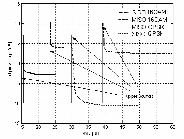
Figure 14 shows the lowest possible clipping levels at different SNR values, while maintaining target 10-3 SER for square clipping: STBC QPSK, STBC 16QAM, SISO QPSK and SISO 16QAM. For all four schemes, inter-symbol-interference (ISI) caused by Root Raised Cosine (RRC) filters is one of the error contributors besides AWGN. For STBC schemes, however, the cross-talk noise is another major contributor of the error. This is the reason for the STBC signal clip floor being 1dB higher than the clipping floor of the SISO scheme for 16QAM modulation. This difference expands to 7dB for the QPSK system, as depicted in figure 14. STBC systems perform 15 dB better when compared to SISO schemes for the same clipping levels. This is true for both constellation densities used for this research.

For the circular clipping scenario (STBC system with QPSK modulation), the unrealistically low clipping level of –30dB was found to induce a symbol error rate of 3*10-4, way below the target SER of 10-3_{. The Log-Polar receiver structure is essentially clipping insensitive at this particular}

target SER.

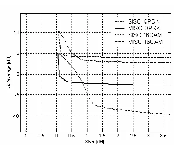
Figure 15. Sensitivity of STBC and SISO schemes to AWGN at 10-3 target SER, DC

receaver, square clipping.

This plot is built by lining up the upper bounds of all schemes to zero. The amount of SNR required for every scheme to achieve its clip floor can be defined as the noise sensitivity of the scheme.

It takes about 0.5 dB of change in SNR for the STBC system to achieve its clip floor (QPSK and 16QAM). This value is 1dB for SISO 16QAM and about 9dB for SISO QPSK. It is also important to note in figure 15 that from 0 to 0.5 dB for 16QAM and from 0 to 0.7 dB for QPSK, STBC schemes have lower clip levels, making them superior to SISO schemes within this SNR range.

3.6 Conclusions

receiver structures were considered: the DC receiver structure that employs two ADCs on the inphase and quadrature branches and the Log-Polar receiver that recovers the complex envelope in the polar form. It has one ADC to digitise the magnitude and another one to digitise the phase of the received signal. The two independently operating ADCs in a DC receiver induce a square clipping, while an ADC that digitises the signal magnitude in a Log-Polar receiver causes a circular clipping on the Cartesian plane.

STBC rely on orthogonal coding to separate individual symbols. It was shown that ADC clipping leads to breaking the code orthogonality. As a result, cross-talk interference can adversely affect the performance of the system. For the square clipping case, simulations have confirmed that STBC schemes have a higher clip floor and are more sensitive to AWGN than SISO systems. For receiver designers this means that they must increase signal back off into ADC by 7 dB for QPSK and 1 dB for 16QAM with Alamouti STBC scheme.

4 Complexity Reduction through Upper Triangular Matrix

Tracking in QR Detection MIMO Receivers

4.1 Chapter

Outline

triangular matrix tracking does not show any BER advantage over the channel-tracking scenario and also results in a higher computational complexity. Both LMS channel tracking schemes are then compared with the RLS-DFE tracking system of [1]. The equalizer coefficients (inverse channel) exhibit higher dynamics than the channel and suggest the possibility of using lower complexity tracking schemes. Both LMS strategies had an inferior BER performance compared to the DFE RLS-based system, and surprisingly the LMS schemes showed no significant complexity improvement. The work has been published in [72]. The chapter is organised as follows.

Section 4.2 introduces the 802.11n channel model, reviews existing detection and estimation techniques in MIMO, explains the importance of tracking in MIMO systems and formulates the problem.

Section 4.3 describes two tracking strategies and compares their performance based on the MSE of the channel-estimate metric. The section also reviews the application of the CORDIC algorithm to QRD and highlights potential modifications that can be exploited when the target matrix is nearly upper triangular.

The BER performance of both channel and upper triangular matrix tracking strategies with SIC-MMSE detection is presented in section 4.4.

Finally, section 4.5 draws the conclusion to the chapter.

4.2 Introduction

4.2.1 IEEE 802.11 TGn channel model

spectrum, angle spread, mean angle of departure and arrival determine the degree of correlation [22].

Channel models are developed for the standard indoor A-F environments (for instance, A is flat fading, B is residential, etc.). This model uses the following formula to describe the Doppler spectrum of the signal

2

1 ( )

1 9 c d

S f

f f f

=

⎛ − ⎞

+ ∗⎜ ⎟

⎝ ⎠

(34)

The Doppler frequency fd was experimentally determined to be 6Hz for the indoor

environment [22]. This model assumes near-stationary transmitters and receivers and moving scatterers. An example could be an office environment, where the access point and notebooks are stationary and walking people are scatterers. The F environment was selected for this work because it had the highest Doppler spread. It includes one fast-moving scatterer at 40km/h. Practically, this can be a car moving outside the office window.

Figure 16a compares the Doppler spectrum of the 802.11n models A to E to Clarke's model [4]. The frequency spectrum from the right of the carrier frequency fc is plotted for both cases.

0 5 10 15 20 25 30 0 0.1 0.2 0.3 0.4 0.5 0.6 0.7 0.8 0.9 1

Doppler spectrums: 802.11n model and Clarke's models

(f-f

c) frequency [Hz]

P o w e r D e n s it y S p ect ru m S (f -f c ) Clarke's model 802.11n indoor f d=6Hz (a)

0 50 100 150 200 250

-100 -80 -60 -40 -20 0 20

(f-fc) frequency [Hz]

Po w e r D e n s it y Sp e c tr u m S (f-f c ) [d B ]

PSD of the Doppler 802.11n F model

(b)

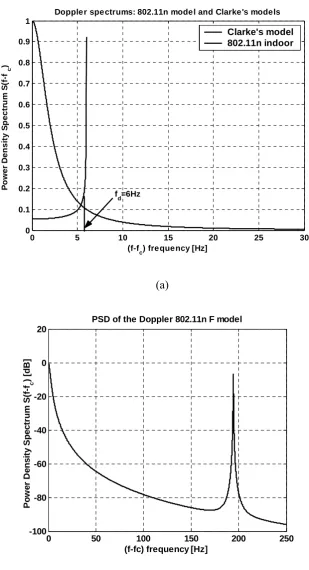
Figure 16. (a) Doppler spectra used in 802.11n and Clarke's models (b) 40km/h moving object

It can be observed from figure 16a that unlike Clarke's model, where most of the power spectrum is contained in the frequency components close to fd, most of the power spectrum in

802.11n is retained around the carrier frequency fc. Also the 802.11n curve is truncated at fmax of five

times the Doppler frequency (30KHz in our case). In the case of channel F (figure 16b) the moving cluster causes a significant amount of energy at 194Hz.

4.2.2 Detection in MIMO

MIMO systems offer high theoretical information capacities. Spatial multiplexing is used to achieve these high capacities, as stated in chapter 2. There are various ways to perform symbol detection in spatial multiplexing systems, and this sub-section will describe some of them.

The received baseband NX1 signal vector yi at ith time instant can be expressed as

= +

i i i

y Hs n (35)

where H is an NXM channel matrix assumed known at the receiver, si is M X 1 transmitted signal

vector, ni is an NX1 additive WGN vector where each element is distributed as N

( )

For the constellation of sizeθ ,the set of all possible constellation symbols is defined

asK_θ =

{

}

The optimum Maximum Likelihood Sequence Detector (MLSD) [6] finds Euclidean distances between the received signal vector yi and all the possible sequences of transmitted symbol

vectors distorted by the channel. Then the symbol vector, corresponding to the minimum distance is

chosen as an estimate of the transmitted symbol vector ˆs_i.

(

)

ˆ arg min

∈

=

i i

s y - HT

M

T Kθ

where K_θM is a space of all the available sequences.

There are θM _{possible sequences that MLSD has to consider to make a choice. The}

complexity increases exponentially with the number of antennas, which severely restricts its use in practical systems. Less complex, suboptimum detectors are described in the following sub-sections.

4.2.2.1 Linear detectors

Linear detectors obtain the estimate of the transmitted symbol via linear mapping

(

)

ˆ_i = _i

s ϑ Ay where ϑ

( )

criteria:

1. ZF criteria [24]:_{A = H}-1_{. Symbol estimate is then}

ˆ -1 -1

i i

s = Ay = H Hs + H n (37)

Defining error covariance matrix as

(

)(

)

⎡ ⎤

= ⎣ i i i i H⎦

P E s - s s - s (38)

For the ZF case

(

)(

)

(

)

⎡ ⎤

= _⎣ -1 H -H _⎦= H

i i i i i i

P E s - s - H n s - s - n H σ_n H H (39)

The WGN noise amount in the symbol vector estimate will be amplified by small

eigenvalues,

(

)

H H that occur when the channel is faded or ill conditioned. It was shown in

[25-27] that ZF detection with Bit Interleaved Coded Modulation (BICM) can asymptotically achieve ML performance as the number of antennas grows to infinity.

2

ˆ

⎡ ⎤

=E_⎣s_i−s_{i ⎦}

ε (40)

After presenting the symbol vector estimate ˆs_i as a linear combination of the received signal

vector yi, error ε can be minimised in the linear sense

1

2 min arg min

∈ℜ ⎡ ⎤ = _⎢ − _⎥ ⎣ ⎦ H i i

s A y

NX

A

E

ε (41)

The optimum (in linear MMSE sense) Aopt that corresponds to minimum error can be derived

as

(

)

opt i i i i

opt NXN

A y y y s

A I HH H

H H H n s E E σ σ (42)

where 2

s

σ is a signal power.

The error covariance matrix is obtained as follows [28]

( )( )

(

)

2 2

ˆ ˆ ;

−

⎡ ⎤

= ⎣ ⎦

= _MXM+

s - s s - s

I H H

H

H n n

P E P σ σ

(43)

where the signal is assumed to have a unit power.

Since the noise power is included in the inversion term, small eigenvalues of H HH will not

result in large noise amplification in the symbol vector estimate. MMSE detection in MIMO is used in [29, 30].

Importantly, for both ZF and MMSE methods the amount of noise amplification in the

symbol vector estimate will be dominated by the smallest eigenvalue in

(

)

(

)

MXM

I H HH

n