Segmentation Techniques: A Comparison and Evaluation on MR Images for Brain Tumour Detection

Volume 7, No. 2, March-April 2016

International Journal of Advanced Research in Computer Science

REVIEW ARTICLE

Available Online at www.ijarcs.info

Segmentation Techniques: A Comparison and Evaluation on MR Images for Brain

Tumour Detection

A.R. Jasmine Begum

Dr.T. Abdul Razak

Assistant Professor, Dept. of Information Tech. Associate Professor, Dept. of Computer Science Cauvery College for women Jamal Mohamed College

Tiruchirapalli-620 018 Tiruchirapalli-620 020

Abstract: Brain tumour is inherently serious and life-threatening because of its character in the constrained space of the intracranial cavity (space formed inside the skull). If the tumour is detected at an advanced stage it turns to be a grave medical problem. Various techniques were developed for the detection of brain tumour. The image segmentation technique plays a pivotal role in early tumour detection. The segmentation is the process that partitions an image into regions. The widely used common image segmentation techniques are edge detection and clustering techniques.

Edges cause significant local changes in the image intensity and have been an important feature for analysing images. It is the first step in receiving information from images. The techniques discussed here are Gradient-based methods such as Roberts, Sobel, Prewitt, Canny operators and Laplacian based edge detection method such as Laplacian of Gaussian operator(LOG). Clustering is the method of grouping a set of patterns into a number of clusters. The two important clustering algorithms namely centroid based K-Means and representative object based Fuzzy C-Means (FCM) clustering algorithms are compared.

This paper presents the qualitative comparison of edge detection and clustering techniques for brain tumour MRI images based on image quality parameters like PSNR (Peak Signal to Noise Ratio), MSE (Mean Square Error), RMSE (Root Mean Square Error) and computing time.

Keywords: Gradient-based, Laplacian, K-Means, Fuzzy C-Means, PSNR, MSE, RMSE, Computing time.

I INTRODUCTION

Image enhancement is the task of applying defined transformations to an image to acquire a visually more pleasant cum detailed or less noisy images as an output. Brain tumour detection and its analysis is a challenging task in medical image processing because brain image is complicated.

The brain is the most important part of central nervous system. Brain tumour is an intracranial solid neoplasm. The main task of the doctor is to detect the tumour which is a time consuming, which makes them feel burden. The optimal solution for this problem is the prudent usage of Image Segmentation.

The purpose of Image Segmentation is to partition on image into meaningful regions with respect to a particular application. Image Segmentation is classified as follows into two categories on the grounds of image property as shown in the Figure 1.1

• Based on Discontinuity • Based on Similarity[1]

Edge detection is the operation of detecting local changes in an image. Edge in an image is associated with a discontinuity in the image intensity. It can be either

• Step discontinuity- Image intensity abruptly changes from one value to a different value.

• Linear discontinuity- Image intensity abruptly changes but then returns to the starting value within some short distance.

The principal approaches in the similarity category are based on partitioning an image into regions that are similar

according to a set of predefined criteria. Thersholding, Region growing, Region splitting and Merging are examples for this category [1].

Image segmentation can be performed effectively by clustering image pixels. Cluster analysis allows the partitioning of data into meaningful subgroups and it can be applied for image segmentation or classification purposes. K-Means is a simplest unsupervised learning technique that solves the most recurring clustering problem. It is an algorithm to classify or to group your objects based on features into K number of group.

Fuzzy C-Means (FCM) is a method of unsupervised clustering algorithm which allows one piece of data to belong to two or more clusters. Figure 1.1 illustrates various image segmentation techniques, this paper focuses on edge detection techniques and feature based clustering techniques among them.

A. Edge Detection Techniques

Edge detection refers to the process of identifying and locating sharp discontinuities in an image. There are different methods are used for edge detection and it is grouped into two categories [3].

• Gradient: The gradient method detects the edges by looking for the maximum and minimum in the first derivative of the image.

• Laplacian: The Laplacian method searches for zero crossings in the second derivative of the image to find edges.

B. Steps in Edge Detection

Filtering-Filtering are commonly used to improve the performance of an edge detector with respect to noise.

• Enhancement- Enhancement emphasizes pixels where there is a significant change in local intensity values and is usually performed by computing the gradient magnitude.

• Detection- This Method is applied to determine which points are edge points. Frequently, thresholding provides the criterion used for detection. • Localization- The location of the edge can be

estimated with sub-pixel resolution if required for the application [3].

In this paper various Edge detecting operators such as Sobel’s, Robert’s, Prewitt’s, Canny and Clustering algorithms such as K-Means, Fuzzy C-Means are compared using various quantitative measures.

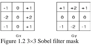
C. Sobel’s Operator

The Sobel operator performs a 2-D spatial gradient measurement on an image and so emphasizes regions of high spatial gradient that correspond to edges. Typically it is used to find the approximate absolute gradient magnitude at each point in an input gray scale image [4].

The operator consists of a pair of 3×3 convolution kernels as shown in Figure 1.2 One kernel is simply the other rotated by 90°.

Figure 1.2 3×3 Sobel filter mask

These masks are designed to respond maximally to edges running vertically and horizontally relative to the pixel grid and it can be applied separately to the input image, to produce separate measurements of the gradient component in each orientation (call these Gx and Gy). These can then be combined together to find the absolute magnitude of the gradient at each point and the orientation of that gradient. The gradient magnitude is given in the eqn.1.

|𝐺𝐺| =�𝐺𝐺𝑥𝑥2+𝐺𝐺𝑦𝑦2 (1)

The angle of orientation of the edge (relative to the pixel grid) giving rise to the spatial gradient is given in the eqn.2

𝜃𝜃= arctan⁡(𝑮𝑮_𝑮𝑮𝒚𝒚

𝒙𝒙) (2)

D. Robert’s Operator

The Roberts Cross operator performs a simple, quick to compute, 2-D spatial gradient measurement on an image. Pixel values at each point in the output represent the estimated absolute magnitude of the spatial gradient of the input image at that point [5].

Figure 1.3 2×2 Roberts filter mask

The operator consists of a pair of 2×2 convolution kernels as shown in Figure 1.3.This is very similar to the Sobel operator.

The kernels can be applied separately to the input image, to produce separate measurements of the gradient component in each orientation. (call these Gx and Gy). These can then be combined together to find the absolute magnitude of the gradient at each point and the orientation of that

gradient. The gradient magnitude is given in the Equation 3.

|𝐺𝐺| =�𝐺𝐺𝑥𝑥2+𝐺𝐺𝑦𝑦2 (3)

𝐺𝐺𝑥𝑥 ,𝐺𝐺𝑦𝑦 gradient components

The angle of orientation of the edge (relative to the pixel grid) giving rise to the spatial gradient is given in Equation 4.

𝜃𝜃= arctan⁡(𝑮𝑮𝒚𝒚_𝑮𝑮

𝒙𝒙)-3п/4 (4)

E. Prewitt’s operator

Prewitt operator is similar to the Sobel operator and is used for detecting vertical and horizontal edges in images. The operator consists of a pair of 3×3 convolution kernels as shown in Figure 1.4

ℎ1=�

1 1 1

0 0 0

−1 −1 −1� ℎ2=�

−1 0 1

−1 0 1

−1 0 1�

Figure 1.4 3×3 Prewitt filter mask

The maximum response of all 8 kernels for a pixel location is used to calculate the local edge gradient magnitude

|G| = max (|Gi|: i=1 to n)

Gi-The response of the kernel i at the appropriate pixel position, n -The number of convolution kernels. Unlike the Sobel operator, this operator does not place any emphasis on pixels that are closer to the center of the masks [5].

F. Canny Operator

The Canny operator has been designed to be an optimal edge detector. It takes as input a grey scale image, and produces as output an image showing the positions of tracked intensity discontinuities. The Canny operator works in a multi-stage process. First of all the image is smoothed by Gaussian convolution as given in the Equation 5. [3].

Where S [i, j] smoothed array, G [i, j] Gaussian filter, I [i, j] image.

𝑃𝑃[𝑖𝑖,𝑗𝑗]≈(𝑆𝑆[𝑖𝑖,𝑗𝑗] +𝑆𝑆[𝑖𝑖+ 1,𝑗𝑗+ 1]− 𝑆𝑆[𝑖𝑖+ 1,𝑗𝑗])/2 (6)

Where P [i, j] partial derivatives of x.

𝑄𝑄[𝑖𝑖,𝑗𝑗]≈ 𝑆𝑆[𝑖𝑖,𝑗𝑗]− 𝑆𝑆[𝑖𝑖+ 1,𝑗𝑗] +𝑆𝑆[𝑖𝑖,𝑗𝑗+ 1]− 𝑆𝑆[𝑖𝑖+ 1,𝑗𝑗+ 1])/2 (7) Where Q [i, j] partial derivatives of y.

𝑀𝑀[𝑖𝑖,𝑗𝑗] =�𝑃𝑃[𝑖𝑖,𝑗𝑗]2_{+𝑄𝑄[𝑖𝑖,𝑗𝑗]}2 ₍₈₎

Where M [i, j] magnitude array

𝜃𝜃= arctan⁡(𝑄𝑄[𝑖𝑖,𝑗𝑗],𝑃𝑃[𝑖𝑖,𝑗𝑗] (9)

This algorithm then tracks along the top of these ridges and sets to zero all pixels that are not actually on the ridge top so as to give a thin line in the output, the process known as non-maximal suppression and is defined in the following Equations 10 and 11.

ℶ[𝑖𝑖,𝑗𝑗] =𝑠𝑠𝑠𝑠𝑠𝑠𝑠𝑠𝑠𝑠𝑠𝑠(𝜃𝜃[𝑖𝑖,𝑗𝑗]) (10) 𝑁𝑁[𝑖𝑖,𝑗𝑗] =𝑛𝑛𝑛𝑛𝑠𝑠(𝑀𝑀[𝑖𝑖,𝑗𝑗],ℶ[𝑖𝑖,𝑗𝑗] (11)

Where ℶ[𝑖𝑖,𝑗𝑗] sector value

𝜃𝜃[𝑖𝑖,𝑗𝑗] angle of the gradient

The tracking process exhibits hysteresis controlled by two thresholds: T1 and T2 with T1 > T2. Tracking can only begin at a point on a ridge higher than T1. Tracking then continues in both directions out from that point until the height of the ridge falls below T2. This hysteresis helps to ensure that noisy edges are not broken up into multiple edge fragments [6].

G. Laplacian of Gaussian(LoG)

The Laplacian is a 2-D isotropic measure of the 2nd spatial derivative of an image. The Laplacian of an image highlights regions of rapid intensity change and is therefore often used for edge detection. It is often applied to an image that has first been smoothed with a G in order to reduce its sensitivity to noise. The Laplacian L(x,y) of an image with pixel intensity values I(x,y) is given by in the Equation 12 [6].

𝐿𝐿(𝑥𝑥,𝑦𝑦) = 𝜕𝜕2_𝐼𝐼 𝜕𝜕𝑥𝑥2+

𝜕𝜕2_𝐼𝐼

𝜕𝜕𝑦𝑦2 (12) Three commonly used small kernels are shown in Figure 1.5

Figure 1.5 Three commonly used discrete approximations to the Laplacian filter.[6]

II CLUSTERING TECHNIQUES

The clustering algorithms groups a sample set of feature vectors into K clusters via an appropriate similarity or dissimilarity criterion.

A. K-Means Algorithm(KM)

K-Means algorithm iteratively computes cluster centroids for each distance measure in order to minimize the sum with respect to the specified measure. KM algorithm aims at minimizing an objective function known as squared error function [7].

The algorithm for the K-Means clustering is as follows:

1. Initialize number of cluster and centre

2. For each pixel of an image, calculate the Eucledian distance d between the center and each pixel of an image using the equation given below

= ‖p(x,y)−ck‖ (13) 3. Assign all the pixels to the nearest center based on distance d.

4. After all pixels have been assigned, recalculate new position of center using the equation given below

𝑣𝑣𝑖𝑖= 1� ∑𝑘𝑘 𝑦𝑦∈𝑠𝑠𝑘𝑘∑𝑥𝑥∈𝑠𝑠𝑘𝑘𝑝𝑝(𝑥𝑥,𝑦𝑦) (14)

5. Repeat the process until it satisfies the error value. 6. Reshape the cluster pixels into image [7].

B. Fuzzy C-Means Algorithm(FCM)

Fuzzy C-Means Clustering is separate from K-Means that employs hard partitioning. FCM algorithm minimizes the objective function in Equation (15) [9].

𝐽𝐽𝐹𝐹𝐹𝐹𝑀𝑀(𝑋𝑋;𝑈𝑈,𝑉𝑉) =∑𝑗𝑗𝑛𝑛=1∑𝑠𝑠𝑖𝑖=1𝑢𝑢𝑖𝑖𝑗𝑗𝑛𝑛𝐷𝐷2𝑖𝑖𝑗𝑗𝑖𝑖 (15)

This function differs from classical KM with the use of weighted squared errors instead of using squared errors only. In the objective function in Equation (15), 𝑼𝑼 is a fuzzy partition matrix that is computed from dataset 𝑿𝑿:

𝐔𝐔=[uij]∈𝑀𝑀FCM

FCM is an iterative process and stops when the number of iterations is reached to maximum, or when the difference between two consecutive values of objective function is less than a predefined convergence value (𝜀𝜀).The steps involved in FCM are [8]:

1) Initialize (0) membership matrix randomly. 2) Calculate prototype vectors:

𝑣𝑣𝑖𝑖 =

∑𝑛𝑛𝑗𝑗=1𝑢𝑢𝑖𝑖𝑗𝑗𝑛𝑛𝑥𝑥𝑗𝑗

∑𝑛𝑛𝑗𝑗=1𝑢𝑢𝑖𝑖𝑗𝑗𝑛𝑛 ;

1

≤𝑖𝑖≤𝑠𝑠

3) Calculate membership values with: 𝑢𝑢𝑖𝑖𝑗𝑗 =_{∑ (𝐷𝐷𝑖𝑖𝑗𝑗𝑖𝑖⁄𝐷𝐷}1

𝑘𝑘𝑗𝑗𝑖𝑖)2 (𝑛𝑛 −1)⁄ 𝑛𝑛

𝑗𝑗=1 1≤𝑖𝑖≤𝑠𝑠 ,1≤𝑗𝑗≤𝑛𝑛(17)

4) Compare 𝑼𝑼(𝑠𝑠+1) with 𝑼𝑼(𝑠𝑠), where 𝑠𝑠 is the iteration number

5) If ‖𝑼𝑼(𝑠𝑠+1)−𝑼𝑼(𝑠𝑠)‖<𝜀𝜀 then stop else return to the step 2. Where 𝐷𝐷2𝑖𝑖𝑗𝑗𝑖𝑖 is the distances between ith features vector and the centroid of jth cluster. They are computed as a squared inner-product distance norm in Equation 18.

𝐷𝐷2

𝑖𝑖𝑗𝑗𝑖𝑖=‖xj−vi‖𝑖𝑖2=(𝐱𝐱𝑗𝑗−𝐯𝐯𝑖𝑖)𝑇𝑇𝑨𝑨(𝐱𝐱_𝑗𝑗−𝐯𝐯_𝑖𝑖) (18)

The objective function is minimized with the constraints as follows [8]:

∈[0,1]; 1≤𝑖𝑖≤𝑠𝑠,1≤𝑗𝑗≤𝑛𝑛

� 𝑢𝑢𝑖𝑖𝑗𝑗 𝑠𝑠

𝑖𝑖=1 i=1; 1≤𝑗𝑗≤𝑛𝑛

0< � 𝑢𝑢𝑖𝑖𝑗𝑗

𝑠𝑠

𝑖𝑖=1 <n; 1≤𝑖𝑖≤𝑠𝑠

III QUALITY METRICS

Image quality is a characteristic of an image that measures the perceived image degradation. It plays a central role in various image processing applications.

A. Peak Signal to Noise Ratio (PSNR)

an image and a power of corrupting noise. The PSNR is

provided in decibel units (dB), it is defined as in Equation 19.

𝑃𝑃𝑆𝑆𝑁𝑁𝑃𝑃= 10𝑙𝑙𝑠𝑠𝑙𝑙10�(𝐿𝐿−1)

2

𝑀𝑀𝑆𝑆𝑀𝑀 � (19)

where L is the largest possible value of the signal (typically 255), Higher PSNR means more noise removed [9].

B. Root Mean Square Error (RMSE)

The Root Mean Square Error (RMSE) is being used as a standard statistical metric to measure average model-prediction error in the units of the variable of interest [9].

RMSE is an absolute measure of fit and it is the measure of average error based on the sum of squared errors. The RMSE is ideal if it is small [9]. It is defined in the following Equation 20.

𝑃𝑃𝑀𝑀𝑆𝑆𝑀𝑀=√𝑀𝑀𝑆𝑆𝑀𝑀=�_{𝑁𝑁𝑀𝑀}1 ∑ ∑𝑀𝑀−1(𝑖𝑖(𝑖𝑖,𝑗𝑗)− 𝐵𝐵(𝑖𝑖,𝑗𝑗))2

𝑗𝑗=0

𝑁𝑁−1

𝑖𝑖=0 (20)

where Mand N are the width and height of the image respectively, A is the original image and B is the distorted image.

IV EXPERIMENTAL RESULTS AND

DISCUSSION

The performance of the five edge detectors Sobel, Prewitt, Roberts, Canny, Laplacian of Gaussian(LoG) and Clustering techniques K-means and Fuzzy C-Means algorithms are compared based on the measures PSNR,MSE, RMSE and computing time on MR Image of brain tumour using MATLAB is shown in the Figures ranging from 1.6 to 1.10.

When comparing the performance between Clustering techniques, K-means and Fuzzy C-Means algorithms and Edge detection techniques, Sobel, Prewitt, Robert, Canny, Laplacian of Gaussian, Fuzzy C-Means algorithm is able to generate best results by showing high PSNR, low RMSE and MSE values. Because of the fuzzy measures calculations involved in the algorithm there is a slight increase in computation time than other techniques.

(a) (b) (c)

(d) (e) (f)

(g) (h) (i)

Figure1.6 Comparison between various Edge detection and Clustering Techniques (a) Original image; (b) Sobel (c) Prewitt (d) Robert (e) Canny (f) LoG (h) K-Means(i) Fuzzy C-Means.

Table-I Comparing the Performance Of Edge Detectors and Clustering Techniques on Brain Tumor MR Image

Figure1.8 Comparing RMSE of Edge detection and Clutering Techniques.

Figure1.9 Comparing MSE of Edge detection and Clutering Techniques

Figure1.10 Comparing Elapsed Time of edge detection and Clutering Techniques

V CONCLUSION

Edges are one of the most important elements in image analysis and computer vision, because they play quite a

significant role in many applications of image processing. This paper discusses a comparative study of five edge detection operators such as Sobel,Roberts,Prewitt,Canny, LoG and two clustering techniques K-Means and Fuzzy C-Means algorithm are processed. Their performance is valuated by applying on MR Image of brain tumour with four measures like PSNR,RMSE,MSE and elapsed time. Among all these techniques Fuzzy C-Means is showing the best results for PSNR,RMSE and MSE in detecting the brain tumour. But the execution time is higher for Fuzzy C-Means algorithm compared to other techniques because of the fuzzy measures calculations involved in the algorithm.. As future work the elapsed time of Fuzzy C-Means can be modified to reduce the elapsed time.

VI REFERENCES

[1] Gonzalez , R.C., Woods, R.E, Book on “Digital Image Processing”, 2nd Ed, Prentice-Hall of India Pvt. Ltd.

[2] P. Sujatha, K. K. Sudha2,Performance Analysis of Different Edge Detection Techniques for Image Segmentation, Indian Journal of Science and Technology, ISSN (Print) : 0974-6846, ISSN (Online) : 0974-5645,Vol: 8(14), IPL026, pp:, July 2015.

[3] Machine Vision, Edge Detection, chapter 5.

[4] Asra Aslama, Ekram Khanb, M.M. Sufyan Bega, Improved Edge Detection Algorithm for Brain Tumor Segmentation, Second International Symposium on Computer Vision and the Internet (VisionNet’15), Procedia Computer Science 58

( 2015 ), ISSN:1877-0509 ,pp:430 – 437, © 2015 Published by Elsevier B.V,2015.

[5] Akash Kumar Bhoi, Pradeep Kumar Mallick, S. Saravana Kumar, Karma Sonam Sherpa, Brain Tumor Detection: A

Comparative Analysis of Edge Detection Techniques, International Journal Of Applied Engineering Research, ISSN 0973-4562 Vol:10 Iss:44 pp:31569-31574,August 2015.

[6]

[7] Nameirakpam Dhanachandra, Khumanthem Manglem

and Yambem Jina Chanu, Image Segmentation using K-means Clustering Algorithm and Subtractive Clustering Algorithm, Eleventh International Multi-Conference on Information Processing-2015 (IMCIP-2015), Procedia Computer Science 54 ( 2015 ) ISSN:1877-0509© 2015 pp:764 – 771,2015. [8] Zeynel Cebeci, Figen Yildiz, ”Comparison of K-Means and Fuzzy C-Means Algorithms on Different Cluster Structures“, Journal of Agricultural Informatics (ISSN 2061-862X) 2015 Vol. 6,pp: 3:13-23,2015.

[9] G. Vishnuvarthanana, M. Pallikonda Rajasekaranb, P.Subbarajc, Anitha Vishnuvarthanand, An Unsupervised Learning Method with a Clustering Approach for Tumor identification and Tissue Segmentation in Magnetic Resonance Brain Images India Applied Soft Computing 38 (2016),ISSN: 1568-4946,© 2015 Elsevier B.V. pp:190– 212,2015.