DOI: http://dx.doi.org/10.26483/ijarcs.v9i1.5072
Volume 9, No. 1, January-February 2018
International Journal of Advanced Research in Computer Science
RESEARCH PAPER
Available Online at www.ijarcs.info
ISSN No. 0976-5697
CLASSIFICATION OF NETWORK VIOLATION DETECTION USING MACHINE
LEARNING
P.Syamala Rao
Research Scholar Dept. of Computer Science Acharya Nagarjuna University
Guntur, India
Dr. G.P.Saradhi Varma
Principal
Dept. of Information Technology, S.R.K.R Engineering College
Bhimavaram, India
Rajasekhar Mutukuri
Innovator
Dept. of Technology Center, S.R.K.R Engineering College
Bhimavaram, India
Abstract: Now a day’s Network Intrusion biggest issues in the internet services to solve this kind of issue we proposed a solutions to develop suitable IDS using (ML) Machine Learning algorithms. The pre-alter engine in IDS extracts significant characteristics from each network pattern connections. The central engine use which advanced characteristics as training input and outputs the binary analysis result, i.e., attack vs normal
Keywords: Network, Machine Learning, Networks pattern connections
1. INTRODUCTION
In present days, Network security is of extreme significance to Organization and every person. Most Advance technology is applying for defending the outgoing and incoming traffic, e.g. firewalls to prevent critical identities, encryption of sensitive data. Although they are the usual firewall and (IDS) Intrusion Detection Systems to identify and prevent them in uncertainty network transit based on pre-trained commands as well as models of known unusual attacks gathered in its database. This rise in size which is exponential from every network is complex.The legacy system is not of any use. On the other hand covered attack patterns pop-ups every time that makes it near to strange to keep the firewall upgrade.
In response to the objections, a higher firewall and/or IDS should prepare the following features. Firstly it should identify the systems unusual attacks very efficiently next it should be accessed unusual traffic patterns both industry and academia have been developing IDS performed with Machine Learning algorithms An exactly IDS represents the global pattern of normal against ill-disposed traffic, so able to present incoming traffic very faster than those returning to fixed status.
This project aims to develop suitable IDS using (ML) Machine Learning algorithms. The IDS pre-alter engine elicits vital features(payload size[PS],application service[AS],transport protocol[TP],connection duration[CD] from each network pattern connections. The central engine use which advanced.
Features as determining input and outputs the binary analysis result, i.e., attack vs. normal.
The rest of the article is classified as follows: Part 2 abstracts some relevant works. Part 3 addresses the data set and input characteristics in further details. Part 4 sets the execution Baseline using various single-stage classifier.
Part 5 aims an increase with more complicated multi-stage classification Algorithms. Part 6 directs on optimization with characteristic reduction. Part 7 ends the project with a matching of multiple implementations and moves directions for later development.
2. RELATED WORK
Given the fact that data in production to achieve in KDDCup’99[1] the data set has been implemented in the relevant field of super network security. As a data set must and should be clean data[2] set for the developing of good machine learning algorithm and also study of focusing techniques of normalization and raw data processing and also one way sabhnani processes one of the highly recommended feature reduction scheme which that results to improve classification results.
In Leonid Portnoy ET. al. [3] analyzing the datasets with K’ means clustering aims core relation between different attacks and the TLP (Transport Layer Protocol).
SVM with GA methods so that the most appropriate feature sets and excellent parameters of SVM could be known quickly. Chandrasekhar ET. al. [5] recommends a cascaded method using K-means clustering, Fuzzy-neural networks (FNN), and SVM.
3. DATA SET AND CHARACTERISTICS
Training and testing data sectors applied in this project were downloaded from the website raja434 GitHub page [6] the seasonal Data Mining and Information Discovery contest directed by ACM Special Interest Group. The network link records contains 41 feature fields and class field are generated by processing raw TCP dump data in a simulated Local Area Networks(LAN). The whole training set is produced from 7 weeks of network traffic, following in five million reports. The training and test data of a 10% subset was applied in this project.The system involves a training set of 495,048 samples and a test set of 312,057.
The data sample of each comprising of 41 features is classified into basic ,content and time-based features .The network connection points of a downloaded input set are of irregular format Some characteristics are thus converted from text to numerical value)or normalized to the corresponding order .The approaches of conversation are as below
• Text to numerical: feature fields specified with a text message such as service, protocol, etc.) are converted to integer values between 0 to 10
• .Medium numerical values: feature fields where the range of medium magnitude ˜102 are normalized to the range [0,10] w.r.t. its Maxville
• Large numerical values: feature fields where the numerical range is large ˜105 are converted to the range [0, 10] using base-10 logarithm.
Every training sample is known with a text intimating both normal and attack, with an accurate classification of the type of attack. The specific attack types can be additionally classified into four general categories. Thus ,the label united to give identity mapped integer values with
-[ normal(0),probing(1),DoS(2),R2L(4),U2R(3)].
4. SINGLE-STAGE CLASSIFIER
This section is with three single stage classifiers of Naive Bayes ,K-means clustering and Decision Tree which are trained and tested.The model parameters are selected by using Holdout cross validation at appropriate instant.The multi-class analysis is performed for each pattern,the result is obtained on the basis of difficulty matrix of attack (negative) VS normal (positive) described in Table I. In other words, misclassifications across various types of attacks are neglected as it does not raise any concern in the real utilization.
TABLE I: Confusion Matrix
True Positive Rate (TPR)
True normal predicted as normal
True Normal
False Positive Rate (FPR)
True attack predicted as normal
True Attack
False Negative Rate (FNR)
True normal predicted as attack
True Normal
True Negative Rate (TNR)
True attack predicted as attack
True Attack
A. Naive Bayes
Analysis with Naive Bayer’s algorithm is simple and effective, yet provides adequate results for most analysis problems. Therefore, it is performed as the baseline for other more superior algorithms. A trained Naive Bayes classifier uses Maximum A Later estimation to predict the class of test data P(Y) with known characteristics x1; x2;……. xn by
maximizing the conditional probability of P(y|x1,x2…….xn).
Bayes Theorem defines that:
Following the assumption that all characteristics are confident, Eq. 1 can be further decreased to:
Hence the MAP can be expressed as the
In extension, it is estimated that every characteristic reflects a Gaussian distribution as in Eq. 5 wherever the parameters µy
and σy are determined using best likelihood.
The barrier matrix of analysis result using the above multi-class Gaussian Naive Bayes multi-classifier is displayed in TableII
TABLE II: Confusion Matrix for Naive Bayes
TruePositiveRate = 0.9410 FlasePositiveRate = 0.9018 FlaseNegativeRate = 0.0592 TrueNegitiveRate = 0.9082
B. Decision Tree:
test unit starts from the source node and crosses through a selected path to a leaf node based on the judgment made at each node. In the training process each leaf node is identified and the same label as the leaf node is selected for the test sample.
Throughout the training process , the analysis criterion at each node is determined by maximizing information gain..
IG (Y|X) for a given node with trait X is defined as Entropy difference before and after distribution [7].
H(Y) is Entropy ere distribution, which includes the correlation of a distributed set of data as follows:
H(Y|X) is the weighted total of Entropy for all subsets later distribution based on Attribute X, determined as below:
Thus each node partitions the data set using the most different attribute by maximizing the Information Gain.
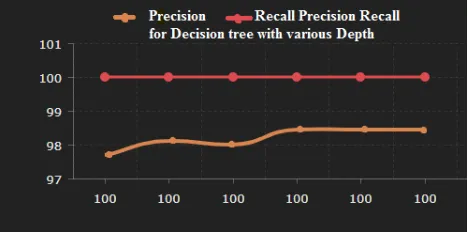
[image:3.612.44.278.313.429.2]
Fig. 1: Tree Depth vs. performance Decision tree
Decision Tree has various benefits over Naive Bayes. First, it chooses only one quality as analysis criteria at each node. Thus the method prioritizes the characteristic set,
Which performs a similar outcome as a weighted value function. Another, by defining the tree depth, it filters out characteristics that are less characteristic, hence prevent over fitting and defeating the unwanted noise of high-dimensional characteristic set.
Maximum tree depth is the key parameter in the Decision Tree algorithm and to select the optimal benefit test runs are conducted. Initial runs are transferred over the depths scale of 5 to 40 with a step of 5. The second repetition of runs uses a finer step, with the depth varying from 6 to 11.
Fig. 1 presents the course of precision and recalls for standard class with different tree depth. A Decision Tree classifier with maximum depth of 9 is chosen based on the issues, which gives the optimal combination of accuracy and recall.
By using the trained Decision Tree the classification of the interference matrix is given in Table III below.
TABLE III: Decision Tree Confusion Matrix
TruePositiveRate = 0.9652 FlasePositiveRate = 0.0918 FlaseNegativeRate = 0.0122 TrueNegitiveRate = 0.9082
C. K-means clustering formation
K-means clustering, as registered by its signature, and combinations provided data set a determined number of clusters according to their geometric sections in the location crossed by the characteristics.
This algorithm consists of the following steps:
1. Initialisation of the K cluster centroids (randomly) 2. Indicate every sample through the cluster whose centroid
is adjacent to the sample applying Eq. 9
3. Every cluster centroids are reset in the middle of all samples within the corresponding cluster using Eq.10
Analysis of test results is simply obtained by deciding the adjacent centroids based on Euclidean distance. This is seen that created clusters are not marked, while the test data requires being categorized as either attack or normal. Every centroid is attached to one of class 0 to 4 on the basis of a bulk vote of all samples in this cluster are added in a new step.Test data is then marked the related class as its adjacent centroid.
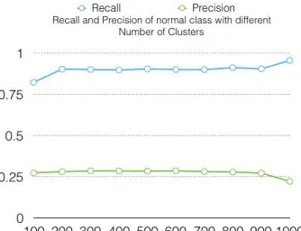
The data set is viewed in high dimensional space forming five clusters in the ideal condition. However, regarding the fact that each class can be additionally divided into different sub-classes, it is likely to have many extra clusters. Even two clusters of the same class may not be located next to others which indicates data is not linearly divisible .A number of cluster centroids need to choose wisely to address the issue. As a common practice, a character of centroids is fixed to a large amount in a direction to allot with data skew as well as that non-linear divisible dataset. But, an arbitrarily general K value may rise in over-fitting.
Fig. 2: Number of clusters and their K-means performance
[image:4.612.84.251.53.181.2]The 400-cluster model is chosen since it creates most adequate results in cross-validation. It is also recognized that the execution of this pattern is simple stable over various runs. But, no cluster of type 3 (R2L attack) can be defined steady for such a large K value. The confusion matrix is presented in Table IV which is obtained from a changed 400-cluster K-means algorithm.
TABLE IV: Confusion Matrix for K-means
TruePositiveRate = 0.937
FlasePositiveRate = 0.1005
FlaseNegativeRate = 0.0163
TrueNegitiveRate = 0.8995
D. Discussion
The confusion matrices for all three different stage classifiers show relevant results. It is regarded that although True Positive Rate is high (>90%), which overcomes the presence of the false signal. But, the False Positive Rate (FPR) is at high level. Which means reasonable protection risks resulting from undetected attacks?
A possible root reason for the poor production is that some attack traffic has characteristic feature response related to normal class while others may have related characteristic patterns. A single classifier qualified with the whole set is so biased towards the most distinct characteristics. In the next segment, multi-stage classifier designs are intended to defeat this condition.
5. MULTI-STAGE CLASSIFIER
The three single-stage algorithms give adequate recall value for the standard set. But, the almost low accuracy value means a high amount of undetected attacks. One of the viable reasons is that misclassified traffic has a related characteristic name linked to standard class. The purposed solution is to execute various classifiers that produce the accurate analysis. Two several methods are presented in this part. Casual growth creates identical classifiers while the Decision Tree with GMM model forms a cascaded classifier model.
A. Random Forest
A purest form of random forest is a set of Decision Trees. Every decision tree is trained independently with only a subset of training units. As a result, trees are created with various analysis standards at an individual level. The randomness assists to decrease the variance. An addressed test sample is thus arranged applying all various trees and the label is selected based on a bulk vote [8].
To define a number of decision trees in random forest algorithm, a common trade-off is there. An extended number of trees may develop the analysis execution, but, result in delayed runtime. A number of DTs from 10 to 15 are used to conduct test runs.The performance variation is not vital across several runs.
Therefore, the product of trees is defined to 11, which creates more stable returns over multiple test runs.
The result of analysis of confusion matrix using the Random Forest algorithm (RFA) is given in Table V.
TABLE V: Random Forest Confusion Matrix
TruePositiveRate = 0.99 FlasePositiveRate = 0.005 FlaseNegativeRate = 0.092 TrueNegitiveRate = 0.907
B. Decision Tree with Gaussian Mixture Model
The significant performance concern is the accuracy value of the standard class. Thus a cascaded classifier is offered where the second stage classifier simply acts upon the standard class specified by the first classifier. The second stage classifier is so trained to recognize a less variation within attack and normal class. Decision Tree is chosen as the first classifier as it presents the best execution out of the three algorithms in Section 3. Gaussian Mixture Model (GMM) is used to obtain the second stage classifier.
The test sample is allotted to the class that it most likely refers to. It is plain that GMM is an unsupervised training algorithm. GMM is able to manage non-linear frame in the data sets as K-means clustering.
GMM performs four sub-models, every equivalent to a modified covariance matrix. As among different training algorithms, test runs are handled to decide optimal parameter setting. Balanced covariance matrix produces the excellent result in cross-validation. The confusion matrix of an analysis result among the cascaded classifier is shown in Table VI.
TABLE VI: Cascade Confusion Matrix
TruePositiveRate = 0.937
FlasePositiveRate = 0.1005
FlaseNegativeRate = 0.0163
C. Discussion
It is mentioned that both multi-stage classifiers provide the limited production development. The further in-depth analysis in the dataset is triggered by the results. It is known that maximum misclassification issues from R2L attack (class 4) and U2R attack. (Class 3) A particular study shows the resulting insights.
A U2R attack produces a much short sample size in both learning set and test set compared to another class. Thus, the unusual characteristic pattern is not suitably determined by the classifiers.
In addition, a training set and test set does not support related configuration over various classes. Barely 0.25% of training individuals are of R2L attack type. But, there equal to 5.23% of them in the test set. The irregular pattern results in the preference of trained classifier, thus poor performance in knowing here dimmed class.
Finally, the R2L attack (class 4) can be the extra division into various sub-types of attacks. Considering the initial characteristic data shows that R2L attack (class 4) samples in the test set and R2L attack (class 4) samples in training set relate to various classes. It is much likely that these sub-classes must various characteristic patterns. Thus the trained classifier is not capable to classify the unknown pattern in the test set.
In result, an entire training set should be restored in order to develop the classifier with unusual performance.
6. CHARACTERISTIC REDUCTION
The optimal depth for the highest-operating Decision Tree-based classifier is 9, showing that there are irrelevant or unnecessary characteristics out of the 41-dimension characteristic space. Accordingly, the characteristic loss is used as a further optimization for the Intrusion Detection Systems with machine learning algorithm.
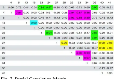
Fig. 3: Partial Correlation Matrix
The method for characteristic reduction is shown below: 1. Produce correlation matrix for entire characteristic set 2. Classify characteristic groups with unusual pair-wise
correlation
3. Utilize Principal Component Analysis to decrease the dimension of every characteristic group
An incomplete correlation matrix is given in Fig. 3 using Pearson coefficient in Eq.11 the correlation is computed and the group of features with high correlation are selected in highlighted fields as follows:
The new feature set is used to retrain the sordid line single stage classifiers. However, the performance improvement is peripheral. Detailed performance matching for all models in this document is displayed in the end.
[image:5.612.342.549.334.495.2]To analyze counter-intuitive result an extra analysis of feature correlation is needed, feature reduction is employed to individual classes of traffic in the outline by reapplying steps 1 &2 on a singular class of samples, the result given in Table VII.
TABLE VII: Individual class Feature correlation
Class Correlated Features
2 & 5 & 32 & 34 & 35 Probe 27 & 28 & 40 & 41
23 & 29 & 30
4 & 5 & 25 & 26 & 38 & 39 DoS 27 & 28 & 40 & 41
2 & 24 & 29 & 33 & 34 & 36
U2R 27 & 28 & 40 & 41 27 & 28 & 40 & 41 R2L 32 & 34 & 36
13 & 16, 26 & 26, 29 & 30
Various correlated groups are pointed in each class which has a unique feature signature/pattern.On the other hand, it unveils that the generic feature rebate approach is too competitive. It does help to consolidate tautological features. However, it combines some of the distinctive features from various classes as well. Therefore, a one-vs.-all classifier with class-specific feature reduction may give high-grade results. Due to time arrests, this approach is not performed. The concluding statements highlight this procedure as a future augmentation of this project.
7. CONCLUSION
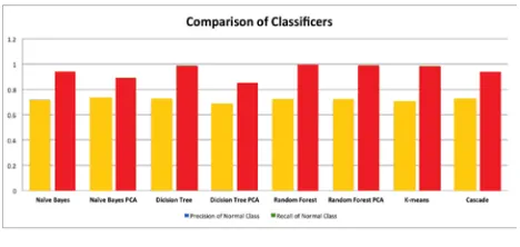
[image:5.612.37.267.503.663.2]Fig. 4: Comparison of Classifier
recall (true positive facing condition positive) as the target is to analyze network traffic into normal against intervention. The results record steady performance across different approaches. The values are recalled in the range 90% to 99% and high percentage as a low rate of false alarm. However, the accurate value ranges in between 70% to 75%, traversing to potential risks of undetected outbreaks.
In the further study root cause rests in the data sets.The different format of immature features, the pre-processing and normalization step cause anomalous patterns and the five classes are not evenly allocated in the training set. Data skew points to the bias in skilled classifier and thus deteriorated efficiency while analyzing test data. Each class consists of varied sub classes of similar feature signature/pattern are not positively hold by training and test data in the same class. Finally, features are correlated but the correlation pattern alters across distinct classes. Therefore PCA over complete training set does not better the achievement. In way of the high qualities essential to the dataset, later work should concentrate on producing customized data processing systems earlier to achieving extra complicated learning algorithms. Some proposed regulations are shortly presented here.
1. Examine the value combination of different characteristics to choose more proper normalization purpose
2. Re-Design training data set with an even dispersion over another class
3. Excellent categorization of the common attack
4. Behavior class-specific characteristic decrease accompanied by one-vs-all organization with the decreased characteristic
8. REFERENCES:
[1] KDDCup1999Data,http://kdd.ics.uci.edu/databases/kddcup99 /kddcup99.html, Web. Oct 2015.
[2] learning algorithms fail in misuse detection on KDD intrusion detection data set”, 403-415, 2004.
[3] Leonid Portnoy , Eleazar Eskin , Sal Stolfo,” Intrusion detection with unlabeled data using clustering “In Proceedings of ACM CSS Workshop on Data Mining Applied to Security
(DMSA-2001)” pp 5-6 Available at “http://citeseerx.ist.psu.edu/viewdoc/download?doi=10.1.1.126.
2131&rep=rep1&type=pdf”
[4] Adetunmbi, A.O., Alese, B.K., Ogundele, O.S and Falaki, S.O. (2007b). A Data Mining Approach to Network Intrusion Detection, Journal of Computer Science & Its Applications, Vol. 14 No. 2. Pp. 24 -37
[5] A. M. Chandrasekhar , K. Raghuveer, “Intrusion detection technique by using fuzzy neural network and svm classifiers, in “IEEE International Conference on Networking, Sensing and Control”, 2013, pp. 1-7.
[6] kdd-cup-99 Dataset, Available at” https://github.com/raja434/kdd-cup-99-spark”Mon.DEC2017”
[7] and argumentation methods in modern intelligent decision
support systems”
95.
[8] Strobl, C., Malley, J., & Tutz, G.” Rationale, application, and characteristics of classification and regression trees, bagging, and random forests. In Book Psychological Methods 14(4)”, pp 323-348.
AUTHOR DETAILS:
• Syamala Rao P. secured his Master of Technology (M.Tech.) in Information Technology degree from Andhra University. He is a topper in academics and secured gold medal in his M.Tech. He has 15+ years of experience in Academics and he is currently working as an Associate Professor in Information Technology department of Shri Vishnu Engineering College for Women. He worked as Head of Department, Master of Computer Applications in D.N.R. College, Bhimavaram.His research areas on Machine Learning, Artificial Intelligence and Mining.
• Dr. G. P. SaradhiVarma is Principal, S.R.K.R Engineering College having academic experience of 24 Years. He acted as editorial board member for different International/National journals. He has been recognized as Ph.D. Guide for Andhra University, Nagarjuna University, Jawaharlal Nehru Technological University, Krishna University and Produced 6 Ph.D. Thesis. He is handling research projects funded by AICTE and UGC