DOI: http://dx.doi.org/10.26483/ijarcs.v10i1.6367
Volume 10, No. 1, January-February 2019
International Journal of Advanced Research in Computer Science
RESEARCH PAPER
Available Online at www.ijarcs.info
ISSN No. 0976‐5697
FEATURES EXTRACTION IN 3D IMAGES VISUALIZED IN HEXAGONAL
LATTICE OF Z
3GRID
Mohd. Sherfuddin Khan
Research Scholar,Department of Electronics, G.H Raisoni College of Engineering, Nagpur,
Maharashtra, India
Vibha Bora
Professor & Head Electronics Dept. G.H Raisoni College of Engineering, Nagpur,
Maharashtra, India
Vijay H. Mankar Head of E&TC Government Polytechnic Ahmednagar, Maharashtra, India
Abstract: visualizing and processing Three Dimensional Digital images to Extract features in 3D images has become a subject of interest now-a days as many researchers are still processing and visualizing 3D digital images using 2.5D algorithms rather than 3D algorithms which is imprecise . and the implicit arrangement of human visual sensor array is hexagonal in nature .this intended many people including researchers and scientist for a long time to process the digital image over hexagonal prism lattice to extract better curvilinear features when compared to image processed over Rectangular lattice . in This paper we propose a simulated hexagonal prismatic lattice .and the hexagonal image Algebra for Extracting features processed on hexagonal prism lattice using algorithms developed in the framework of CLAP and 3D morphology . and real time 3D MRI images for testing the algorithms has been demonstrated along with sectioned view for visual inspection of linear and non linear features.
Keywords: Mathematical Morphology; Volumetric Features; Surface Detection; 3-D Image Processing
1. INTRODUCTION
Descriptionof an images in dissimilar scales and views applicable , to the need of the user is utmost significance and the present situation in visualization based systems. This will help the researchers to extract various features in directions which will then improve the division and segmentation of the images. In this juncture, Sima and Kay[1] put forward off-nadir parts which are given less importance and also not considered earlier. Such a way has provided efficient optimization in rendering. Rather than using the excess data, only the data which is near viewing imagery data is taken as input against those pixels with an maximizedgeometry for the process of rendering. This pixel which is maximized is further used as the pixel that corresponds to the to see angle that is most orthogonal that models the actual surface of the object[1].For efficient understanding of morphology of a three dimensional structure range images are required, which provide the basic necessity . An efficient edge detection algorithm must be able to extract features in such a way that they are linear in range as well as intensity of the image data. Most of the edge detection algorithms cannot detect edges appropriately in the presence of noise as they will be focusingon synthetic range images. Hence, Alshawabkeh[2] proposed an efficient edge detection algorithm which is mathematicallyefficient that can better localize edge pixels and is also robust to
that of the 2.5D. Features that are extracted from such a three dimensional visualization will help in divisionof three dimensional objects[7]. Peizhi Chen and Xin Li[8] presented a novel algorithm for volumetric images. The matching algorithm first extracts the features of the image using 3DSIFT. Such a featureis viewed to be scale and rotation invariant. Further, common features are processed using an improved spectral matching algorithm which has resulted in one to one mapping of these features. These features can be used for modeling of motions in medical images for processing and analysis. The major problemthat is posed by three dimensional imaging is the validation which may be either qualitative or quantitative. The former compares different visualization methods for a single task and latter gives the measure of the proposed techniques in terms of precision, accuracy and efficiency of the measurement[9]. Describing a three dimensional model is done by using meshes. Different features viz., volume, coefficients of more transformations, moments can be calculated from these meshes[12].The three dimensional descriptation can be secured by processing of the images using rectangular or hexagonal grid. For such a descriptation a coordinate system must have its basis vectors which are non-orthogonal [13]. many algorithms exist forextraction of edges from the images which are sampled using rectangular grid. One such algorithm is CLAP. It is identified that hexagonal sampling[15-16] provides better curvilinear visualization when compared to the rectangular grid based processing[14].It is observed that CLAP based surface detection algorithm takes less time for finding of the surface[17].we put forward a pseudo-hexagonal prismatic lattice. In this work we put forward a pseudo-hexagonal prismatic lattice based volumetric features detection and 3D morphology based surface detection on hexagonalized images . The processing of these images gives a of high quality that are defined on multi-dimensional grids. These are further used for getting an insight in to the scientific problem[20]. Section II) clearly outlines the problem definition, Section III) details the mathematical background of the proposed solution, Section IV) describes the proposed solution, Section V) Processing of 3D hexagonal images using 3D algorithms Section VI) provides the conclusion and future scope.
II PROBLEM DEFINITION
Creating hexagonal image Algebra for Processing and visualizing different MRI test images on Hexagonal prism lattice to Extract Features For Visual inspection and comparing with Rectangular grid based processing .
III )THE MATHEMATICAL BACKGROUND OF THE PROPOSED SOLUTION
Two major paradigms have been used in the development of 3D image processing algorithms. They are (i) Cellular Logic Array Processing (CLAP) and (ii) Mathematical
Morphology.
3.1 Cellular Logic Array Processing
The Algorithms used for processing 3D MRI images to extract features are developed in the fram work of cellular – logic arry processing and 3D Digital morphology . In this context, some basic mathematical preliminaries of cellular logic array processing are provided .
3.1.1 On the notion of Normal Algorithms
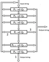
[image:2.612.386.488.357.486.2]the notion of normal algorithms are introduced In 1951, by Andrei Andreevich Markov (A. A. Markov) which are idealized realizations of sequential computing machines. A normal algorithm is an ordered list of substitution (production) formulas which fall under Chomsky’s type 0 grammar category. The functional attributes of a normal algorithm follow the attributes of a partial recursive function.
Fig. 1: Functional block diagram of a normal algorithm
Legend: Pi and Qi are words from an alphabet A and {,
N RAD Substitution Formulas
Formula Number
; A 1
Q 2
; E 3
Normal algorithms can be constructed over union of various alphabets. The principle of normalization of algorithms states that there is no algorithm ever constructed or going to be constructed in future which is non-normalizable.
3.2.1 On the notion of Cellular Automata
Sthanislaw Ulam and von Neuman in 1936 introduced cellular automata and it was known as tessellation automaton. Cellular automata are idealized parallel processing computing systems. A cellular automaton is an
[image:3.612.63.286.78.184.2]array of cells called sites. Each cell takes on values from a set of numbers N = {0, 1, 2, …, N-1} at a particular instant of time. Each cell value is computed by an updating rule that involves values of certain neighbourhood R of cells. An updating rule condition is simultaneously parallely applied to all cells in the array at a particular instant of time and values for next instant of time calculated. This amounts to saying that a cellular automaton is a parallel processing system each cell being treated as a processor. The family of cellular automata is denoted as DNRCA, where D refers to the dimension, N refers to the number of values a cell can take and R refers to the neighbourhood. For example 123CA refers to the family of one dimensional binary valued three neighbourhood cellular automata with 256 updating rules called linear Boolean functions. This means that one can construct 256 one dimensional cellular automata belonging to the category 123CA.
Figure 2 shows an unbounded linear array of 123CA category of cellular automata.
--- i-4 i-3 i-2 i-1 i I+1 I+2 I+3 I+4 ---
Fig. 2: Linear array of 123CA cellular automata family The site values of all cells of a cellular automaton belonging to the family123CA at time instant t is shown in figure.3
--- (t)
i-1 (t)
i-1 (t)
i-1 (t)
i-1 (t)
i (t)
i+1 (t)
i+2 (t)
i+3 (t)
i+4 --- Fig. 3: Site values of 123CA based cellular automaton
Now an updating rule is applied to all cells at a time. Considering the ith cell and its three neighbourhood cells (a cell is neighbour to itself) an updating rule would be of the form (t+1)i = ((t)i-1 , (t)i , (t)i+1), where (t+1)i is the updated value of the ith cell by the formula . As mentioned earlier, once can construct 256 linear Boolean functions 0, 1, 2, ---, 255.
IV) PROPOSED SOLUTION
4.1 3 D Image Visualization in Hexagonal Prism
Lattice of Z3 Grid
Brief Explanation of Hexagonal lattice in Z3
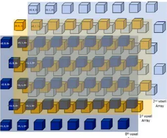
A voxel in a 3D lattice is shown in figure 4(a). Fig.4(b) which is a 10x10x10 array of voxels. Each voxel is shown by a gray tone or a color in terms of R, G and B values . If R, G and B values are identical then the voxel is said to be gray level voxel.
[image:3.612.366.508.550.711.2]
Fig. 4: Voxel in a 3D lattice and 10x10x10 array of voxels
The relation between voxels of rectangular lattice then that of simulated hexagonal lattice interlinked with the
formulas: as (i) in the hexagonal lattice of kth voxel array in the even row element is linked to rectangular lattice as (Note: 0th row is even row), <kx
i, kyj, kzk> = <Nx2i, Ny2j, Nz2k>, and (ii) in the hexagonal lattice of k
th
[image:4.612.91.260.165.305.2]voxel array in the odd row element is linked to rectangular lattice as <kxi, kyj, kzk,> = <Nx2i, Ny2j+1, Nz2k 22-23].
Fig. 6: Hexagonal lattice points depicted in Z3 grid
Figure. 7: Sample image displayed on rectangular and hexagonal lattice in Z3 grid
The objective of this paper is to Extract volumetric and superficial features of various components in a 3D hexagonalized image using algorithms developed in the frame work of i) cellular logic array processing and ii)3D digital morphology and compare with the rectangular grid processed images for visual inspection .
V) PROCESSING OF 3D HEXAGONAL IMAGES USING 3D ALGORITHMS
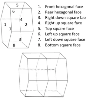
5.1 Three dimensional structuring elements in 3D Hexagonal Prism Lattice of Z3 Grid
Front Plane (K-1) Central Plane (K) Rear Plane (K+1)
Figure 8: 21- Neighbourhood Structure
the 21-neighborhood structure contain a total of 324 convex polyhedrons (prisms) which are in the 21-neighborhood structure in to seven groups in which 25 are basic convex structuring elements which are listed below as .
Group A: No voxel is eliminated we get 1 combinationA = {1,2,3,4,5,6,15, 16,17,18,19,20}
Group B: Eliminating one voxel we obtain 12 combinations
B1 = {2,3,4,5,6,15,16,17,18,19,20}; B2 = {1,3,4,5,6,15,16,17,18,19,20}; B3 = {1,2,4,5,6,15,16,17,18,19,20}; B4 = {1,2,3,5,6,15,16,17,18,19,20}; B5 = {1,2,3,4,6,15,16,17,18,19,20}; B6 = {1,2,3,4,5,15,16,17,18,19,20}; B15 = {1,2,3,4,5,6,16,17,18,19,20}; B16 = {1,2,3,4,5,6,15,17,18,19,20}; B17 = {1,2,3,4,5,6,15,16,18,19,20}; B18 = {1,2,3,4,5,6,15,16,17,19,20}; B19 = {1,2,3,4,5,6,15,16,17,18,20}; B20 = {1,2,3,4,5,6,15,16,17,18,19};
Similarly one can construct hexagonal polyhedrons (prisms) by removing various corner voxels in a combinatorial manner.
Group C D E F G : Eliminating two ,three, four , five, six voxels we obtain 54 ,112 ,105 , 36 ,4 combinations Basis Polyhedrons from E and F and G Groups
E1, 4, 15,18; E1, 4, 16,19; E1, 4, 17,20; E2, 5, 15,18; E2, 5, 16,19; E2, 5, 17,20; E3, 6, 15,18; E3, 6, 16,19; E3, 6, 17,20,F1, 4, 15,17,19; F1, 4, 16,18,20; F2, 5, 15,17,19; F2, 5, 16,18,20; F2, 5, 15,17,19; F2, 5, 15,17,19; F1, 3, 5,15,18; F1, 3, 5,16,19; F1, 3, 5,17,20; F2, 4, 6,F2, 4, 6,16,19,F2, 4, 6,17,20 G1,3,5,15,17,19 ; G1,3,5,16,18,20 ; G2,4,6,15,17,19 ; G2,4,6,16,18,20
The above mentioned 324 convex –polyhydrons are used as structuring elements for processing hexagonalized 3D images to extract features but the basic 25 structuring elements do the job of all as they are basic pattern.
Sl. No Convex Hexagonal Polyhedron (Prism) Remarks 1 2 3 4 5 6
E1, 4, 15,18 E1, 4, 16,19 E1, 4, 17,20 E2, 5, 15,18 E2, 5, 16,19 E2, 5, 17,20
4 corners removed
7 8 9
E3, 6, 15,18 E3, 6, 16,19 E3, 6, 17,20 10 11 12 13 14 15 16 17 18 19
F1, 4, 15,17,19 F1, 4, 16,18,20 F2, 5, 15,17,19 F2, 5, 16,18,20 F2, 5, 15,17,19 F2, 5, 15,17,19 F1, 3, 5,15,18 F1, 3, 5,16,19 F1, 3, 5,17,20 F2, 4, 6,15,18
20 21
F2, 4, 6,16,19 F2, 4, 6,17,20
22 23 24 25
G1,3,5,15,17,19 G1,3,5,16,18,20 G2,4,6,15,17,19 G2,4,6,16,18,20
[image:5.612.55.296.53.134.2]6 corners removed
Table .1 Basis hexagonal polyhedrons.
5.1.1 Volumetric Features Extracted in 3D images using CLAP algorithms
Extracting 3D volumetric features can be done by scanning the 3D image with 3D scanning window and processing it with the algorithm meant for it and clap based volumetric feature extraction is explained in [19][20]. For visual inspections Some test images are processed and features are extracted using clap algorithm are shown below .figures 10 shows Some the images on Rectangular and hexagonal grids for visual inspection.
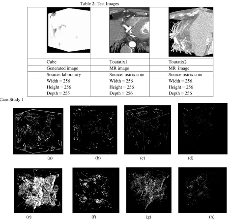
Table 2: Test Images
Cube Toutatix1 Toutatix2
Generated image MR image MR image
Source: laboratory Source: osirix.com Source:osirix.com Width = 256
Height = 256 Depth = 255
Width = 256 Height = 256 Depth = 256
Width = 256 Height = 256 Depth = 256 Case Study 1
(a) (b) (c) (d)
(e) (f) (g) (h)
Figure 9 .1 (a)3D edge detected toutatix1 (b) Sections from 40th slice to 100t slice (c) 3D edge detected hexagonalized toutatix1 (d)Sections from 40th slice to 100th slice
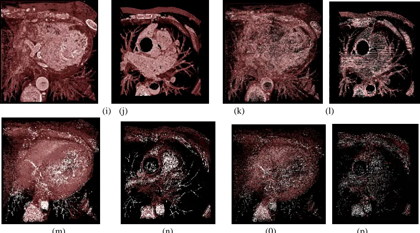
[image:5.612.61.529.187.640.2](i) (j) (k) (l)
[image:6.612.92.520.54.291.2]
(m) (n) (0) (p) Figure 9 .2 (i) 3D edge detected toutatix1 (j) Sections from 40th slice to 100t slice (k) 3D edge detected hexagonalized toutatix1 (l)Sections from 40th slice to 100th slice
(m) 3D skeletonized toutatix1 (n)Sections from 40th slice to 100thslice (0) 3D skeletonised hexagonalized toutatix1 (p) Sections from 40th slice to 100th slice
(q) (r) (s) (t)
[image:6.612.91.524.359.581.2]
(u) (v) (w) (x) Figure .9.3 (q) 3Dedge detected toutatix2 (r) Sections from 40th slice to 100t slice (S) 3D edge detected hexagonalized toutatix2 (t)Sections from 40th slice to 100th slice
(u) 3D skeletonized toutatix2 (v)Sections from 40th slice to 100th slice (w) 3D skeletonised hexagonalized toutatix2 (x) Sections from 40th slice to 100th slice
Figure. 9 shows Edge and skeletonised MRI images processed over Rectangular and hexagonal Grids for visual inspection
Table 3: processing Times Image Edge Skeleton Toutatix1 11 sec 399.44sec toutatix2 11.42sec 409.51 sec
5.1.2 Mathematical Morphology in a 3D Hexagonal Prism Lattice of Z3 Grid
The 3D mathematical operations in a 3D Hexagonal Prism Lattice of Z3 Grid are performed by convolving the
3D Structuring Element B on the Original image X. The Dilation and Erosion is given by the equations (1)&(2)
X θ B = max (Xx+i, y+j, z+k )
(i,j,k) ∈ B………..(1)
X θ B = min (Xx+ i, y+ j, z+k ) (i,j,k) ∈ B ……….(2)
CASE STUDY : 2
(a) (b) (c) (d) Figure 10.1 (a) Cube dilated (b) Cube dilated sectioned from 40th slice to -100 slice
3D dilated form of Hexagonalized cube(f): Sections from 40th slice to 100th slice
(e) (f) (g) (h)
Figure 10.2 3D (e) Cube eroded forms (f) Cube eroided sectioned from 40 to -100 slice (g) 3D eroded form of Hexagonalized (h) cube eroided Sections from 40th slice to 100th slice
(i) (j) (k) (l)
Figure 10.3 (i) 3D dilated forms of toutatix1 (j): Sections from 40th slice to 100th slice (k)3D dilated forms hexagonalized toutatix1(l): Sections from 40th slice to 100th slice
[image:7.612.68.515.66.681.2]
(m) (n) (o) (p) Figure 10.4 (m) eroded forms of toutatix1 (n): Sections from 40th slice to 100th slice
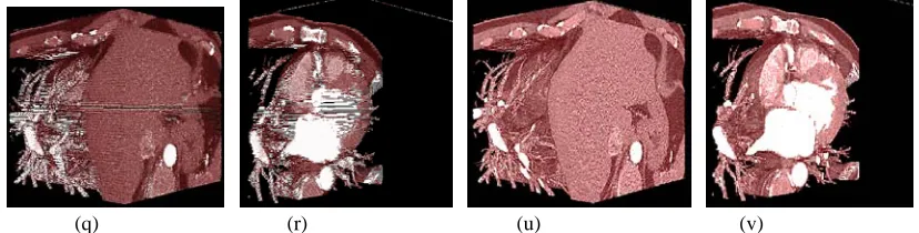
(q) (r) (u) (v)
Figure 10.5 (q)3D dilated forms of toutatix2 (r): Sections from 40th slice to 100th slice (u) 3D dilated forms of hexagonalized toutatix2 (v): Sections from 40th slice to 100th slice
[image:8.612.93.517.197.297.2]
(w) (x) (y) (z) Figure 10.6 (w) 3D eroded forms of toutatix2 (x): Sections from 40th slice to 100th slice (y) 3D eroded forms of hexagonalized toutatix2 (z): Sections from 40th slice to 100th slice
Figure. 10 shows Dilated and Eroded MRI images on Rectangular and hexagonal Grids for visual inspection.
Table 4: processing Times
Image Dilation Erosion
Toutatix1 8 sec 10sec toutatix2 8 sec 10 sec
Table 4 :gives the information regarding the time taken for dilation and erosion of standard test images Toutatix1 and Toutatix2 (Note: complex city remains similar whether it is rectangular or hexagonalized processed images )
5.1.3. Surface Detection in 3D Hexagonal Images Using Morphological Filters
For non-invasive type of medical surgeries the visualization algorithms will be of great help and The surface detection and visualization must be good enough such that the doctor can easily make a note of the presence of pathologies and polyps .Surface detection and visualization on different grids has become much important as layered wise analysis is playing much important role in radiology as surface detection using morphology gives layered wise visualization [21]. Surface detection of some standard 3D MRI images using morphological operations with sectioned view for visualization is shown below in figure 11. which tells the quality of image processed and visualized on different grids.
Case Study 3:
[image:8.612.69.510.570.682.2]
(e) (f) (g) (h)
Figure 11 (e): 3D surface detected toutatix1 image (f): Sections from 40th slice to 100th slice (g): 3D surface detected hexagonalized toutatix1 (h): Sections from 40th slice to 100th slice
. (i) (j) (k) (l) Figure 11.(i): 3D surface detected toutatix2 image (j): Sections from 40th slice to 100th slice
[image:9.612.92.519.49.322.2](k) 3D surface detected hexagonalized toutatix2 l): Sections from 40th slice to 100th slice
Figure. 11 shows surface detected MRI images processed on Rectangular and hexagonal Grids for visual inspection
VI) CONCLUSIONS
Features extracted on hexagonal prism lattice (z3) grid with some standard real time 3D MRI images for testing the algorithm has been demonstrated along with sectioned view for visual inspection purpose of linear and non linear features is presented in this paper on different grids . Results shown provide visual proof of quality of algorithms used for processing images on rectangular and hexagonal Grids developed in the framework of ‘CLAP’. and by visual inspection of sectioned slices from 40th to 100 th slices of hexagonal processed slices we can notify that we are able to Extract curvilinear features in 3D images at the loss of information due to images processed on simulated hexagonal grid . to overcome that we have to acquire images on hexagonal monitor instead of rectangular or else we have to go for 3D compression of the image processed on simulated hexagonal lattice to get the effect of rectangular grid processed image which will be the next research scope of the work done.
VII) REFERENCES
[1] Sima, A. A. and Kay, S. (2007). Optimizing the use of digital airborne images for 2.5D visualization. In Abstract book of 27th Earsel Symposium, page 185, Bolzano, Italy.
[2] Y. Alshawabkeh, N. Haala, and D. Fritsch, “Range image segmentation using the numerical description of the mean curvature values,” in The International Archives of Photogrammetry, Remote Sensing and
Spatial Information Sciences. ISPRS Congress, 2008, p. 533.
[3] Cin-Young Lee and Erik K. Antonsson, "Surface Reconstruction of Etched Contours", International Conference on Modeling and Simulation of Microsystems, Cambridge, MA, U.S.A., April 1999. [4] Khromov D, Mestetskiy L. 3D Skeletonization as an
Optimization Problem; Proc. Canadian Conf. Computational Geometry; 2012. pp. 259–264.
[5] Akca, D., “A New Algorithm for {3D} Surface Matching”, Int. Archives of Photogrammetry, Remote Sensing and Spatial Information Sciences, 2004, 960-965.
[6] Haker, S., Angenent, S., Tannenbaum, A., and Kikinis, R., "Nondistorting flattening maps and the 3D visualization of colon CT images", IEEE Trans. of Medical Imaging, 2000.
[7] T. Hlavaty and V. Skala, “A Survey of Methods for 3D Model Feature Extraction,” Seminar on Geometry and Graphics in Teaching Contemporary Engineer.
[8] Chen, P., Li, X.: ‘Effective volumetric feature modeling and coarse correspondence via improved 3dsift and spectral matching’, Math. Probl. Eng., 2014, 2014, pp. 1–10.
[9] Udupa J K 1999 Three-dimensional visualization and analysis methodologies: a current perspective Radiographics, 19: 783–806.
[10] Brannon R M 2004: Curvilinear Analysis in a Euclidean Space. University of New Mexico.
[image:9.612.106.507.58.165.2]Soft Computing Approaches", International Journal of Recent Trends in Engineering, Vol. 1, No. 2, PP.250-254, May 2009.
[12] Zhang C, Chen T, “Efficient feature extraction for 2D/3D objects in mesh representation”, IEEE international conference on image processing, 2001. [13] W. E. Snyder, H. Qi, and W. A. Sander, “A coordinate
system for hexagonal pixels,” Med. Imag., vol. Pt. 1–2, pp. 716–727, 1999.
[14] M. Senthilanyaki, S. Veni, K. A. N. Kutty, “Hexagonal Pixel Grid Modeling for Edge Detection and Design of Cellular Architecture for Binary Image Skeletonization,” Annual India Conference (INIDCON), 1-6, 2006.
[15] S. Veni and Narayanankutty, K. A., “Image enhancement of medical images using gabor filter bank on hexagonal sampled grids”, World Academy of Science, Engineering and Technology, no. 65, pp. 816-821, 2010.
[16] Liu, Shih-chun, Laura H. Derick, and Jiri Palek., “Visualization of the hexagonal lattice in the erythrocyte membrane skeleton”, The Journal of Cell Biology 104.3, 1987, pp. 527-536.
[17] Chandra, G. Ramesh, et al. "EDGE Detection in 3D images using Cellular Logic Array Processing." Systems, Man and Cybernetics (SMC), 2014 IEEE International Conference on. IEEE, 2014.
[18] Elvins, T. Todd. "A survey of algorithms for volume visualization." ACM Siggraph Computer Graphics 26.3 (1992): 194-.
[19] Cullip U., Neumann U.: Accelerating Volume Reconstruction with 3D Texture Hardware. UNC Tech Report TR93-0027. (1993).
[20] Cabral B, Cam N and Foran J: Accelerated volume rendering and tomographic reconstruction using texture mapping hardware. VVS ‘94: Proc. 1994 Symp. on Volume Visualization (Tysons Corner, VA) (New York: ACM Press)
[21] Klaus Mueller, Fang Xu, and Neophytos Neophytou: Why do Commodity Graphics Hardware Boards (GPUs) work so well for acceleration of Computed Tomography?. SPIE Electronic Imaging 2007, Computational Imaging V Keynote
[22] Mihai Popescu.et.al “Graph-Based Volumetric Data Segmentation on a Hexagonal-Prismatic Lattice ”Proceedings of the Federated Conference on Computer Science and Information Systems pp: 745– 749 ISBN :978-83-60810-51-4