A COMPARATIVE STUDY OF CONVOLUTIONAL NEURAL NETWORKS FOR SEGMENTATION AND CLASSIFICATION OF REMOTE SENSING IMAGES

DOI: http://dx.doi.org/10.26483/ijarcs.v8i8.4764

Volume 8, No. 8, September-October 2017

International Journal of Advanced Research in Computer Science

RESEARCH PAPER

Available Online at www.ijarcs.info

ISSN No. 0976-5697

A COMPARATIVE STUDY OF CONVOLUTIONAL NEURAL NETWORKS FOR

SEGMENTATION AND CLASSIFICATION OF REMOTE SENSING IMAGES

Mrs. P.Dolphin Devi

Department of computer science GTN Arts College (Autonomous)

Dindigul,India

Dr K.Chitra

Department of computer science Government Arts College

Madurai, India

Abstract: Geographical satellite images that are used for the analysis of environmental and geographical plains are obtained through remote sensing techniques. The raw images collected from the satellites are not well suited for statistical analysis and accurate report preparation. So, the raw images undergo the usual image processing procedure such as preprocessing, segmentation, feature extraction and classification. Traditional image classification techniques have several spatial and spectral resolution issues. A novel image classification technique, namely, Convolutional Neural Networks (CNN) technique is an emerging research criterion. It is an extension of neural networks and deep learning approaches. In this paper, several CNN based image classification techniques are analyzed and their performance is compared. The techniques involved in this analysis include Full Convolutional Network (FCN), Patch-based classification, pixel-to-pixel based segmentation and convnet-based feature extraction. Each technique utilized different datasets for its own performance evaluation. Finally, the performance evaluations are analyzed in terms of accuracy.

Keywords: Remote sensing, Full Convolutional Network (FCN), Patch-based classification, pixel-to-pixel based segmentation, convnet-based feature extraction.

I. INTRODUCTION

Remote sensing is the process of monitoring a remote object without having a physical contact with that object. In general, the objects are observed by gathering data using the artificial satellites that are launched to revolve around the earth. Remote sensing technology has its wide applications in weather forecasting, agriculture, studies regarding the environment and hazards, fossil fuel and minerals identification, mapping of the land usage, and so on. During the analysis of disaster recovery and management, it is necessary for the government to collect the land cover for identifying the affected areas. The constellation satellites generate the high quality images of the entire earth in a less amount of time. The images produced by the geographical satellites have a large amount of noise and irrelevant data due to the distractions caused in the space. Remote sensing is regularly portrayed by complex information properties as heterogeneity and class irregularity, and covering class-contingent appropriations. Together, these perspectives constitute serious difficulties for making land cover maps or distinguishing and restricting items, creating a high level of vulnerability in acquired outcomes, notwithstanding for the best performing models. There is an immense research on characterization approaches that consider the range of each individual pixel to allocate it to a specific class. On the otherhand, more propelled systems join data from a couple neighboring pixels to upgrade the classifiers' execution, regularly mentioned to as spectral-spatial order. These methodologies depend on the separate distinctive classes in light of the range of a single pixel or of some neighboring pixels. In an extensive scale setting, these methodologies are not powerful.

Convolutional neural systems (convnets) have empowered huge achievements in different picture order errands and remote detecting picture order is not a specialcase to this pattern. Generally, neural systems have been viewed as secret elements and prepared end-to-end for aparticular grouping assignment. This has been one of the

purposes behind their prosperity, and the classifiers are found out in a manner that the most discriminative elements are utilized for characterization. In remote detecting, information marking is costly and substantial named datasets are rare. Two outcomes have made conceivable to evade the need of preparing information and disturbed the adjustment in context on convnets. The first is the perception that the yields of a neural system with irregular weights that can be used to prepare a classifier, which will bring about great accuracy in results. The second one is an intriguing property of convnets that it is conceivable to acquire exact result on a given errand by utilizing a totally inconsequential errand. The last layer for the job is also completed using the convnets and also effectively utilized as a part of remote detecting picture grouping. As an outcome of the above discoveries, the convent consists of two sections such as a component extraction part and a classifier part. This division is free and there is no strict lead which layers of the system includes extraction and classifier parts.

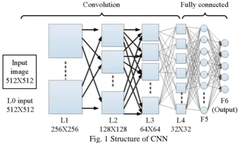
Fig. 1 Structure of CNN

provided to do a basic operation using which a single output is generated. The vector is used to provide the input to the system. The parameters of the function in the neural network include the weight vectors and the biases. The values of these parameters are identified using the training process. The remaining sections of the paper are organized as follows: Section II gives a brief note about FCN. Section III explains the patch-based classification and pixel-to-pixel based segmentation. Section IV describes convent based feature extraction. The performance of the all the techniques are analyzed in Section V and the paper is concluded in Section VI.

II. FULLY CONVOLUTIONAL NETWORK (FCN)

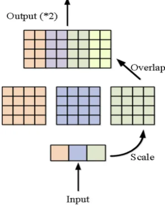
The FCN architecture[1]is proposed to generate dense predictions. The fully connected layer is converted to a convolutional layer. The dimension of the convolution kernel is to be chosen to coincide with the preceding layer. Hence, its connections are equal to a fully connected layer. The FCN architecture includes a deconvolutional layer for improving the resolution of the output feature map. It performs upsampling of the feature maps. The upsampled feature map comprises a central portion estimated by adding the input of two neighboring kernels. The upsampling is attained by the interpolation from a set of nearby points. The interpolation is parameterized by a kernel. The kernels should be large enough to overlap in the output, for the effective interpolation. The kernel states the level and extent of contribution from a pixel value to the neighboring positions, based on their locations only. The kernel values are multiplied by each input and the overlapping responses in the output are added to perform the interpolation.

Fig.2 depicts the deconvolution layer for 2× upsampling. The scaling step is performed based on the constant4×4 kernel. The interpolation kernel is an additional group of learnable network parameters irrespectiveofbeingdefined as apriori. Only one kernel contributes to the outer border that is an extrapolation of the input. The inner region is the interpolation. The extrapolated border is collected from the output to avoid artifacts.

The advantages of FCN over the patch-based approach are 1) Removal of discontinuities due to the patch borders. 2) High accuracy due to the simplified learning process and a smaller number of parameters.

3) Lower execution time due to the fast execution of convolution operations.

Fig.2 Deconvolution layer for 2× upsampling

Fig. 3(a) depicts the patch-based network architecture. The FCN is created by the convolutionalization of the existing patch-based network architecture. An existing framework is selected to benefit from a complete architecture and enable thorough comparison. Fig. 3(b) shows the FCN. Let us assumethat the size of output patch of the network is 1×1. Thus, a single output centered in its receptive field is dedicated. Next, the fully connected layer is transformed as a convolutional layer with a single feature map and spatial dimensions of the previous layer (9×9). Finally, a deconvolutional layer is added for upsampling the input by a factor of 4 to recover the input resolution. The original network can obtain the input images of different sizes.Inthe training stage, a 16×16 patch is obtained as output for matching the learning process in the patch-based network.

Fig. 3(a) Patch-based network and (b) Fully convolutional CNN architectures

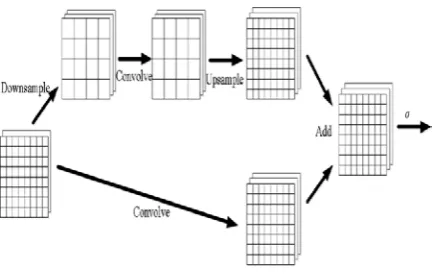
excluded extrapolation is denoted in white. Fig. 4 shows the two-scale convolutional module.

Fig. 4 Two-scale convolutional module

III. PATCH-BASED PIXEL CLASSIFICATION AND PIXEL-TO

-PIXEL SEGMENTATION

A. Patch-based classification

A Convolutional Neural Network (CNN) is trained on same image patches that are extracted from large training images [2]. Paisitkriangkrai et al. [3] achieved best accuracy

using patches. But, the image patch should be

classified according to the center pixel in order to choose a pixel shape. During the test-phase, the trained CNN is used for the efficient classification of whole test image.

• Patch-based CNN Architecture:

It involves four convolutional layers and two fully connected layers. The convolutionallayersinclude 32, 64, 96, 128 kernels of size 5×5×5, 5×5×32, 5×5×64 and 5×5×96, respectively.A stride of1on the 65×65×5 input image is applied on the kernels. A patch for every object is extracted initially with the object being centered for generating the training and validation data. Then, each patch is rotated randomly several times at various angles to generate additional training data for the object class. Further classes are sampled from the images, such that the center pixel belongs to the class of interest. The same amount of training data is sampled from each class to achieve class balance.To ensure efficient classification of larger images, the fully connected layers are converted to the convolutional layers. This reduces the computational complexity of the sliding window approach, where overlapping regions lead to the redundant computations, and allows the classification of various image sizes.

B. Pixel-to-Pixel segmentation

Apixel-to-pixel architecture is designed based on the FCN architecture [4]trained by using the cross-entropy loss function. This function is estimated by adding all the pixels in the image. But, it does not suit well for the imbalanced classes.The network is trained in small batches on the 256×256 pixel patches. The size of the patch is selected based on the Graphics Processing Unit (GPU) memory considerations [2].

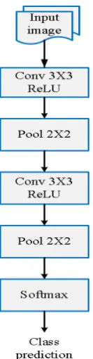
Fig.5 presents the pixel-to-pixel architecture that enables end-to-end learning of the pixel-to-pixel semantic segmentation. Itcontainsfour sets of double 3×3 convolutions. Each set is separated by a 2×2 max pooling

layer with the stride 2. The first convolutional layer has a stride of 2. All other convolution layers have a stride 1. The final 3×3 convolutionconsists of one kernel for each class to produce class scores. It is followed by a 1×1 convolution.Thefractional-strided convolution layer follows the convolutional layers. It learns to upsample the prediction back to the size of the original image and a softmax layer. The image patches are obtained from the input image with the overlap rate of about 50%. The patches are flipped left to right and up and down and rotated at 90 degree intervals, to yield eight augmentations per overlapping image patch.

Fig. 5 Pixel-to-pixel architecture

Two FCN models are trained to consider the imbalanced classes into account. In one FCN model, the weighting of the loss of the classes is performed using the median frequency balancing [5, 6]. This weighting process is performed depending on the ratio of median and actual class frequency in the training set.Other FCN model uses the standard cross-entropy loss. The modified cross-entropy function is calculatedas

(1)

Where denotes the weight of the class ‘c’, indicates the frequency of pixels in the class ‘c’, ‘N’ represents the number of samples in a mini-batch, ‘C’ denotes the set of all

classes, signifies the softmax probability of sample ‘n’ in the class ‘c’ and represents the label of the sample ‘n’ for the class ‘c’. The is calculated as

(2)

IV. CONVNETS

learning rate is not reduced for eight epochs. The learning is terminated if the validation error did not drop for 30 consecutive epochs or if the learning rate was reduced by a factor of more than 1000 in total.The features are analyzed further using Fisher criterion to obtain better insight behind the classification accuracy and evaluate the separability of classes in the feature space. Fisher criterion is used for evaluating the ability of Gabor-based features for the discrimination between two textures. A cluster is formed in the feature space using the feature vectors for images from a single class. The features are more suitable for discrimination between the classes, if the separability of the clusters is better. The separability depends on the distance and compactness between the clusters. It can be assessed using Fisher discriminant analysis.

Fig. 6 Convnet with two convolutional layers and without fully connected layers

If a set of d-dimensional samples belongs to the ‘c’ class, the Fisher discriminant analysis finds the

projections to (c-1) dimensional space where

. denotes the projection

matrixobtained by increasing the Fisher criterion. The Fisher criterion is the proportion of the within and between class scatter of the projected samples . The between-class scatter matrix is calculated as

(3)

Where denotes the number of samples in the ith class and m indicates the mean vector of all samples.

(4)

is the mean vector of the set of feature vectors from the ith class, . The between-class scatter matrix is a measure of the distance between the clusters and within-class scatter matrix is a measure of compactness between the clusters. It is defined as

(5) The total scatter matrix is defined as

(6)

The criterion function has the following form

(7) Where represents the trace of a matrix, which is the sum of the Eigen values of the matrix. If the equation (7) is increased, there is an increase in the between-class scatter and decrease in the within-class scatter. This is equal to the increase in the distance and compactness between the classes. If the Fisher criterion value is large, the separability of the classes is better. A Distribution Separability Criterion (DSC) is used to measure the discriminative power of features. It is computed as

(8)

Where denotes the mean of the distance between means and indicates the mean of the standard deviation of the class conditional distributions. The DSC is similar to the Fisher criterion in the two-class case.

V. PERFORMANCE ANALYSIS

The FCN is built and its performance is evaluated using the Massachusetts Buildings dataset. This dataset is derived by correcting the minor errors of OSM frozen dataset. It consists of images captured from Boston whose spatial resolution is 1 square meter. It included certain area for validation, training and testing. The validation area ranges around 9 square kilometer, 340 square kilometer for training and 22.5 square kilometer for testing. These color images are grouped under two categories, namely, building class and not building class respectively. The FCN is analyzed using three metrics including accuracy, AUC, and IoU. The fine tuning is done by adjusting the weights of the images in the OSM Forez dataset. The accuracy of FCN is 99.126, whereas the accuracy of FCN after fine tuning is 99.459. The AUC and IoU of FCN is 0.969166 and 0.48 respectively, whereas the AUC and IoU of the fine-tuned FCN is 0.99699 and 0.66 respectively.

For evaluating the patch-based classification and the pixel-to-pixel segmentation, a dataset namely, ISPRS Vaihingen 2D semantic labeling contest dataset is utilized. This dataset possess varied sized images of 33 numbers in which each image has 3 million to 10 million pixels. This dataset contains the images captured in Vaihingen located at Germany using high quality true ortho photo from a distance of 9 cm from the object. Each image contains a Digital Surface Model (DSM) apart from True Ortho Photo. To overcome the issues that occur due to varied ground height, extra DSM also included in the dataset. There are 16 ground truth images out of 33 images.Two metrics such as accuracy and F-measure are used to measure the performance of patch-based classification and pixel-to-pixel segmentation. The patch-based classification misclassifies some small plants as the area of vegetation. Its classification accuracy is high for buildings and roads. When compared to patch-based classification, pixel-to-pixel patch-based segmentation achieved higher accuracy. The classification accuracy of patch-based method, in the case of buildings is 94.04%.

dataset includes four types of classes such as grassland, roads, barren land, buildings and water bodies. The classes in the SAT-6 dataset are classified as water bodies, roads, barren land, grassland, trees, buildings and water bodies.

As the feature extraction plays a vital role in improving the classification accuracy, the convnet based feature

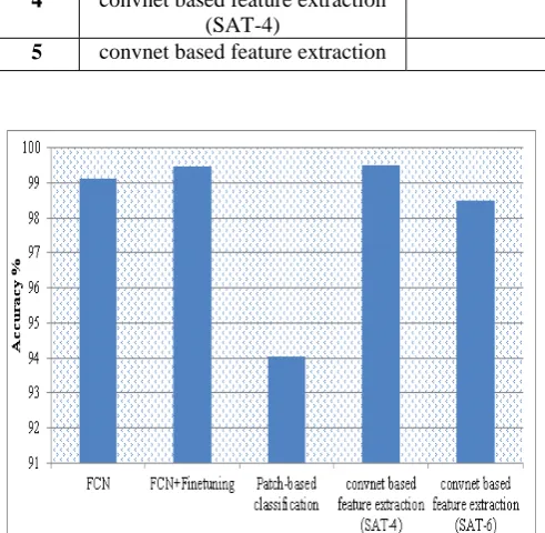
technique is analyzed by varying the number of convolutional layers. The highest accuracy attained using SAT-4 dataset is 99.52% and SAT-6 data is 98.51%. The accuracy analysis of the methods is presented in Table I and its graphical plot is represented in Fig.7.

Table I. Accuracy analysis of various remote sensing image classification techniques

S. No. Technique Dataset Used Accuracy

1 FCN Massachusetts Buildings dataset 99.126

2 FCN+Finetuning OSM Forzen dataset 99.459

3 Patch-based classification ISPRS Vaihingen 2D semantic labeling contest dataset 94.04

4 convnet based feature extraction (SAT-4)

SAT-4 dataset 99.52

5 convnet based feature extraction SAT-6 dataset 98.51

Fig. 7 Accuracy graph of remote sensing image classification techniques

VI. CONCLUSION

In this paper, several geographical image classification techniques based on CNN is studied and analyzed. The techniques are FCN, Patch-based classification, pixel-to-pixel based segmentation and convnet-based feature extraction. The FCN and fine-tuned FCN utilized MassachusettsBuildings dataset and OSM Forzen dataset respectively. ISPRS Vaihingen 2D semantic labeling contest dataset is used to evaluate the performance of patch-based classification technique. The convnet based feature extraction technique is analyzed using two datasets such as SAT-4 and SAT-6. All the techniques are compared using a common metric, namely, accuracy. The accuracy of FCN and fine-tuned FCN are 99.126% and 99.459% respectively. The convnet-based feature extraction technique achieved 99.52% and 98.51%,

when evaluated using SAT-4 and SAT-6 datasets respectively. The patch-based classification attained an accuracy of 94.04%.

VII. REFERENCES

[1] E. Maggiori, Y. Tarabalka, G. Charpiat, and P. Alliez, "Convolutional Neural Networks for Large-Scale Remote-Sensing Image Classification," IEEE Transactions on Geoscience and Remote Sensing, 2016.

[2] M. Kampffmeyer, A.-B. Salberg, and R. Jenssen, "Semantic segmentation of small objects and modeling of uncertainty in urban remote sensing images using deep convolutional neural networks," in Proceedings of the IEEE Conference on Computer Vision and Pattern Recognition Workshops, 2016, pp. 1-9.

[3] S. Paisitkriangkrai, J. Sherrah, P. Janney, and V.-D. Hengel, "Effective semantic pixel labelling with convolutional networks and conditional random fields," in Proceedings of the IEEE Conference on Computer Vision and Pattern Recognition Workshops, 2015, pp. 36-43. [4] E. Shelhamer, J. Long, and T. Darrell, "Fully Convolutional

Networks for Semantic Segmentation," 2016.

[5] V. Badrinarayanan, A. Kendall, and R. Cipolla, "Segnet: A deep convolutional encoder-decoder architecture for image segmentation," arXiv preprint arXiv:1511.00561, 2015. [6] D. Eigen and R. Fergus, "Predicting depth, surface normals

and semantic labels with a common multi-scale convolutional architecture," in Proceedings of the IEEE International Conference on Computer Vision, 2015, pp. 2650-2658.

[7] V. Risojević, "Analysis of learned features for remote sensing image classification," in Neural Networks and Applications (NEUREL), 2016 13th Symposium on, 2016, pp. 1-6.