Page 1 of 6 Big-data Clinical Trial Column
Nomogram for survival analysis in the presence of competing
risks
Zhongheng Zhang1, Ronald B. Geskus2,3, Michael W. Kattan4, Haoyang Zhang5, Tongyu Liu6
1Department of Emergency Medicine, Sir Run-Run Shaw Hospital, Zhejiang University School of Medicine, Hangzhou 310016, China; 2Wellcome Trust Major Overseas Programme, Oxford University Clinical Research Unit, Ho Chi Minh city, Vietnam; 3Nuffield Department of Clinical Medicine, Centre for Tropical Medicine and Global Health, University of Oxford, Oxford, UK; 4Department of Quantitative Health Sciences, Cleveland Clinic Foundation, Cleveland, Ohio, USA; 5Division of Biostatistics, JC School of Public Health and Primary Care, The Chinese University of Hong Kong, Shatin, Hong Kong, China; 6Department of Gynecological Oncology, Fujian Cancer Hospital & Fujian Medical University Cancer Hospital, Fuzhou 350000, China
Correspondence to: Zhongheng Zhang. Department of Emergency Medicine, Sir Run-Run Shaw Hospital, Zhejiang University School of Medicine, No. 3, East Qingchun Road, Hangzhou 310016, China. Email: [email protected].
Abstract: Clinical research usually involves time-to-event survival analysis, in which the presence of a competing event is prevalent. It is acceptable to use the conventional Cox proportional hazard regression to model cause-specific hazard. However, this cause-specific hazard cannot directly translate to the cumulative incidence function, and the latter is usually clinically relevant. The subdistribution hazard regression directly quantifies the impact of covariates on the cumulative incidence. When estimating the subdistribution hazard, subjects experiencing competing event continue to contribute to the risk set, and censoring weights are assigned to them after the competing event time. The weights are the conditional probability that a subject remains uncensored, and can be modelled to depend on the covariates of a subject. The first option to perform regression on the subdistribution hazard was the crr() function in the cmprsk package. However, it is not straightforward to draw a nomogram, which is a user-friendly tool for risk prediction, with the crr() function. To overcome this problem, we show an alternative method to use a nomogram function based on result of subdistribution hazard modeling.
Keywords: Nomogram; survival analysis; competing risks; subdistribution
Submitted Jun 28, 2017. Accepted for publication Jul 12, 2017. doi: 10.21037/atm.2017.07.27
View this article at: http://dx.doi.org/10.21037/atm.2017.07.27
Introduction
Clinical research usually involves time-to-event survival analysis. It is common in clinical medicine that a cohort of patients under observation can have one of multiple mutually exclusive types of outcome. For patients with sarcoma, they may die from sarcoma-related death, or non-sarcoma death. These two outcomes are mutually exclusive because a patient can never experience both of the events. In epidemiology, this phenomenon has been extensively studied under the term competing risks analysis. The occurrence of the competing even precludes the occurrence of the event of interest; it is censored. When the censoring
clinically relevant. In this context, Fine et al. developed a regression model on the subdistribution hazard that provides a one-to-one correspondence between parameter estimates and cumulative incidence (2). The subdistribution hazard ratio estimated from the Fine and Gray model has no direct clinical interpretation for subject matter audience, but it reflects the impact of covariate on cumulative incidence.
The crr() function provided in the cmprsk package was the first tool to perform regression analysis on the subdistribution hazard (3). However, the object returned by crr() cannot be passed directly to the nomogram() function in the rms package to draw a nomogram for survival analysis in the presence of competing risks. While investigators are interested in using nomogram to show cumulative incidence of a specific cause (4), there is no package for this purpose. This tutorial aims to provide a step-by-step approach to create a competing-risk nomogram. The dataset is reshaped to long format (5). Each subject experiencing competing event is expanded to several rows in the long format, and he or she continues to contribute to the risk set after the time when the competing event occurs.
Working example
Due to the complexity of the structure of the survival data with competing risks, a special R package has been developed for simulation of such a dataset (6). We will employ crisk.sim() function in the survsim package for this purpose. Readers not interested in how to generate such a dataset can skip this section.
> install.packages("survsim") > library(survsim)
> set.seed(10)
> df <- crisk.sim(n=500, foltime=10, dist.ev=rep("lnorm",2),
anc.ev=c(1.48, 0.53), beta0.ev=c(3.80, 2.54), dist.cens="lnorm",
anc.cens=3.5,beta0.cens=5.42, z=NULL,
beta=list(c(0.21,0.017),c(0.37,0.016)), x=list(c("normal",0,1),
c("bern", 0.564)), nsit=2)
Here we generate a dataset with 500 subjects, and the maximum time of follow-up is 10 years. The dist.ev argument specifies the time to event distribution, which is log-normal distribution in the example. The anc.ev argument specifies the ancillary parameters for the log-normal distribution. The beta0.ev argument determines beta0 parameters for the time to event distribution. Time to censoring distribution is also defined as log-normal distribution by the dist.cens argument. anc.cens and beta0. cens specify the ancillary parameter and beta0, respectively for the time to censoring distribution. The beta list includes vectors indicating the effect of each covariate. The number of vectors is equal to the number of covariates, and it is 2 in the example. The length of each vector must match the number of events. In the x list, the distribution and parameters of all covariates are specified. The first covariate follows a normal distribution with a mean 0 and variance 1. The second covariate follows Bernoulli distribution with the probability of success of 0.564. The number of events that a subject can experience is 2 in the example (7).
> round(head(df),1)
nid cause time status start stop z x x.1
1 1 2 7.7 1 0 7.7 1 0.0 1
2 2 2 5.6 1 0 5.6 1 -0.6 1
3 3 2 9.4 1 0 9.4 1 -0.4 1
4 4 2 5.6 1 0 5.6 1 0.5 1
5 5 2 8.3 1 0 8.3 1 1.3 0
6 6 1 4.7 1 0 4.7 1 -2.2 1
categorical variable.
Understanding the censoring weights
Conventionally, the cause-specific cumulative incidence can be estimated by the cause-specific hazard, which is a special case of the Aalen-Johansen estimator of the transition probability in multi-state models. Geskus showed that the cause-specific subdistribution (cumulative incidence) can be estimated by a product-limit estimator in the form of (8):
{
( )The superscript PL indicates it is a product-limit form. It is similar in form to the Kaplan-Meier, but now the terms contain an estimate of the subdistribution hazard. In contrast to the cause-specific hazard that can be estimated using conventional Cox proportional hazard model, individuals experiencing a competing event remain included in the denominator. It means that the occurrence of a competing event is ignored and such subjects remain in the risk set r*() until they would have been censored (9). The product-limit form is equivalent to the Aalen-Johansen estimator: they give the same result. r* (t(j)) is the extended
number at risk and will always be larger than r(t(j)). The
censoring time will not be known except for the situation in which the censoring is administrative. With random censoring, a subject that experiences a competing event remains in the risk set with a series of weights that change over time according to estimated probability of censoring. The modified risk set is expressed as:
1
where n is the number of subjects. The event times are {T1, T2, T3,…,Tn}, and censoring times are {C1, C2, C3,…,Cn}. But
we can only observe Zi=min (Ci, Ti) and δi indicates the type
of event with 0 indicating censoring, 1 indicating event and 2 for competing event. The censoring survival probability can be modeled as dependent on the unique covariate vector for a given subject (10).
Transforming dataset format to include censoring weights
The crprep() function in the mstate package is a good tool to create the weighted data set for competing risks analysis (5). Alternatively, the survival package has a function finegray() that can also be used to create the weighted data set.
> install.packages("mstate") > library(mstate)
> df$cause<-ifelse(is.na(df$cause), 0, df$cause)
> df.w <- crprep("time", "cause", data=df, trans=c(1,2),
cens=0, id="nid", keep=c("x","x.1"))
The first argument of crprep() function is a character string “time” indicating the column name in the data frame “df” that contains the stop time of follow-up. The start time is 0 by default, but can be specified using the Tstart argument. The “cause” is the name of the variable indicating the status at the end of follow-up. The argument “trans” specifies values of the status for which weights are to be calculated. Here, weights are calculated for event of interest and competing event. If we are only interested in event type 1, there is no need to compute them for event type 2. The value 0 in the “cause” column is considered to be censoring. The id argument generates a character string indicating a column containing the subject identifier. The covariates x and x.1 are retained in the new data set by using the keep argument. Now let’s take a look at the data set in long format.
> round(head(df.w,15),2)
nid Tstart Tstop status weight. cens
x x.1 count failcode
9 2 5.72 6.28 2 1.00 -0.61 1 3 1
10 2 6.28 6.68 2 0.99 -0.61 1 4 1
11 2 6.68 6.72 2 0.98 -0.61 1 5 1
12 2 6.72 6.79 2 0.98 -0.61 1 6 1
13 2 6.79 7.24 2 0.98 -0.61 1 7 1
14 2 7.24 7.43 2 0.97 -0.61 1 8 1
15 2 7.43 7.61 2 0.97 -0.61 1 9 1
Subjects experiencing the competing event (status =2) take more than one row. The first row represents the follow-up until the observed event; the follow-up continues after 7.66 for subject 1 and there are censoring weights assigned for them. Censoring weights represent the conditional probability of remaining uncensored. The count variable contains information on the counting of rows within a subject. The failcode is the event type under consideration.
> with(df.w,table(failcode,status)) status
failcode 0 1 2
1 84 115 2482
2 84 1789 301
When cause =1 in the df dataset is considered as the event of interest, the crprep() function generates a long dataset with failcode =1. There are 115 subjects who experience the event of interest, and they are not expanded in the long format df.w. Subjects with cause =2 are considered to experience the competing event, and there are 301 such cases in the original dataset df. They are expanded to 2,482 rows in the long dataset. When cause =2 in the df dataset is considered as the event of interest, the crprep() function generates a long dataset with failcode =2. There are 301 subjects that experience that event, and they are not expanded in the long format df.w. Subjects with cause=1 are considered to experience the competing event, and there are 115 such cases in the original dataset df. They are expanded to 1,789 rows in the long dataset. Obviously, we will perform analysis by restricting to the subset with failcode =1.
Draw a nomogram
With the long format dataset, the subdistribution hazard model can be fitted using conventional functions for survival
analysis. The cph() function from the rms package will be employed to fit a proportional subdistribution model. The resulting object can be passed to the nomogram() function in the rms package (11).
> library(rms)
> ddist <- datadist(df.w) > options(datadist='ddist')
> mod <- cph(Surv(Tstart,Tstop,status==1)~x+x.1, data=df.w,
weight=weight.cens, subset=failcode==1, surv=T)
The first line of code loads the add-on package rms. The datadist() function computes statistical summaries for covariates for estimation and plotting (12). The function is called before fitting the model and the summaries are stored with the fit and can be used for later plotting. A proportional hazards model is fit with the cph() function. The difference with a conventional Cox model is that case weights are assigned to each row. The analysis is restricted to the failcode =1 subset. It is important to set surv=TRUE to compute underlying survival estimates. Otherwise, the subsequent nomogram() function will not work properly.
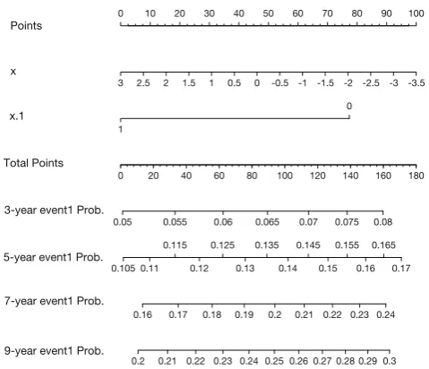
> surv <- Survival(mod) > nom.sur<- nomogram(mod, fun=list(function(x) 1-surv(3,x), function(x) 1-surv(5,x),
function(x) 1-surv(7,x), function(x) 1-surv(9,x)),
funlabel=c("3-year event1 Prob.", "5-year event1 Prob.",
"7-year event1 Prob.", "9-year event1 Prob."), lp=F)
> plot(nom.sur, fun.side=list(rep(1,8), c(1,1,1,3,1,3,1,3,1,3,1,3,1,3,1), rep(1,10),rep(1,12)))
cumulative incidence will be calculated. The function 1-surv() is to create the cause-specific cumulative incidence. The fun.side argument specifies the side on which the tick marks are positioned, with 1 indicating below the axis and 3 above the axis (Figure 1). This argument aims to avoid potential overlap between axis labels.
Comparison with the result from crr() function
To make sure that the result obtained from the subdistribution hazards model as described above is in consistent with the result from the crr() function, we make a comparison in this section. The parameter estimates of the two methods are the same except for differences that are explained by the stopping criterion in the likelihood maximization. However, the estimates of the standard errors are slightly different. The coefficients of the subdistribution hazard model can be obtained as follows:
> mod$coef
x x.1
-0.04711762 -0.23700849
Regression modeling of the subdistribution function can be performed using the crr() function as well (3):
> library(cmprsk)
> mod.crr<-crr(df$time,df$cause, cov1=df[,c("x","x.1")],
failcode=1, cencode=0)
The regression coefficient obtained from the crr() function can be examined by the following way:
> mod.crr
The coefficients obtained from crr() function match well to that obtained from cph() function.
Conclusions
This tutorial provides a step-by-step approach to the generation of a nomogram for survival data in the presence of a competing event. The tutorial only considered right censored data, but the same approach can be used for left truncated data. While the function crr() contained in the cmprsk package can be used for subdistribution hazard modeling, which has the one-to-one correspondence to the cumulative incidence, it cannot be directly passed to the nomogram() function for drawing a nomogram. Alternatively, the subdistribution can be estimated by a product-limit estimator, which is shown to be equivalent to that estimated by the Aalen-Johansen method. The proportional subdistribution hazards model is not a product-limit structure. However, the same idea of weights is used, because the subdistribution is estimated. This can be realized by setting weights for subjects experiencing competing events in crprep() function. Then the result
1PJOUT
can be passed to cph() function in the rms package. The object returned by the cph() function can be passed to the nomogram() function to draw a nomogram.
Acknowledgements
Funding: The study was funded by Zhejiang Engineering
Research Center of Intelligent Medicine (2016E10011) from the First Affiliated Hospital of Wenzhou Medical University.
Footnote
Conflicts of Interest: The authors have no conflicts of interest
to declare.
References
1. Robins JM, Finkelstein DM. Correcting for
noncompliance and dependent censoring in an AIDS Clinical Trial with inverse probability of censoring weighted (IPCW) log-rank tests. Biometrics 2000;56:779-88.
2. Fine JP, Gray RJ. A proportional hazards model for the subdistribution of a competing risk. J Am Stat Assoc 1999;94:496-509.
3. Zhang Z. Survival analysis in the presence of competing
risks. Ann Transl Med 2017;5:47.
4. Kattan MW, Heller G, Brennan MF. A competing-risks nomogram for sarcoma-specific death following local recurrence. Stat Med 2003;22:3515-25.
5. de Wreede LC, Fiocco M, Putter H. mstate: an R package for the analysis of competing risks and multi-state models. J Stat Softw 2011;38:1-30.
6. Beyersmann J, Latouche A, Buchholz A, et al. Simulating competing risks data in survival analysis. Stat Med 2009;28:956-71.
7. Moriña D, Navarro A. Competing risks simulation with the survsim R package. Commun Stat Simul Comput 2016;8:1-11.
8. Geskus RB. Cause-specific cumulative incidence estimation and the fine and gray model under both left truncation and right censoring. Biometrics 2011;67:39-49.
9. Geskus RB. Data analysis with competing risks and intermediate states. CRC Press, 2016.
10. Donoghoe MW, Gebski V. The importance of censoring in competing risks analysis of the subdistribution hazard. BMC Med Res Methodol 2017;17:52.
11. Zhang Z, Kattan MW. Drawing Nomograms with R: applications to categorical outcome and survival data. Ann Transl Med 2017;5:211.
12. Harrell FE. Regression Modeling Strategies. New York, NY: Springer New York, 2001.