Computer-Aided Security Surveillance
DESIGN OF THE
Q
UO
V
ADIS OBJECT TRACKER
Vincent van der Tuin
Master’s thesis November 2007
Human Media Interaction Group Faculty of Electrical Engineering, Mathematics and Computer Science
Abstract
Table of Contents
Abstract...2
Table of Contents...3
Chapter 1: Introduction...4
Chapter 2: Literature survey ...5
2.1. Introduction ...5
2.2. Calibration ...5
2.3. Background separation ...6
2.4. Tracking...6
2.4.1. Introduction ...6
2.4.2. A taxonomy of tracking tasks ...7
2.4.3. Short and medium term tracking ...7
2.4.4. Tracking with multiple cameras ...8
2.4.5. Long-term tracking ...8
2.5. Summary...8
Chapter 3: Approach overview...10
Chapter 4: Background separation ...11
4.1. Introduction ...11
4.2. Approach ...11
4.2.1. Static differencing...11
4.2.2. Temporal differencing ...12
4.2.3. Combining the approaches ...12
4.3. Implementation...12
4.3.1. Pipeline ...12
4.3.2. Processors ...13
Chapter 5: Blob tracking...18
5.1. Introduction ...18
5.2. The basics ...18
5.3. Overlap tracker ...19
5.4. Histogram tracker ...20
5.5. Cascaded tracker...21
5.6. Left luggage alerter...21
5.7. Comparison with other tracking methods...21
Chapter 6: Homographic transform ...23
Chapter 7: Results and evaluation ...25
7.1. Blob tracker evaluation...25
7.2. Homographic transform evaluation ...30
Chapter 8: Conclusions and future work ...34
Legal note on the datasets...34
References ...35
Chapter 1: Introduction
In recent years, due to an increased awareness of terrorism and related risks, and the advent of cheaper cameras and more powerful image processing techniques, the use of cameras for sur-veillance has increased. However, installing cameras is no goal in itself, and there is very little use for the camera footage if no sort of threat analysis is performed on it. An example of such a threat analysis is the so-called left luggage detection, i.e. detecting objects that have been dropped off at the scene being abandoned by the person who brought them there.
Performing this monitoring manually can require amounts of manpower up to infeasible lev-els, and the concentration of a human observer can lapse. This is where computer vision comes in as an automated aid to such an observer.
We examine the issues involved in designing computer vision software systems for security surveillance and present an approach to tracking multiple persons and objects in an indoor environment.
We present the design of a system that can track several people or objects simultaneously in an indoor environment, and retain the object’s identity labelling after occlusion. It will flag immobile objects as potential threats.
The first component of the system is the background separator, which separates the objects to track from the rest of the footage. It uses a combination of a motion detector and a back-ground subtractor which needs to be initialised by an auxiliary component that extracts a background image from the footage.
The tracking algorithm is based on a combination of checking for overlapping motion/object regions, paying attention to regions that split and merge to deal with noise and occlusion, and a comparison of object representations by means of colour frequency histograms to help in cases where the overlap tracker would be unable to maintain object identity.
The locations of the detected objects are converted to 2D world coordinates, to facilitate dis-playing and merging detection data streams from multiple cameras. This component needs to be calibrated by input of the world coordinates of four ground plane locations in the camera image.
The data corpus of the PETS 2006 workshop will be used to experimentally evaluate the tracking algorithm, the threat alerter and the coordinate conversion.
Chapter 2: Literature survey
2.1. Introduction
In this chapter, we will investigate the issues surrounding the design of computer vision soft-ware systems for people and object tracking. Prototype systems designed in similar projects can track moving objects such as people as they move through the camera footage. We take a look at combining the data received from a network of cameras and assigning a unique and persistent identity to the persons detected, so they can be tracked throughout the network. Note that this overview will mainly be concerned with tracking persons as a whole, rather than with pose estimation or motion analysis [Pop06], although some techniques will require some subdivision, e.g. face recognition.
This chapter aims to give an idea of the technical challenges involved in the design of such a system, and the existing research into how to solve them. Although this overview is unlikely to be exhaustive, it will still give a representative impression of problems and solutions in-volved.
2.2. Calibration
Camera calibration is the determination of the parameters that govern the relation between the 2D image coordinates and the 3D world coordinate system. This is required if the system is supposed to determine the full 3D or projected 2D world coordinates of detected objects, e.g. for displaying on a map. For simpler applications, such as object detection or recognition, this may not always be necessary. Alternatively, particular relations, such as the locations of the edges of the field of view (FOV) of a particular camera in the image of another camera can be learned automatically [Kha01, Kha03].
Camera calibration values can be divided into intrinsic and extrinsic properties, also known as internal and external. Intrinsic properties are specific to and generally invariant for a particu-lar camera. These include values such as the focal length of the lens, scaling and possibly dis-tortion factors. Extrinsic properties, on the other hand, refer to the camera in its environment, i.e. to the location and orientation of the camera and thus also to the relative positions of cam-eras in a multi-camera network. Note that instead of determining both groups of parameters explicitly, they can also be represented by coordinate transformations from the camera image to a common world coordinate system [Bak00, Wil03].
Calibration can be performed manually, but this is labour intensive, making it infeasible if the network is large and/or dynamic. Therefore, several automatic or semi-automatic camera cali-bration methods have been developed. Most of these methods assume at least some overlap-ping of the fields of view to determine the relative extrinsic properties of the cameras. If there is no such overlapping, it is still possible to estimate the network topology, e.g. in terms of probable adjacency [Jav03].
2.3. Background separation
The vision system needs to know what parts of the image contain objects of interest that should be tracked, and what parts just contains walls, floors and other objects, usually static, that should be ignored for the purposes of tracking. This process is called background tion. It is related, but not identical to motion detection, as although most background separa-tion algorithms are based on mosepara-tion detecsepara-tion, if a system is supposed to track a particular object, it should keep doing so if the object stops moving. However, it would also be possible to deal with this problem in higher-level reasoning stages.
The simplest way to construct a motion detection algorithm is to compute the pixel-wise dif-ference between two consecutive frames and threshold the result [Tui05, Lip98]. This usually generates only an outline of the moving object, rather than all the pixels of the object. It also introduces a systematic inaccuracy by including a trail of pixels at which the object was in the previous frame, but currently isn’t anymore. It is possible to include corrective measures to compensate for this trail and to include additional measures like template matching in case the object motion halts [Lip98].
A basic form of a common method for background separation which does not suffer from this is to obtain a reference background image and to compute and threshold the difference with that [Spa05]. This method, however, cannot compensate for changes in illumination of the scene, either abruptly by someone opening a door or flipping a light switch, or by gradual changes such as those caused by daylight. One way to adaptively compute the background image is to take the median over time [Sie03]. Another common way is to model each pixel using one or more Gaussian distributions [Ell02, McK00, Rie03, Wre97, Zha01].
Foreground images generated like this will probably still contain noise and other unwanted areas, such as the ones caused by shadows. These shadows could be rejected by checking whether the change in chromaticity is negligible [McK00, Ell02, Tho05]. Also, there will probably be gaps in the detected areas, which could be corrected by post-processing the re-sults with morphological operations such as closing [Rie03, McK00, Zha01], although this probably isn’t worth the computational effort if only a bounding box of the object is required. It will, however, alleviate the problem of a single person being detected as several blobs, for which corrective measures such as blob clustering would have to be used [Kru00].
It is also possible to combine these algorithms with other modalities than colour spaces. For instance, when using multiple cameras pointed at the same area, one could use the results of stereo range finding [Dar00, Har98, Kru00].
All methods described so far have assumed that the camera remains stationary. If this is not the case, additional compensation is to be performed, e.g. by matching features such as edges [Cai95].
2.4. Tracking
2.4.1. Introduction
2.4.2. A taxonomy of tracking tasks
Tracking systems meant for different purposes have different requirements and characteris-tics. To structure our discussion, we will first create a classification of tracking system types according to what they’re required to do, and in what environment.
The first distinction we need to make here is that of track lifetime, i.e. for how long the sys-tem assigns the same identity to the object it follows, as the technical requirements for meth-ods to perform this differ. Also, it needs to be taken into account whether the assumption is made that only one person to be tracked is present in the image at any given time, or that there can be multiple simultaneously.
The various kinds of track lengths we will consider are as follows:
• Short-term or continuous path tracking, where a tracked person can be absent from the de-tection for at most a few frames.
• Medium-term tracking, where a person re-enters the tracked area after minutes or hours. • Long-term tracking, where the person re-enters the area after days or longer. Basically, this
is identification, i.e. linking the detected person to his or her real-world identity, followed by a shorter-term track.
A final distinction to be made is whether the object is being tracked by a single camera or whether it is within the field of view of multiple cameras.
Now that we have defined the taxonomy of tasks and requirements involved in tracking, we will investigate the various methods of performing this. Note that some methods are not strictly confined to a single class as described above. For instance, methods for obtaining an object’s identity for any track length can achieve a similar goal to that of a system that tries to re-label short-term object identities after occlusion by extrapolating their paths.
2.4.3. Short and medium term tracking
For short-term tracking, a number of relatively simple methods can be employed. If there is no occlusion, a simple check for overlapping bounding boxes can maintain short-term iden-tity. Faced with occlusion, one way to maintain short-term identity is probabilistically track-ing and examintrack-ing the object’s path, headtrack-ing and velocity. Methods such as Kalman filters [Ass94, Cai95, Ell02, Jav03, Rie03, Sie03] or particle filters [Tui05, Tan04, Tho05] can be used here. As mentioned before, this can also be handled by longer-term tracking methods which aim to recognise the object by its features rather than its expected location.
For short-term tracking of people, we need to have some feature or features to match. One such feature is the height or aspect ratio of the bounding box [Cai98, Ell02] or the real-world height of the person being tracked, which can be computed even in a monocular system by including a priori knowledge of the environment of it in the form of a model of the environ-ment’s geometry and/or a ground plane assumption [Agg98, Rie03, Spa05]. Usefulness of height as an auxiliary feature for long-term tracking has also been reported [Dar00].
Generic template matching approaches are often not very well applicable to people tracking due to the non-rigidity of the human body. Another popular short-term tracking method is to make use of colour or intensity features. Specific points on a person could be picked for this [Cai94, Cai98], or the whole person could be used to compute a mean colour probability [Kru00, McK00, Por03, Ell02]. Alternatively, the person could be subdivided into several blobs with separate representations, either segmented by connected components analysis [Kru00, McK00, Por03] or representing specific parts of the person such as the face, hair, skin or clothes [Dar00, Reh97]. Instead of using just the colour, one could also opt to analyse the texture [Nug94].
2.4.4. Tracking with multiple cameras
For multiple cameras observing the same person, the problem is slightly different. A draw-back of using the colour approaches for multi-camera systems is that cameras are usually not consistent in how they perceive colours. This can be compensated for by using additional calibration to normalise between the cameras [Por03]. One could also choose not to use ap-pearance features, but to combine location tracking results from multiple cameras by using the results of external camera calibration to compute a coordinate homography, which will map the coordinates reported by various cameras onto a global coordinate system [Dev04, Ell02, Lee00, Sat94, Uts98].
2.4.5. Long-term tracking
For long-term tracking of people, approaches based on things like clothing colour can obvi-ously be ruled out. Other biometric features can however be found in the image and used in conjunction, such as the height and the face [Dar00]. Gait recognition could be employed if the view of the person is large enough for reliable segmentation [Lee02].
2.5. Summary
Designers of software systems for computer-aided surveillance and tracking need to create a number of system components posing technical challenges. We have discussed a number of these main components, problems involved in their implementation and possible ways of solving them.
If we want to be able to map the image coordinates of objects observed to real-world coordi-nates (2D or 3D) for display or comparison purposes, the cameras used need to be calibrated. Camera calibration parameters are often divided into intrinsic parameters, which are specific to the camera itself, and extrinsic parameters, which refer to the camera’s positioning in its environment. Some methods, however, do not employ this distinction, but represent them in another way, e.g. directly as a coordinate transformation function.
The required camera calibration parameters can be measured and computed manually, but automated techniques have also been developed for calibration, making this less labour inten-sive and therefore more scalable. Many of these methods use a priori knowledge of certain objects in the scene, such as a calibration grid, or use object motion. This can also be used to determine relative positioning of cameras in case the system uses several cameras with over-lapping FOVs simultaneously.
Not all areas selected using these frame comparison-based methods may actually be objects of interest; they could be caused by effects such as shadows or sensor noise. Additional steps can be taken to eliminate these from the detection, e.g. checking for negligible chromaticity change to remove shadows. Post-processing with morphological operations such as closing can fix gaps in detected objects.
To keep track of objects of interest once they have been found, we require a tracking algo-rithm. Technical requirements for tracking algorithms differ largely depending on the sys-tem’s goal and environment. Some important points to consider are for how long the system should be able to track its target, whether there is just one target to track at any given time or whether there can be multiple (possible occluding), and whether the system processes the feed from just one camera or whether it should merge the data from several cameras.
A simple method for tracking targets on a continuous path is checking for overlap of their out-lines or bounding boxes. This method cannot deal with occlusion. Methods that can augment or replace it to be able to track through occlusion are e.g. predicting the object’s path and ve-locity with methods such as Kalman filters, or matching the object’s appearance, for instance by building and comparing a colour histogram of the target.
To reinitialise tracking of people by identifying them after a longer time, it is possible to use biometric approaches such as face or gait recognition.
Chapter 3: Approach overview
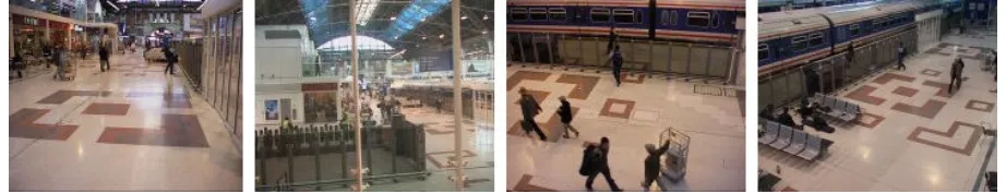
After the broad overview of issues and methods in the previous chapter, we have to set bounds for the domain of the system we are presenting, and select methods that are suited to our situation. Our approach was designed to be applied to an indoor real world public envi-ronment. It will be tested on the data corpus of the PETS 2006 workshop [PET06], containing footage of such an environment (a train station), recorded with a number of static cameras pointed at the same area from several directions. Several people move through this area, in-cluding a test subject who leaves his backpack. Our system should be able to track them si-multaneously. The relative real-world coordinates of several points on the visible part of the station floor are specified for calibration purposes.
Figure 3.1: Sample images from the PETS 2006 cameras
In order for our system to achieve its vision task, the camera footage is processed by several subsequent components, forming a processing pipeline (Figure 3.2).
Figure 3.2: System pipeline overview
The system first separates objects that are of interest to the system for tracking purposes (the foreground) from the rest of the image, depicting the scene’s background. This is done by a combination of static background subtraction [Lip98] and temporal differencing, to detect both moving and static objects of interest. To create the static background, a static camera is assumed, but the availability of a frame containing no foreground objects is not required, as it can be estimated from a series of frames containing moving foreground objects, using a tem-poral median filter [Sie03].
Once we know which pixels of the frame are to be tracked, they are grouped into connected components (blobs) and handed to the blob tracking component. This component’s task is to match blobs observed in different frames as having the same identity, i.e. they’re depictions of the same object or person, so we can track them through time. Our approach combines blob identity maintenance by checking for overlapping blobs [Auv06] and keeping track of blob interaction states such as merging and splitting [Ell02] with matching blob representations in the form of colour frequency histograms [Kru00] to obtain an efficient algorithm that is able to maintain tracked blob identity beyond these blob interactions caused by noise and occlu-sion.
Blob positions are then converted to world coordinates. This means that output on positions of objects of interest can be displayed in a floor plan style, and alert trigger conditions can be expressed in real-world distances. It also facilitates merging the data with that of other cam-eras during future projects. A homographic transformation [Cri99] is used to perform this conversion, which is easier to calibrate than full camera calibration [Tsa86], while still giving satisfactory and useful results. The system thus requires less calibration points, i.e. at least four corresponding pairs of 2D image/world coordinates to estimate the transformation.
Background estimator Calibration
Chapter 4: Background separation
4.1. Introduction
The background separation step is the part of the vision processing pipeline in which the sys-tem decides whether any part of the image is an object that may be of interest to the syssys-tem and should be tracked, or that it is part of the background. First, a number of approaches and their pros and cons will be discussed. A description follows of how this is actually achieved in the prototype implementation, focussing first on the system as a whole and then on its indi-vidual vision processing filters.
4.2. Approach
Because there are several approaches to background separation, and which is best depends largely on the situation that is to be processed, a number of methods have been implemented.
4.2.1. Static differencing
This method works by computing the difference between the incoming (colour) image and an image of the background without any foreground objects, for each colour channel separately. If no such image is available, one can be constructed by computing the median per pixel and channel over a number of images spread throughout a dataset of images that also contain foreground objects (persons etc.) [Sie03]. Assuming the scene is not too crowded, any par-ticular place will be unoccupied for most of the time, i.e. it will show the background. There-fore, a median of any given pixel will give us the background colour, even though the absence of foreground objects does not have to occur throughout the whole scene simultaneously; a normal bit of surveillance footage can be used, as long as people that should be classified as foreground are moving and there are not so many people that some parts of the background will be occluded most of the time. If this is not the case, footage containing less heavy traffic will need to be selected in order for this method to work.
Selecting the foreground pixels can now be done by applying a minimum threshold to the ab-solute difference [Sie03, Spa05]. This threshold can be implemented at different levels of granularity: globally, per colour channel, or even per image section or pixel. The finer the granularity, the finer the algorithm can be tuned, but this is likely to increase the amount of data required to train or tune the system.
Differences can not only be caused by foreground objects showing up, but also by the shad-ows they cast. This will not usually be the kind of things that we wish to track, though, so we seek a way to remove these shadows from our detection. A way to do this is by taking into account that shadows are a darker variety of the original background colour at that specific location [Ell02, Tho05]. Therefore, we convert the image to the Hue-Saturation-Value colour space [For03] before thresholding, so we can classify pixels with negligible hue difference as background (shadow).
Detected foreground objects that are so small that they are likely to be just noise can be re-moved during a post-processing step. Likewise, objects that are only a few pixels apart may have been split due to noise. This will be covered in greater detail in the implementation sec-tion.
e.g. a change in lighting conditions. How to automatically adapt the background without loss of the ability to detect static foreground objects is not clear-cut.
4.2.2. Temporal differencing
Instead of computing a static background from a dataset, two images that are one or a few frames apart in the video sequence can be compared in the same way as with static differenc-ing. Sections that contain a moving object in one of the frames will cause an outline of the object to appear in the resulting difference image, as demonstrated in the image below [Cai95, Tui05, Lip98].
The difference of the images will now automatically and quickly adapt to changes in the background, such as the ones caused by lighting change. Foreground objects that are perfectly still, however, such as left luggage, cannot be detected by this method without additional measures. Also, the half of the outline that is ‘trailing’ the moving object shows up because in the current frame the object isn’t at that location anymore; this could cause a systematic inac-curacy in a naïve implementation of a method to measure the object’s location (e.g. comput-ing the outline’s centroid).
Figure 4.1: Temporal differencing
4.2.3. Combining the approaches
There are a couple of ways how these methods can be combined to create a “best of breeds” system. One of the most straightforward ways is to apply a logical disjunction (‘or’) to the foreground masks generated by both approaches, but this does not optimally harness the bene-fits of both approaches. Another option is to construct a system that tries to estimate which method will work best at a certain moment and switches to it, by classifying the situation or assigning a confidence measure to the foreground masks. For example, a system that uses static differencing by default could detect the flipping of a light switch as a steep increase in foreground pixels, and temporarily switch to temporal differencing while the static back-ground is updated.
4.3. Implementation
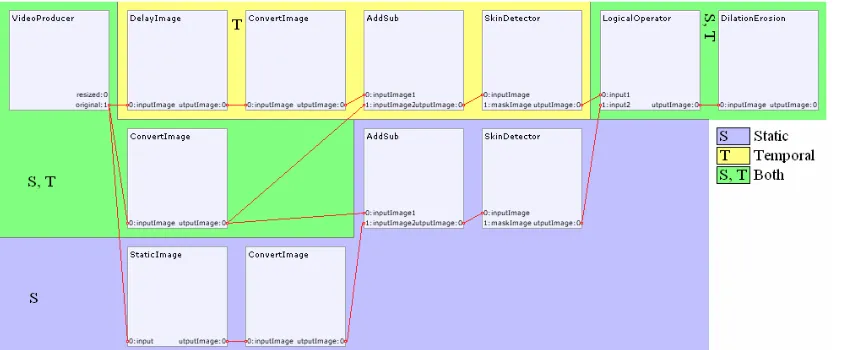
An implementation of a combined static/temporal differencing system as described above has been made based on the HMI group’s ParleVision framework, in which several vision filters, known as processors, are chained together to form a vision processing pipeline [Bra04]. This allows for a very modular approach.
We will first discuss the pipeline, which determines the data flow and the behaviour of the system as a whole, and then take a closer look at the processors which it is made of.
4.3.1. Pipeline
Figure 4.2: Background separation pipeline
4.3.1.1. Static differencing pipeline
The input video frames are delivered by a special class of ParleVision processor called a pro-ducer; in this case a VideoProducer is used, which reads the frames from a video file. The static background image used here for differencing is computed by an external tool using the median method described in Section 4.2.1 and loaded into the pipeline by the StaticImage processor. Both the input frame and the static background frame are converted to the HSV colour space before their pixel-wise absolute difference is computed, as computing the differ-ence in this colour space will help with shadow removal, as described in the Approach sec-tion. These differences are thresholded to obtain a binary image labelling the foreground and background pixels. Detected foreground blobs (areas of connected foreground pixels) that are so small that they are likely to be caused by noise are removed by morphological erosion (and subsequent dilation to reduce changes to other foreground blobs) [Bre00] and enforcing a minimum amount of pixels per blob. See the Processors section for examples.
4.3.1.2. Temporal differencing pipeline
The temporal differencing pipeline works in much the same way as the static differencing pipeline, but now the static image loader is replaced by a processor that outputs a frame that is a few frames older than the current frame, so that the outlines of moving objects should now show up in the difference image.
4.3.1.3. Final combining pipeline
As both algorithms now output a binary image, we can apply a simple logical disjunction (‘or’) to obtain a combined result. A dilation and erosion step are applied to prevent fore-ground objects being split into several blobs by the effects of noise.
4.3.2. Processors
4.3.2.1. VideoProducer
Inputs: None
Outputs: resized, original
The VideoProducer reads input frames from a video file (in AVI, WMV or MPEG format) and delivers them to the pipe-line for processing. The frames are also offered at a normalised size (320×240 pixels). An option has been added to ignore the frame rate specified in the video file and output the frames as fast as they can be processed by the host system.
4.3.2.2. CameraProducer
Inputs: None Outputs: source
The CameraProducer obtains input frames from a Microsoft DirectShow-compatible device such as a webcam and delivers them to the pipeline for processing.
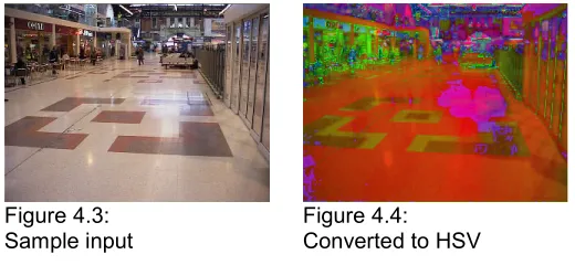
4.3.2.3. ConvertImage
Inputs: inputImage Outputs: outputImage
The ConvertImage processor converts the incoming colour (RGB) image to a specified other colour space: grey scale, Hue-Saturation-Value (HSV) or YCrCb.
Figure 4.3: Figure 4.4: Sample input Converted to HSV
4.3.2.4. AddSub
Inputs: inputImage1, inputImage2 Outputs: outputImage
The AddSub processor computes the pixel-wise sum or differ-ence of two input images, for every colour channel separately. In addition to the normal difference, the absolute difference can be chosen as output. Of this latter operation, an implemen-tation has been added which makes fewer internal image buffer copies, to improve efficiency.
Figure 4.5: Figure 4.6: Figure 4.7:
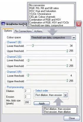
4.3.2.5. SkinDetector
Inputs: inputImage, maskImage Outputs: outputImage
The SkinDetector processor finds regions of interest (ROIs) by means of colour space conversions (or colour channel ratio computations) and applying configurable thresholding rules to the pixels to obtain a binary (black-and-white) image indicat-ing the ROIs. In the early versions of this processor, the col-ours to be identified were skin tones, hence the name, although its applicability is more generic. A built-in colour space con-version can be selected, or the raw input can be thresholded to process an RGB colour image or one pre-processed by a proc-essor such as ConvertImage. Lower and upper thresholds can be set for up to three separate colour channels.
The binary ROI map can be post-processed by applying a specified number of iterations of a morphological erosion and/or dilation operator (see the next processor). Additionally,
connected components (blobs) can be automatically removed if the number of pixels they consist of falls below a certain threshold.
The example below shows the result of thresholding an input image obtained by converting two images to the HSV colour space and computing the absolute difference. No post-processing has been applied.
Figure 4.8: Figure 4.9:
Input image Output image
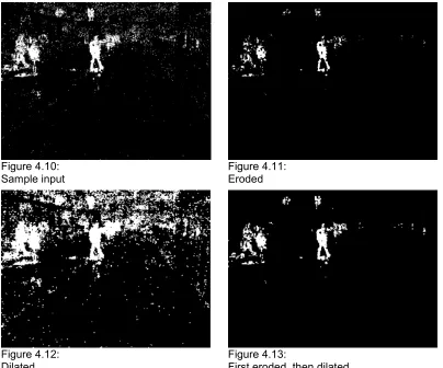
4.3.2.6. DilationErosion
Inputs: inputImage Outputs: outputImage
Figure 4.10: Figure 4.11:
Sample input Eroded
Figure 4.12: Figure 4.13:
Dilated First eroded, then dilated
4.3.2.7. StaticImage
Inputs: input Outputs: outputImage
The StaticImage processor delivers the same image for every frame. Unlike the ImageProducer processor, it has an input so it can deliver these images in sync with the rest of the pipeline, thus avoiding the recomputation issues associated with Parle-Vision pipelines with multiple producers.
The image to output can either be read from an image file or
grabbed from the input pin. Using this latter function, it can also be used to keep a particular frame in memory anywhere in the pipeline, for further processing.
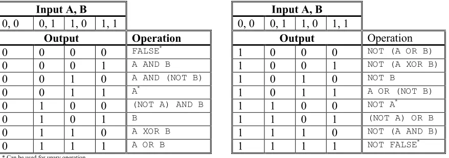
4.3.2.8. LogicalOperator
Inputs: input1, input2 Outputs: outputImage
The LogicalOperator processor applies a unary or binary logi-cal operator to binary (black-and-white) images, such as the ROI map produced by the SkinDetector processor. The set of available operators has been chosen in such a way that, in
Input A, B Input A, B
0, 0 0, 1 1, 0 1, 1 0, 0 0, 1 1, 0 1, 1
Output Operation Output Operation
0 0 0 0 FALSE* 1 0 0 0 NOT (A OR B)
0 0 0 1 A AND B 1 0 0 1 NOT (A XOR B)
0 0 1 0 A AND (NOT B) 1 0 1 0 NOT B
0 0 1 1 A* 1 0 1 1 A OR (NOT B)
0 1 0 0 (NOT A) AND B 1 1 0 0 NOT A*
0 1 0 1 B 1 1 0 1 (NOT A) OR B
0 1 1 0 A XOR B 1 1 1 0 NOT (A AND B)
0 1 1 1 A OR B 1 1 1 1 NOT FALSE*
* Can be used for unary operation
Table 4.1: LogicalOperator truth table
A few example operations:
Figure 4.14: LogicalOperator examples
4.3.2.9. DelayImage
Inputs: inputImage Outputs: outputImage
Chapter 5: Blob tracking
5.1. Introduction
Now that we’ve obtained the foreground pixels from the background segmentation part of the system pipeline, they will be grouped into blobs of 4-connected pixels on a frame-by-frame basis. These blobs will form the basis for our tracking implementation. Now, we wish to pair up blobs from different frames as having the same identity, i.e. they’re depictions of the same object or person, so we can track them through time.
There are a couple of complications when it comes to just tracking blobs to tracking objects on a higher semantic level, as blobs do not always have a one-to-one correspondence to the objects they represent. As we’ve defined our unit to track as a connected component of pixels, these may merge, split or be temporarily lost due to factors such as sensor noise or occlusion. An approach to this tracking task will be presented in this chapter.
5.2. The basics
We want to achieve the assigning of a persistent identity (represented by an ID number we’ll refer to as the path ID) to objects being tracked (e.g. persons). At an implementation level, however, these IDs are assigned to blobs. Ideally, a path ID refers to an object rather than just a blob. We’ll try to keep this matching by analysing blob interactions such as merging and splitting.
Basically, to perform the assigning of this path ID over multiple frames, we attempt to match all blobs in the current frame to the blobs in the previous frame that should be assigned the same identity, taking into account the fact that blobs may split and merge due to the reasons mentioned in the previous section. Therefore, for each input frame, in addition to the determi-nation of its path ID, each blob gets a state that indicates whether one of these blob interac-tions has taken place. The following list shows the states that can be assigned to a blob during an iteration of the algorithm, during which the blobs of one frame are processed [Ell02]. The Prev and Curr columns list how many blobs in the previous and current frame take part in that type of blob interaction.
State Description Prev. Curr.
Matched Matched to a previously found blob 1 1
Split Broken off of a previously found blob 1 2..n Merged Two or more previously found blobs have merged 2..n 1
New Blob could not be matched to a previously found blob 0 1
Unknown Temporary state to indicate that a blob hasn’t been processed yet
N/A 1
Table 5.1: Tracked blob states
A Missing (1/0) state for previously found blobs that disappear from the footage has not been included as iterating over the blobs of the current frame to determine their state would not lead to such an assignment.
This creates a combined algorithm with a ‘cascading’ structure, i.e. blobs that cannot reliably be handled by a particular algorithm will be handed on to the next. Both constituent parts and the combination will be examined in more detail in the following sections.
5.3. Overlap tracker
The overlap tracker is based on the assumption that if we overlay the current image of a mov-ing blob with its image in the previous frame, these images will partially overlap. This as-sumption holds if the object’s velocity is not too high in relation to its size and the frame rate. If it is, predictive methods such as Kalman filters may help. We’ll revisit that point in the Comparison section.
To compensate for the fact that blobs do not always overlap one-on-one, the detection of split and merged blobs is integrated into this algorithm.
Consider the following overlaid current and previous frames:
Figure 5.1: Overlap tracker cases
The blobs in this example move predominantly to the right. A number of possible scenarios have been displayed. We consider a pair of blobs to be overlapping if the number of pixels they have in common exceeds a preset proportion of the area of the constituent blob (merged or split). A blob in the current frame (‘new’) overlapping with exactly one blob in the previ-ous frame (‘old’) will receive the old blob’s path ID and the Matched state. If an old blob overlaps with two or more new blobs, they get the Split state. As the old blob may have been the result of a prior merge, the histogram tracker may have a record of these blobs, and they will be handed to this tracker to determine the path IDs. If two or more old blobs overlap with one new blob, it is Merged, and is assigned the path ID of the largest old blob, as the other blobs are assumed to be either blobs that were incorrectly segmented as a separate blob due to noise, or moving objects that are causing dynamic occlusion, for which overlap tracking of the separate objects will effectively be suspended for the duration of the occlusion. Any re-maining new blobs that are not categorised as Matched, Split or Merged will continue on to the histogram tracker, which will determine whether the blob can be Matched to a previously observed blob, or that it will get the New state and its data will be associated with a new path ID.
5.4. Histogram tracker
Any blobs in the current frame that could not be assigned a path ID by the overlap tracker, either because they’re the result of a split or because no blob could be found in the previous frame to match it with, will end up at the histogram tracker to get their path ID determined. As briefly mentioned previously, the histogram tracker uses colour features rather than spatial features to match blobs. This allows the histogram tracker to reassociate a blob with its proper path ID after occlusion or overlap tracker glitches.
To achieve this, the image of the blob in the Hue-Saturation-Value colour space is converted into a colour frequency histogram, with each axis of the colour space quantised into a number of bins that is high enough to distinguish the blobs, but low enough to give rise to similar his-tograms for multiple observations of the same object. In our implementation, the channels are quantised into 10 bins each. The histogram is normalised with respect to the sum of the bins, so that the influence of the size of the blob is reduced. This normalisation is performed as fol-lows:
Ha,b = bin b of histogram a
S = target sum (preset normalisation constant)
Scale (multiply) every bin of Ha by the same value so that ∑(Ha,b) = S
The tracker keeps a list of observed blobs with their most recent histograms, containing one entry for each path ID. This list is called the blob inventory. It is updated whenever a match to a path ID is made, even if this is by the overlap tracker. This update means simply writing all computed metadata of the current frame’s blob to the inventory entry, although e.g. a more gradual update of the colour histogram could be devised.
For every blob that is handed to it by the overlap tracker for matching, the histogram tracker iterates through this blob inventory and computes a similarity measure between the blob to match and the blob in the inventory. This similarity measure is computed as the cumulative absolute difference between the bins of two histograms, and finding the best match is there-fore a matter of minimising this difference. If the best match meets a preset matching thresh-old, the blob to match is assigned the path ID of this inventory blob. If no inventory blob meets the threshold, a new path ID is assigned to the blob and it is added to the inventory as a new blob.
If objects need to be tracked that are coloured very similarly, making ID assignments in the order in which blobs are encountered may not suffice, which could be solved by using an al-gorithm that minimises the total difference between all pairs of blobs to match and inventory blobs.
Figure 5.2: Figure 5.3: Figure 5.4:
Sample input frame HSV image of tracked blobs Histogram graphs with their path IDs. U indicates
a matched (updated) blob.
S
at
.
Hue
5.5. Cascaded tracker
Now that we’ve seen the constituent tracking algorithms, let’s recap and take a look at how every blob in the current frame is processed by the cascaded tracker. The following flowchart shows the basic process of determining a blob’s state and path ID. Note, however, that an ef-ficient implementation will compute the metadata of all new blobs first, as described in Sec-tion 5.3.
Figure 5.5: Blob tracker flowchart
5.6. Left luggage alerter
As an example of an automated threat analysis that can be performed using the tracking data, we created a simple left luggage alerter that should find left luggage objects and mark them in the system’s UI. We do this by detecting blobs that remain stationary. People and luggage are distinguished by imposing a maximum height for luggage items (50 pixels). A blob is considered stationary if the minimum and maximum of its last 30 centroids (just over a second) are no more than 10 pixels apart on ei-ther the X or Y axis.
5.7. Comparison with other tracking methods
The use of colour histograms can be compared to mean-shift algorithms such as the Continu-ously Adaptive Mean Shift (CAMSHIFT) algorithm [Bra98], in which the colour histogram of the colour or object sought is treated as a probability distribution to determine whether frame pixels are likely to belong to the object. The algorithm then applies iterations of a gra-dient ascent approach to shift the tracked object to its most likely position in the frame.
CAMSHIFT thus combines the use of spatial and colour features into a single operation, whereas in our approach these are treated separately. This allows us to use just the spatial fea-tures for a computationally efficient continuous-path tracking algorithm (the overlap tracker), as it operates on binary images and requires no iterations. Also, it allows us to use the colour
Segment new blob, compute metadata (contour, histogram etc.) ID of largest old blob
features to reinitialise tracking multiple objects after they occlude each other. The version of CAMSHIFT described would be unable to track several objects simultaneously if one is fully occluded, although it might prove useful during partial occlusion.
Our overlap tracker is similar to the tracking approach used by Auvinet et al. [Auv06]. The authors remark that this tracker alone does not suffice to maintain identity after dynamic oc-clusion (blob merge and split), and suggest using colour histograms for the relabelling. Our cascaded tracker is an example of such a combination.
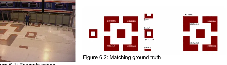
Chapter 6: Homographic transform
As mentioned in Chapter 3, we require a transformation from camera coordinates to world coordinates. Here’s an example transformation task using data from the PETS 2006 workshop [PET06].
Such a conversion can be achieved using a projective transformation, also known as a graphy or homographic transform [Har00]. In general, a 2D homographic transform of homo-geneous coordinates is defined by a 3×3 matrix according to the equation W = H·c, or in more
with W = world coordinates vector and c = camera coordinates vector
One of the nine elements of the transformation matrix H can have a fixed value without loss of generality, as the fact that a homographic transform is equal up to scale means that it has only eight degrees of freedom. This scale factor is represented by S.
Solving for W, we obtain the following expressions for the world coordinates in non-vector form [Wre98]. Note that a division by S has been performed to compensate for the effects of equality up to scale.
Now that we can compute world coordinates from the camera coordinates and the transforma-tion matrix H, we need a way to obtain that matrix. Knowing the 2D coordinates of at least four matching pairs of points in camera and world space gives us the eight equations we need in order to be able to solve this equation for H. If there are exactly four pairs the solution will be exact, if there are more, it will have to be estimated by a minimisation scheme.
We now rewrite the system to an equation of the form A·x = b, with x and b column vectors, so it can be solved with standard least square estimation methods [Cri99]:
Singular Value Decomposition or the Moore-Penrose pseudoinverse:
b
This transformation can be applied iteratively to the pixels of an image to warp it. Pixel inter-polation techniques can be employed to improve the quality of the output image if the pixel mapping is not one-to-one.
To determine the coordinates of a tracked blob in the transformed coordinate system, a blob’s centroid is projected onto the baseline of the bounding box (see Figure 6.4).
Chapter 7: Results and evaluation
7.1. Blob tracker evaluation
We will now evaluate the accuracy of our blob tracker. To do this, we will present the tracker with some selected frame ranges from the PETS data corpus, in which the main actor of the dataset’s scenario appears and crosses the field-of-view. To observe the influence of a number of tracker parameters, we will test the same range with different values for these parameters. The parameters we will test are the number of bins in the colour histograms and the similarity measure threshold for the histogram matcher. Also, we will take a look at the results of using different cameras. An input background image is obtained using the method described in Sec-tion 4.2.1.
We will obtain our measure as follows. We’ll look for runs of consecutive frames containing a blob with the same path ID, which we’ll call a track. We ignore all tracks that are shorter than 25 frames (1 second), as we consider them to be noise which the overlap tracker was de-signed to be able to deal with. This means that we will only notice errors that affect tracks held over a longer period of time, which are the ones we are interested in, as those are the only ones which will ever set off activity monitoring alerts such as left luggage detection. For all tracks that last for at least 25 frames (‘long’ tracks), we will look at the blob interactions (merges, splits and matches) that take place for that track’s path ID during its duration. We will manually tally which of these interactions are incorrect, i.e. it breaks the association of the path ID with a real-world object as mentioned in Chapter 5. By dividing this number of errors by the cumulative length of the tracks, we gain the fraction of incorrect decisions taken by the tracker, as the tracker needs to decide once per frame per blob what path ID it should assign the blob. We will also list a number of other statistics, such as the number of tracks and the number of path IDs assigned.
The results in Table 7.1 are obtained using PETS set S1-T1-C camera 1, frames 1800-1950. We compare our default number of 103 bins for the colour histograms to 503, which is a large enough difference to have a measurable effect, and our histogram similarity threshold of 900 to 500, the sum to which the histograms are normalised. A full list of blob interactions ob-served can be found in Appendix A.
The metrics in Tables 7.1 and 7.2 are to be interpreted as follows:
Total track length: This is the cumulative length of the long tracks, in frames. It will be used to compute the error percentage.
# Errors: As explained above, this is the number of incorrect path ID assignments to a blob in a frame, which should be as low as possible.
% Errors: Dividing the number of errors by the total track length gets us the percentage of path ID assignments that were incorrect, which is our main metric. It should also be as low as possible.
Long tracks: The number of long tracks detected, which ideally should match the number of appearances of a person or object to track, as a person moving through the field-of-view should generate one track. If an assignment error is made, the track may be split, resulting in an extra track.
Path IDs: This is the number of unique path IDs assigned during the test. Like long tracks, this should match the number of objects of interest appearing, but unlike the long track count, reappearances of the same object should result in only one path ID.
We will now describe the people and objects present in our dataset selection, and their inter-actions, i.e. touching and occluding causing the blobs representing them to split and merge. This can be used as ground truth. We manually assign numbers to the people observed, con-sistent across the four cameras. The following people appear in our input data:
P1: The data corpus’s main actor. He puts his backpack down on the floor and lingers for a while before moving away from cameras 1 and 2, into the background.
P2: The backpack which is left behind by P1.
P3, P4: Two women walking into the background together, wearing a beige and black coat, respectively.
P5: A station janitor up on the balcony. Janitors wear yellow safety jackets.
P6: A janitor walking into the background.
P7: A man in a black coat up on the balcony.
P8: A janitor waiting near a store.
P9: A woman in a grey coat coming from the background (from camera 1 and 2’s per-spective).
P10: A man in a black coat entering from the left of camera 2’s field of view (FOV).
P11: A janitor loitering in the corner.
In addition to these people, cameras 1 and 2 also see some people moving far off in the back-ground. They will not be labelled individually, as their small appearance in the image will usually be removed by the background separator’s area threshold, and if they do get detected as foreground (e.g. as a larger blob of several occluding people), they could still be removed from the detection by implementing an X axis threshold after the homographic transform. The following images show these people identifier assignments.
Figure 7.2: People ID assignments as seen from camera 2
Figure 7.3: People ID assignments as seen from camera 4
Figure 7.4: Timeline of objects and interactions for camera 1
Figure 7.5: Timeline of objects and interactions for camera 2
Figure 7.7: Timeline of objects and interactions for camera 4
Analysing these graphs according to the rules we’ve set for long tracks at the start of this chapter, we would expect the following values for the long track metric if tracking were per-fect: Camera’s 1, 3 and 4: 5, Camera 2: 8.
The number of path ID’s should of course not be lower than the number of people listed for that camera, but measuring a somewhat higher value does not need to indicate a problem if this is caused by noisy segmentation which can be dealt with by the overlap tracker.
Performing the evaluation on the data mentioned results in the following values:
Bins 103 103 503 503
Threshold 500 900 500 900
Total track length 691 736 466 596
# Errors 2 10 0 2
% Errors 0.289 1.359 0 0.336
Long tracks 7 10 5 7
Total tracks 90 90 128 89
Path IDs 17 10 128 14
Table 7.1: Evaluation metrics for dataset S1-T1-C1 with varying bins/thresholds
The low number of errors for the 503/500 column is deceptive, as this is caused by the fact that the diversity of histograms created by the higher number of bins causes the histogram matcher to split the tracks up into several short tracks, as can be observed from the low num-ber of long tracks in relation to the high numnum-ber of path IDs and total tracks. Requiring less histogram similarity counteracts this effect, as can be seen in the 503/900 column. Also note that the high number of bins has an adverse impact on the computational performance of the tracker. Of the options shown here, 103/500 therefore appears to be the most appropriate set-ting.
The following results were obtained for all four PETS cameras, using set S1-T1-C frames 1800-2150 (103 bins, threshold 900):
Camera 1 2 3 4
Total track length 1327 1457 643 1028
# Errors 10 3 2 7
% Errors 0.754 0.206 0.311 0.681
Long tracks 18 10 6 16
Total tracks 178 97 31 92
Path IDs 11 10 7 14
Table 7.2: Evaluation metrics for dataset S1-T1-C for all cameras
To evaluate the left luggage alerter, we will compare the alert locations reported by the alerter with those listed in the ground truth data included with the PETS data corpus. The following results refer to the alerts generated for the backpack dropped in PETS dataset S1-T1-C:
Camera Location (m) Error (m) #Alerts G.Truth (0.2215, -0.4420) 0 1 1 (0.0308, -0.4580) 0.1914 30
2 - - 11
3 (0.1867, -0.2327) 0.2121 1 4 (0.1867, -0.3395) 0.1082 94
Table 7.3: Evaluation results for alerter
PETS specifies some additional criteria for left luggage. Firstly, luggage is only considered left if it has been abandoned by the person bringing it, i.e. a predetermined minimum distance between luggage and owner is maintained. This means that alerts generated for other objects than the backpack are false positives when evaluated according to the rules of PETS.
Secondly, PETS requires that the abandonment criterion is met for at least 30 seconds without interruption, which means our system’s alert times cannot be compared directly to PETS re-sults.
The extra alerts in our data are generated for stationary blobs such as the ones representing groups of people in the background (Camera 1 and 2), person P5 (Camera 1) and P11 (Cam-era 4). In the image of cam(Cam-era 2, the view of the backpack was too small and was removed as noise. This camera position does not appear to be very suitable for our system.
7.2. Homographic transform evaluation
Camera 1 Camera 2 Camera 3 Camera 4
Figure 7.8: PETS Cameras
Figure 7.9: Ground truth with point indices
The point correspondences are as follows:
Point World Camera 1 Camera 2 Camera 3 Camera 4 1 (-9.38, 3.64) (084, 369) (557, 395) - (672, 147) 2 (-9.38, 0.63) (473, 388) (679, 384) - (572, 136) 3 (-6.37, 3.64) (212, 288) (515, 375) - (651, 170) 4 (-6.37, 0.63) (475, 294) (621, 365) - (541, 154) 5 (-5.46, -0.28) (551, 281) (641, 360) (690, 270) (502, 157) 6 (-1.21, 2.73) (360, 227) (491, 350) (368, 356) (551, 215) 7 ( 0.00, 4.25) (287, 220) - (236, 423) (611, 242) 8 ( 0.00, 1.52) (427, 220) (509, 343) (305, 295) (486, 219) 9 ( 0.00, 0.00) (511, 223) (560, 341) (334, 244) (419, 209) 10 ( 1.82, 3.64) (339, 209) - (120, 370) (552, 264) 11 ( 1.82, 0.63) (478, 210) (520, 336) (212, 252) (407, 237) 12 ( 4.83, 3.64) (359, 196) - - (491, 323) 13 ( 4.83, 0.63) (477, 197) (497, 328) (052, 238) (329, 284)
Table 7.3: PETS footage point correspondences
Our current implementation of the homographic transform estimation is limited to using four point correspondences, which will give an exact result for these four points, so their error will be zero. As the accuracy of the transformation depends on the manual input of corresponding image coordinates, we examine the effect of introducing a deviation in one of the input coor-dinates used to compute the transformation. We will pick a random point for each camera and vary the X coordinate.
each camera are shown in two charts. The bar charts on the left show the error for each point separately. The group of five bars above each point label show that point’s error for an intro-duced deviation of -2, -1, 0, 1 and 2 pixels. Points that are not visible to that camera are not shown or considered. The points with a zero error value are the input points. The label under-neath the graph on the right lists the point into which we introduce the deviation. This graph lists the mean error over all points considered, rather than for each individual point. This is done for a larger range of deviations ([-10, 10]).
Figure 7.10: Point error, camera 1 Figure 7.11: Mean error, camera 1
Figure 7.14: Point error, camera 3 Figure 7.15: Mean error, camera 3
Figure 7.16: Point error, camera 4 Figure 7.17: Mean error, camera 4
The first thing that is apparent when evaluating these results is that the error stays within decimetres, which is a useful range if an expansion of the system were to be used for auto-mated surveillance tasks such as the left luggage detection of the PETS 2006 workshop [Thi06], where criteria for the abandonment of luggage are formulated in terms of a distance of 2 or 3 metres between a luggage owner and his luggage.
Chapter 8: Conclusions and future work
We have shown a tracker design that can handle the simultaneous tracking of multiple ob-jects, and even deals with occlusion, without being overly complex. The tracker is based on relatively straightforward checking of spatial consistency (overlap) of the objects tracked, and only uses the computationally more expensive colour comparison if the simpler method will not suffice.
Correct decision rates and spatial accuracy of the system have been evaluated using the data corpus recorded for the tracking task of the PETS 2006 workshop.
The rate of correct identity assignments by the tracker can probably be improved by enforcing simple rules such as the impossibility to jump a large distance in a single frame, which can currently be a result of e.g. an erroneous assignment at a blob split. The system requires some manual calibration for the background and homographic transform; ways could be sought to automate or obviate this. In particular, the static background used by the background separa-tor can become obsolete, so a way to update it automatically without jeopardising the ability to detect non-moving objects would be useful. Distinguishing people from luggage objects is currently implemented by means of a simple height threshold, which could be replaced with a more sophisticated classification algorithm. The output of the homographic transform can be used to facilitate data fusion from multiple camera sources, by mapping the objects observed into a global coordinate frame, as mentioned previously in Chapter 2.
The memory efficiency of the current implementation limits the maximum uninterrupted run-time the system can manage. An example of a measure to ameliorate this would be to imple-ment data aging, i.e. dropping the records kept of objects that have not been observed for a long time.
Legal note on the datasets
References
[Aru02] Arulampalam, S., Maskell, S., Gordon, N., and Clapp, T., A Tutorial on Particle Filters for On-line Non-linear/Non-Gaussian Bayesian Tracking. IEEE Transactions on Signal Processing, 2002. 50(2): p. 174-188. ISSN 1053-587X
[Ass94] Assereto, M., Figari, G., and Tesei, A., Robust approach to tracking human motion in real scenes. Electronics Letters, 1994. 30(24): p. 2013. DOI 10.1049/el:19941410 [Auv06] Auvinet, E., Grossmann, E., Rougier, C., Dahmane, M., and Meunier, J.
Left-Luggage Detection using Homographies and Simple Heuristics. in Proceedings of the 9th IEEE International Workshop on Performance Evaluation of Tracking and Surveillance (PETS 2006). 2006. New York, NY, USA: IEEE Computer Society. pp. 51-58. ISBN 0-7049-1422-0
[Bak00] Baker, P. and Aloimonos, Y. Complete calibration of a multi-camera network. in
Proceedings IEEE Workshop on Omnidirectional Vision (Cat. No. PR00704). 2000. Hilton Head Island, SC, USA: IEEE Computer Society. pp. 134-141.
doi:10.1109/OMNVIS.2000.853820
[Bas06] Bashir, F. and Porikli, F. Performance Evaluation of Object Detection and Tracking Systems. in Proceedings of the 9th IEEE International Workshop on Performance Evaluation of Tracking and Surveillance (PETS 2006). 2006. New York, NY, USA: IEEE Computer Society. pp. 7-14. ISBN 0-7049-1422-0
[Bla05] Black, J., Makris, D., and Ellis, T., Hierarchical database for a multi-camera surveillance system. Pattern Analysis and Applications, 2005. 7(4): p. 430-446. ISSN 1433-7541. doi:10.1007/s10044-005-0243-8
[Bra04] Braam, J., ParleVision 4.0: a framework for development of vision software. 2004, HMI Group, Faculty of EEMCS, University of Twente: Enschede, The Netherlands [Bra98] Bradski, G.R., Computer Vision Face Tracking For Use in a Perceptual User
Interface. Intel Technology Journal, 1998. 2(2): p. 1-15. ISSN 1535-864X. doi:10.1535/itj.1103
[Bre00] Breen, E.J., Jones, R., and Talbot, H., Mathematical morphology: A useful set of tools for image analysis. Statistics and Computing, 2000. 10(2): p. 105-120. ISSN 0960-3174
[Cai95] Cai, Q., Mitiche, A., and Aggarwal, J.K. Tracking human motion in an indoor environment. 1995. Washington, DC, USA: IEEE, Los Alamitos, CA, USA. pp. 215-218. doi:10.1109/ICIP.1995.529584
[Cai98] Cai, Q. and Aggarwal, J.K. Automatic tracking of human motion in indoor scenes across multiple synchronized video streams. 1998. Bombay, India: IEEE,
Piscataway, NJ, USA. pp. 356-362. ISBN 1110-1903. doi:10.1109/ICCV.1998.710743
[Cri99] Criminisi, A., Reid, I., and Zisserman, A., A Plane Measuring Device. Image and Vision Computing, 1999. 17(8): p. 625-634. ISSN 0262-8856
[Dev04] Devarajan, D. and Radke, R.J. Distributed metric calibration of large camera networks. in First Workshop on Broadband Advanced Sensor Networks (BASENETS). 2004. San José, CA, USA
[Ell02] Ellis, T.J. Multi-camera video surveillance. in Proceedings of the 36th Annual International Carnahan Conference on Security Technology. . 2002. Atlantic City, NJ, USA: Institute of Electrical and Electronics Engineers Inc. pp. 228-233. ISBN 0-7803-7436-3. doi:10.1109/CCST.2002.1049256
[For03] Forsyth, D.A. and Ponce, J., Computer Vision: A Modern Approach. Prentice Hall series in Artificial Intelligence. 2003, Upper Saddle River, NJ, USA: Prentice Hall. ISBN 0-13-085198-1
[Har98] Haritaoglu, I., Harwood, D., and Davis, L.S. W4S: A real-time system for detecting and tracking people in 2 1/2D. in Proceedings of the 5th European Conference on Computer Vision. 1998. Freiburg, Germany: Springer-Verlag. pp. 877-892. ISBN 3-540-64569-1
[Har00] Hartley, R.I. and Zisserman, A., Multiple View Geometry in Computer Vision. 2000, Cambridge, UK: Cambridge University Press. ISBN 0-521-62304-9
[Int00] Intel. OpenCV Open Source Computer Vision Library. 2000, Intel Corporation: Santa Clara, CA, USA [cited 18 July 2007]; Available from:
http://www.intel.com/technology/computing/opencv/
[Jav03] Javed, O., Rasheed, Z., Shafique, K., and Shah, M. Tracking across multiple cameras with disjoint views. in Ninth IEEE International Conference on Computer Vision (ICCV '03). 2003. Nice, France: Institute of Electrical and Electronics Engineers Inc. pp. 952-957. doi:10.1109/ICCV.2003.1238451
[Jul97] Julier, S.J. and Uhlmann, J.K. A New Extension of the Kalman Filter to Nonlinear Systems in Proceedings of SPIE - Signal Processing, Sensor Fusion, and Target Recognition VI. 1997. Orlando, FL, USA. pp. 182-193. doi:10.1117/12.280797 [Kha01] Khan, S., Javed, O., Rasheed, Z., and Shah, M. Human tracking in multiple cameras.
in Proceedings of the Eighth IEEE International Conference on Computer Vision (ICCV 2001). 2001. Vancouver, BC, Canada: IEEE Computer Society. pp. 331-336. doi:10.1109/ICCV.2001.937537
[Kha03] Khan, S. and Shah, M., Consistent labeling of tracked objects in multiple cameras with overlapping fields of view. IEEE Transactions on Pattern Analysis and Machine Intelligence, 2003. 25(10): p. 1355-1360. ISSN 0162-8828.
doi:10.1109/TPAMI.2003.1233912
[Kot05] Koterba, S., Baker, S., Matthews, I., Changbo, H., Jing, X., Cohn, J., and Kanade, T.
Multi-view AAM fitting and camera calibration. in Proceedings of the Tenth IEEE International Conference on Computer Vision. 2005. Beijing, China: IEEE
Computer Society. pp. 511-518. doi:10.1109/ICCV.2005.157
[Kru00] Krumm, J., Harris, S., Meyers, B., Brumitt, B., Hale, M., and Shafer, S. Multi-camera multi-person tracking for EasyLiving. in Proceedings of the Third IEEE International Workshop on Visual Surveillance. 2000. Dublin, Ireland: IEEE Computer Society. pp. 3-10. doi:10.1109/VS.2000.856852
Analysis and Machine Intelligence, 2000. 22(8): p. 758-767. ISSN 0162-8828. doi:10.1109/34.868678
[Lee02] Lee, L. and Grimson, W.E.L. Gait Analysis for Recognition and Classification. in
Proceedings of the Fifth IEEE International Conference on Automatic Face and Gesture Recognition. 2002. Washington, DC, USA: IEEE Computer Society. pp. 148-155. ISBN 0-7695-1602-5. doi:10.1109/AFGR.2002.1004148
[Lip98] Lipton, A.J., Fujiyoshi, H., and Patil, R.S. Moving target classification and tracking from real-time video. in Proceedings of the Fourth IEEE Workshop on Applications of Computer Vision (WACV'98). 1998. Princeton, NJ, USA: IEEE Computer
Society. pp. 8-14. doi:10.1109/ACV.1998.732851
[McK00] McKenna, S.J., Jabri, S., Duric, Z., Rosenfeld, A., and Wechsler, H., Tracking groups of people. Computer Vision and Image Understanding, 2000. 80(1): p. 42-56. ISSN 1077-3142
[Nug94] Nugroho, H., Hwang, J., and Ozawa, S. Tracking human motion in a complex scene using textural analysis. in 20th International Conference on Industrial Electronics, Control and Instrumentation (IECON '94). 1994. Bologna, Italy: IEEE, Los
Alamitos, CA, USA. pp. 727-732. doi:10.1109/IECON.1994.397875
[PET06] PETS. Proceedings of the 9th IEEE International Workshop on Performance
Evaluation of Tracking and Surveillance (PETS 2006). 2006. New York, NY, USA: IEEE Computer Society. pp. 115. ISBN 0-7049-1422-0
[Pop07] Poppe, R.W., Vision-based human motion analysis, an overview. Computer Vision and Image Understanding, 2007. 108(1-2): p. 4-18. ISSN 1077-3142.
doi:10.1016/j.cviu.2006.10.016
[Por03] Porikli, F. and Divakaran, A. Multi-camera calibration, object tracking and query generation. in Proceedings of the 2003 International Conference on Multimedia and Expo (ICME '03). 2003. Baltimore, MD, USA: IEEE. pp. 653-656.
doi:10.1109/ICME.2003.1221002
[Reh97] Rehg, J.M., Loughlin, M., and Waters, K. Vision for a Smart Kiosk. in Proceedings of the IEEE Computer Society Conference on Computer Vision and Pattern
Recognition. 1997. San Juan, PR, USA: IEEE, Los Alamitos, CA, USA. pp. 690-696. ISBN 1063-6919. doi:10.1109/CVPR.1997.609401
[Rie03] Rienks, R., The development of HORUS, a Humanoid Oriented Responsive Ubiquitous System, Master's thesis, Human Media Interaction, Department of Computer Science, Faculty of EEMCS, University of Twente, Enschede, The Netherlands. 2003.
[Sat94] Sato, K., Maeda, T., Kato, H., and Inokuchi, S. CAD-based object tracking with distributed monocular camera for security monitoring. in Proceedings of the 1994 Second CAD-Based Vision Workshop. 1994. Champion, PA, USA: IEEE Computer Society. pp. 291-297. doi:10.1109/CADVIS.1994.284490
[Seb02] Sebe, I.O. and Chen, G.Q., Multi-camera calibration, Internship report (MSc), Stanford University, San Diego, CA, USA. 2002.
[Spa05] Spannenburg, A., Orbons, E., Slomp, E., Veldhuis, J.-W., and Lange, R.d.,
Ontwerpproject People Tracking Eindverslag, Design project final report, Human Media Interaction group, Department of Computer Science, Faculty of EEMCS, University of Twente, Enschede, The Netherlands. 2005.
[Svo05] Svoboda, T., Martinec, D., and Pajdla, T., A convenient multicamera self-calibration for virtual environments. Presence: Teleoperators and Virtual Environments, 2005. 14(4): p. 407-422. ISSN 1054-7460. doi:10.1162/105474605774785325
[Tan04] Tanaka, K. and Kondo, E. Vision-based multi-person tracking by using MCMC-PF and RRF in office environments. in 2004 IEEE/RSJ International Conference on Intelligent Robots and Systems (IROS). 2004. Sendai, Japan: IEEE. pp. 637-642. ISBN 0-7803-8463-6. doi:10.1109/IROS.2004.1389424
[Thi06] Thirde, D., Li, L. and Ferryman, F. Overview of the PETS2006 Challenge. in
Proceedings of the 9th IEEE International Workshop on Performance Evaluation of Tracking and Surveillance (PETS 2006). 2006. New York, NY, USA: IEEE
Computer Society. pp. 47-50. ISBN 0-7049-1422-0
[Tho05] Thome, N. and Miguet, S. A robust appearance model for tracking human motions. in IEEE Conference on Advanced Video and Signal Based Surveillance. 2005. pp. 528-533. doi:10.1109/AVSS.2005.1577324
[Tsa86] Tsai, R.Y. An Efficient and Accurate Camera Calibration Technique for 3D Machine Vision. in Proceedings of IEEE Conference on Computer Vision and Pattern Recognition. 1986. Miami, FL, USA: IEEE Computer Society. pp. 364-374. ISSN 1063-6919
[Tui05] Tuin, V.A.v.d., The Watching Window 2005: Architecture and arm tracker changes, Internship report, Graphics and Vision Research Lab, Department of Computer Science, University of Otago, Dunedin, New Zealand. 2005.
[Uts98] Utsumi, A., Mori, H., Ohya, J., and Yachida, M. Multiple-view-based tracking of multiple humans. in Proceedings of the Fourteenth International Conference on Pattern Recognition. 1998. Brisbane, Queensland, Australia: IEEE Computer Society. pp. 597-601. doi:10.1109/ICPR.1998.711214
[Wil03] Wildermuth, D. and Schneider, F.E. Maintaining a common coordinate system for a group of robots based on vision. in Proceedings of the 2003 IEEE International Conference on Robotics, Intelligent Systems and Signal Processing. 2003. Changsha, Hunan, China: IEEE. pp. 432-438. doi:10.1109/RISSP.2003.1285613 [Wre97] Wren, C.R., Azarbayejani, A., Darrell, T., and Pentland, A.P., Pfinder: Real-time
tracking of the human body. IEEE Transactions on Pattern Analysis and Machine Intelligence, 1997. 19(7): p. 780-785. ISSN 0162-8828. doi:10.1109/34.598236 [Wre98] Wren, C.R. Perspective Transform Estimation. 1998, MIT Media Lab: Cambridge,
MA, USA [cited 26 January 2007]; Available from: http://alumni.media.mit.edu/~cwren/interpolator/