A Feature Induction Algorithm with Application to Named Entity
Disambiguation
Laura Tolos¸i, Valentin Zhikov, Georgi Georgiev, Borislav Popov OntotextAD
laura.tolosi, valentin.zhikov, georgi.georgiev, [email protected]
Abstract
The performance of NLP classifiers largely depends on the quality of the features considered for prediction (feature engineering). However, as the number of features increases, the more likely overfit-ting becomes and performance decreases. Also, due to the very large number of features, only slimple linear classifiers are considered, thus disregarding potentially predictive non-linear combinations of features. Here we propose an automated method for feature induction, which selects and includes in the model features and feature combinations which are likely to be useful for the prediction.The result-ing model relies on a smaller feature set, is non-linear and is more accurate than the baseline, which is the model trained on the entire feature set. The method uses a greedy filtering approach based on various univariate measures of feature relevance and it is very fast in practice. Also, our feature induction method is independent of the classifier used: we applied it together with Na¨ıve Bayes and Perceptron models.
1 Introduction
NLP classification tasks are characterized by a very large number of features. When the num-ber of available samples is smaller (for example several orders of magnitude less samples), over-fitting can occur, leading to poor performance. In order to avoid overfitting,feature selectionis com-monly applied. In (Guyon and Elisseeff, 2003), the main approaches to feature selection are sum-marized: filter, wrapper andembedded methods. Filters use some scoring measure to quantify the predictivity of each feature independently. Then,
features are ranked and only the top scoring ones are kept in the final model. The most popular measures for feature predictivity are Mutual In-formation (Lewis, 1992; Taira and Haruno, 1999), Information Gain (Uguz, 2011; Yang and Peder-sen, 1997), Kullback-Leibler divergence (Lee and Lee, 2006; Schneider, 2004; Lee et al., 2011), Chi-squared statistics (Yang and Pedersen, 1997; Mesleh, 2007), Fisher statistics, Pearson corre-lation, etc. In (Yang and Pedersen, 1997) and (Forman, 2003), comparisons of the most popular methods are presented. Filter methods are com-putationally fast, but the univariate scoring can lead to the elimination of features that are use-ful only in combinations (Guyon and Elisseeff, 2003). Wrapper methods (Kohavi and John, 1997) can score subsets of features directly, by evalu-ating the performance of the classifier on the re-spective subset. A strategy of iteratively updat-ing the subset of features is used, with the goal of finding a (close to) optimal subset. Forward se-lection, backward elimination, branch-and-bound (Narendra and Fukunaga, 1977), simulated an-nealing (Ekbal et al., 2011), genetic algorithms (Yang and Honavar, 1998) are among the most popular strategies. Wrapper methods tend to be slow in practice, because a classifier needs to be trained at each iteration. Embedded methods are explicitly optimizing an objective function that in-corporates feature selection. In general, the objec-tive is an expression of the trade-off between the goodness of fit and the number of variables that participate in the model. For example, l1 penal-ties (Haffner et al., 2005) are combined with the likelihood objective in maximum entropy models in order to keep the number of predictors small.
For most NLP classification tasks, the num-ber of features is very large. If no experts are available for selecting the most promising features for a specific task, the choice is really vast. In (Kamolvilassatian, 2002), the authors
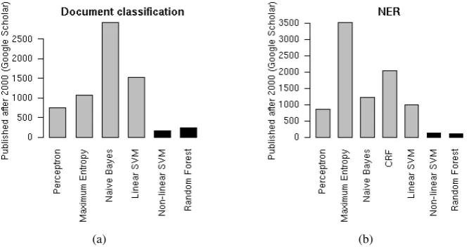
(a) (b)
Figure 1: Classifier models used for a) document classification and b) named entity recognition. Linear models are represented with gray bars and non-linear models with black.
cally list of all features (with parameters), such as for example n-grams (nis a parameter), con-text of words, part of speech, lemmas, stems, etc. Owing to the very large number of features, lin-ear (or log-linlin-ear) classifiers are preferred, because they are robust and can be trained fast. Simple search in Google Scholar shows that most fre-quently used models for document classification are Naive Bayes, linear SVMs (Cortes and Vapnik, 1995), Perceptrons (Rosenblatt, 1957) and Max-imum Entropy (Berger et al., 1996) (Figure 1a). In contrast, non-linear models such as non-linear SVMs and Random Forest (Breiman, 2001) and Classification trees (Breiman et al., 1984) are sig-nificantly under-represented. For Named Entity Recognition, Maximum Entropy and CRFs (Laf-ferty, 2001) are mostly used, but other linear mod-els like Perceptron, Naive Bayes and linear SVMs are employed (Figure 1b). Non-linear models are significantly less frequent. Feature induction can be used to efficiently introduce non-linearity in large models, in the form of feature conjunctions. As the space of all conjunctions of arbitrary length is very large (2#features), a greedy search
ap-proach is applied for selecting the most promis-ing conjunctions with reasonable computational cost. In (McCallum, 2003), a method for induc-ing features and conjunctions especially tailored to CRF models is proposed. Iteratively, the most promising feature or conjunction to be added to the model is identified. To this end, a gain func-tion is defined, for evaluating the improvement of the likelihood target upon the addition of the fea-ture. Conjunctions are considered only among the
top scoring feature candidates and the features al-ready included in the model. In (Vens and Costa, 2011), the authors use random forests to form fea-ture conjunctions, by traversing the trees from the root to the leaves.
In this article we present a method for feature selection and feature induction. The strengths of our method are fast running time and generality, in the sense that it can be used as preprocessing step to any classifier the user may choose.
2 Methods
Given are N pairs of observations and labels
(X1, Y1),(X2, Y2), ...,(XN, YN). The
observa-tionsXi are over a set of pbinary predicates (or
terms) T1, ..., Tp, which we call atomic features. For example, an atomic feature is an indicator of presence or absence of a particular word in a doc-ument. The class label can take the values from the set {c1, c2, ..., cK}. In this article. we use the notion of ‘features’ to denote predicates, and not the classical feature functionsf(Xi, ci) com-monly used in NLP tasks. The reason is that we wish to be consistent with the established no-tions of ‘feature selection’ and ‘feature induction’, which otherwise would have to be called ‘predi-cate selection’ and ‘predi‘predi-cate induction’.
The purpose of our method is to find a set of fea-tures consisting of atomic feafea-tures or conjunctions of atomic features which can predict the class vari-able with high accuracy. The classification model is the user’s choice.
Fisher test
Fisher’s exact test (Fisher, 1928) is used to exam-ine the significance of association between two bi-nary variables. We apply it to the contingency ta-ble between featureT and class indicatorYi and
retrieve the significance p-value, which expresses the probability of the observed values of the table under the assumption of independence between the variables. If the probability is very small (i.e. p-value is small), then the independence assump-tion is rejected. We define the Fisher test score for feature selection as: FT(T, Yi) = 1−p-value.
FT(T, Yi) always has values between0and1. A typical threshold for significance isp-value<0.05
or, more conservatively,p-value<0.01.
2.2 Induction (generating conjunctions)
We include in the model feature conjunctions of maximum lengthm, which is a parameter of our method. At each iteration, the conjunctions are formed between atomic features that exceed some relevance threshold and any other feature or con-junction still present in the list of features.
Before adding a conjunction Ti&Tj to the the
set Φ, we check if it has not been introduced al-ready, for example asTj&Ti. If at a certain step all conjunctions that are generated are already in
Φ, the algorithm stops (see step 8, Algorithm 1). In typical applications, it is unlikely that very long conjunctions have a great impact on the clas-sification performance. Therefore we suggest that
mis kept small in practice, a value up to3should be sufficient for most applications.
2.3 Complexity of the algorithm
As we already argued in the introduction, com-putational complexity is one important bottleneck of feature selection and induction algorithms. De-spite this, our method is fast. We run once through all samples in order to build the necessary data structures for evaluation of MI, IG, SU and FT scores, which takes O(pKN) time. The data structures esentially store the counts of samples in each class, for each feature. Thereafter, the complexity of scoring the set ofpfeatures and the sorting take place inO(pK)time, which is runm
times. The overall time is thusO(pKm+pKN), which isO(pKN), in most applications. In prac-tice the algorithm can become even faster by using sparse vectors to represent features.
2.4 Model training and evaluation
We use the FITSI Algorithm for generating a setΦ
of atomic features and conjunctions of length up to
m= 2. We use these features to represent the data and train a model M, which in our experiments can be a Perceptron or a Naive Bayes model. The performance of the algorithm clearly depends on the parameters used for the feature induction and selection:σ,kandl.
If we exclude the scoring measureσ, which can be chosen by the user based on some subjective criteria, our algorithm has two numerical hyper parameters that can be estimated from data, in a way that the resulting model has optimal perfor-mance. We use B-fold cross-validation for this purpose. We first split the data into two subsets, for parameter selection and for testing. The part that is used for parameter selection is split into
B bins (5 in our experiments). For each combi-nation of parameters, we useB −1bins for fea-ture induction and model training and we evaluate the performance of the classifier on the remain-ing bin. In consequence, for each combination of parameters, a set ofB performance estimates are obtained, which allows to compute mean and stan-dard deviation. We identify the model with largest mean performance and select the simplest model (smallestk) that has the mean within one standard deviation from the best model. This is known as the one-standard-error rule, proposed by (Breiman et al., 1984). The parameters of this model are the optimal parameterskoptandlopt. We test this
model on the excluded samples and report a test performance.
We compare the performance of our model to that of a baseline model. To this end, we repeat the cross validation described above, but we do not perform any feature induction.
For evaluating the performance of a classifier, we use the F1 measure, which is the harmonic mean of precision and recall.
3 Data
PA data: The ”PA” dataset was developed by the Press Association1 to enable the implemen-tation of a system for recognition and seman-tic disambiguation of named entities in press re-leases. Given certain metadata for a number of overlapping candidate entities, an array of fea-tures derived from the textual context of their
currence, and additional document-level metadata, the model recognizes which (if any) of the candi-date entities is the one referenced in the text.
The corpus is annotated with respect to peo-ple, organization and location mentions; a special ”negative” label denotes the candidates that can be considered irrelevant in the given context. In all cases, at most one of the overlapping candidates is annotated as positive. The dataset comprises a total of2539manually curated documents, and a total of85602concept mentions (this number rep-resents the total of all candidate instances, includ-ing those annotated as non-entities).
For this dataset, the domain of the press releases is an important factor during classification, and specific features that express the belonging of a press release to a particular domain or category are also available. The dataset comprises articles from two domains: ”General News” and ”Olympics”.
We remove non-location entity candidates, thus reducing the problem to the binary classification task of discerning locations from non-entities. We split the corpus into a training set (2369 docu-ments) and a held-out test set (160documents). As a result of this preprocessing, we have 2 classes (Location and Negative), 46273 instances, and a target to irrelevant instance counts ratio of0.17.
From the training document set, we extracted
50455atomic features.
As performance measure we report the F1 score of the positive class (i.e. ‘Location’).
4 Results
We performed feature induction using in turn all the measures of feature relevance mentioned in Section 2.1, followed by training Naive Bayes and Perceptron classifiers. The parameters k and l
(l > k) of the feature induction step were itera-tively selected from the set:
{0.1%,0.25%,0.5%,0.75%,1%,2.5%,5%,7.5%,10%,25%}
of the total number of featuresp.
We used 5-fold cross-validation for selection of the optimal parameters kopt and lopt, as ex-plained in section 2.4. Figure 2 illustrates the cross-validation search grid for the particular com-bination of feature induction with MI score and a Perceptron classifier. The intensity of the shade of gray is proportional to the average F1 mea-sure over the 5folds. The standard deviation for each combination of parameters is not shown in
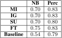
Figure 2:Parameter grid search by cross-validation.
NB Perc MI 0.70 0.83
IG 0.70 0.83
SU 0.70 0.80
FT 0.75 0.83
Baseline 0.54 0.79
Table 1: Performance on the test dataset of classification models using various measures of feature relevance and com-parison with the baseline.
the image. The largest average F1 is0.825and is achieved for k = 25% andl = 0.75%of p.The standard deviation of this model is 0.009, esti-mated based on the 5 cross-validation folds. A simpler model, with k = 25% and l = 0.1%
has average performance of0.824, which is within one standard deviation from the maximum perfor-mance, hence there is no statistically significant difference between the two models. We thus chose the simpler model as optimal.
In Table 1, we show the performance of the optimal models (determined by cross validation). The models that we investigated are various com-binations of feature scoring measures (as rows) and classifiers (as columns). We compare to a Baseline model (last row), which is either a Naive Bayes or Perceptron, without any feature induc-tion. Clearly, all our models outperform the Base-line, by a large margin: up to20%in the case of Naive Bayes models and up to4%for Perceptrons. In general, Naive Bayes classifiers are worse than the Perceptron. Fisher test ranking appears to work best for Naive Bayes classifiers, whereas for Perceptron models achieve similar performance for most of the scoring measures (apart from Sym-metrical Uncertainty).
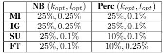
NB(kopt, lopt) Perc(kopt, lopt) MI 25%,0.25% 25%,0.1%
IG 25%,0.25% 25%,0.1%
SU 25%,0.1% 10%,0.1%
FT 25%,0.1% 10%,0.25%
Table 2:Parameters of the resulting models.
validation. In general many atomic features are included in the model, indicated by the large val-ues ofkopt, which are in general25%. Only two models select 10% features, namely the Percep-tron with FT and SU. The most common values forloptare0.25%and0.1%, which means that the useful conjunctions are those that comprise at least one high scoring atomic feature (from top0.01%
or0.25%). In contrast, a larger lopt would mean that the model benefits from conjunctions between two low scoring atomic features, which is not the case, according to our results.
5 Analysis of conjunctions
The purpose of feature induction is to generate useful combinations of features without the help of an expert in the domain of the application. Below we comment on interesting (types) of conjunctions that rank high ccording to the Perceptron model using the MI criterion for feature ranking, which showed highest performance.
- http://www.geonames.org/ontology#P.PPLC & ANNIES=location˙city
The Geonames ontology2 indicates that the candidate is a capital and Gate’s ANNIE3 suggests that the instance is a city. Therefore, the conjunction reinforces the recommenda-tion for a locarecommenda-tion. The conjuncrecommenda-tion is very informative.
- PrevWord = ”in” & MOST˙PROBABLE=true
If the word preceding the candidate is ‘in’ and Location is most probable label of the entity, then there is a strong indication that the entity is indeed a Location.
- PrevWord = ”in” & NoCandidates=1
The conjunction between previous word be-ing ‘in’ and the absence of other candidates at the specific location is a strong indicator for Location. This is a linguistic pattern that most experts would add to the model. Our al-gorithm automatically generates this pattern.
2
www.geonames.org
3http://gate.ac.uk/
- ANNIES=location˙country & pacategory:Olympics
A very interesting domain-specific conjunc-tion is formed by the indicaconjunc-tion of ANNIE to a country and the category of the docu-ment being Olympics. Even though ANNIE points to a country, the fact that the document belongs to the Olympics category makes the Location less likely, because the candidate is most probably referring to a team. Such conjunctions are specific to domain adapta-tion tasks and our algorithm generates it auto-matically, without defining a domain adapta-tion problem explicitly. Only adding atomic domain features allows for generating of do-main specific-conjunctions.
- multiple conjunctions including the domain name
Our algorithm ranks high various conjunc-tions that include the domain of the docu-ment. As commented already above, our ap-proach seems to implicitly perform domain adaptation, by adding conjunctions between features that play different roles in different domains and the respective domain features (very similar to the approach of (Daum´e, 2009)).
6 Discussion
We introduced a greedy heuristic for feature se-lection and induction. The method is applied as a preprocessing step, prior to model fitting, there-fore it is independent from the classifier chosen by the user. It is very fast in practice, having all the advantages of the filter-based methods over com-plex wrappers and embedded methods.
We applied the method on a custom dataset from Press Association, for named entity disam-biguation. In particular, we recognized Locations from negative entities. The results, presented in the form of F1 measure corresponding to the Loca-tion class, show great improvements over the base-line.
References
Adam L. Berger, Vincent J. Della Pietra, and Stephen A. Della Pietra. 1996. A maximum entropy ap-proach to natural language processing. Comput. Linguist., 22(1):39–71.
Leo Breiman, Jerome Friedman, Charles J. Stone, and R. A. Olshen. 1984. Classification and Regression Trees. Chapman and Hall/CRC.
Leo Breiman. 2001. Random forests. Machine Learn-ing, 45(1):5–32.
Corinna Cortes and Vladimir Vapnik. 1995. Support-vector networks. Machine Learning, 20(3):273– 297.
H. Daum´e. 2009. Frustratingly easy domain adapta-tion. CoRR, abs/0907.1815.
Asif Ekbal, Sriparna Saha, Olga Uryupina, and Mas-simo Poesio. 2011. Multiobjective simulated annealing based approach for feature selection in anaphora resolution. InDAARC, pages 47–58.
R.A. Fisher. 1928. Statistical methods for research workers. Oliver and Boyd.
George Forman. 2003. An extensive empirical study of feature selection metrics for text classification. J. Mach. Learn. Res., 3:1289–1305.
Isabelle Guyon and Andr´e Elisseeff. 2003. An intro-duction to variable and feature selection. J. Mach. Learn. Res., 3:1157–1182.
Patrick Haffner, Steven J. Phillips, and Robert E. Schapire. 2005. Efficient multiclass implementa-tions of l1-regularized maximum entropy. CoRR, abs/cs/0506101.
Richard W. Hamming. 1986. Coding and Information Theory. Prentice-Hall, Inc., Upper Saddle River, NJ, USA.
Noppadon Kamolvilassatian. 2002. Property-based feature engineering and selection. Master’s the-sis, Department of Computer Sciences, University of Texas at Austin.
Ron Kohavi and George H. John. 1997. Wrappers for feature subset selection. Artificial Intelligence, 97(1–2):273–324.
John Lafferty. 2001. Conditional random fields: Prob-abilistic models for segmenting and labeling se-quence data. pages 282–289. Morgan Kaufmann.
Changki Lee and Gary Geunbae Lee. 2006. In-formation gain and divergence-based feature selec-tion for machine learning-based text categorizaselec-tion. (1):155–165.
Chang-Hwan Lee, Fernando Gutierrez, and Dejing Dou. 2011. Calculating feature weights in naive bayes with kullback-leibler measure. In Proceed-ings of the 2011 IEEE 11th International Conference on Data Mining, ICDM ’11, pages 1146–1151.
David D. Lewis. 1992. Feature selection and feature extraction for text categorization. In Proceedings of Speech and Natural Language Workshop, pages 212–217. Morgan Kaufmann.
Andrew McCallum. 2003. Efficiently inducing fea-tures of conditional random fields.
A Moh’d A Mesleh. 2007. Chi square feature extrac-tion based svms arabic language text categorizaextrac-tion system.
P. M. Narendra and K. Fukunaga. 1977. A branch and bound algorithm for feature subset selection. IEEE Trans. Comput., 26(9):917–922.
F. Rosenblatt. 1957. The Perceptron, a Perceiving and Recognizing Automaton Project Para. Cornell Aeronautical Laboratory report.
Karl-Michael Schneider. 2004. A new feature selec-tion score for multinomial naive bayes text classifi-cation based on kl-divergence. InProceedings of the ACL 2004 on Interactive poster and demonstration sessions, ACLdemo ’04.
Hirotoshi Taira and Masahiko Haruno. 1999. Feature selection in svm text categorization. InProceedings of the AAAI ’99, pages 480–486.
Harun Uguz. 2011. A two-stage feature selection method for text categorization by using information gain, principal component analysis and genetic al-gorithm. Knowledge-Based Systems, 24(7):1024– 1032.
Celine Vens and Fabrizio Costa. 2011. Random forest based feature induction. InICDM, pages 744–753.
Jihoon Yang and Vasant Honavar. 1998. Feature subset selection using a genetic algorithm. IEEE Intelligent Systems, 13(2):44–49.