A Simple and Efficient Method to Generate Word Sense Representations
Luis Nieto Pi˜na and Richard Johansson
Spr˚akbanken, Department of Swedish, University of Gothenburg Box 200, SE-40530 Gothenburg, Sweden
{luis.nieto.pina, richard.johansson}@svenska.gu.se
Abstract
Distributed representations of words have boosted the performance of many Natu-ral Language Processing tasks. However, usually only one representation per word is obtained, not acknowledging the fact that some words have multiple meanings. This has a negative effect on the individ-ual word representations and the language model as a whole. In this paper we present a simple model that enables recent tech-niques for building word vectors to rep-resent distinct senses of polysemic words. In our assessment of this model we show that it is able to effectively discriminate between words’ senses and to do so in a computationally efficient manner.
1 Introduction
Distributed representations of words have helped obtain better language models (Bengio et al., 2003) and improve the performance of many natural language processing applications such as named entity recognition, chunking, paraphrasing, or sentiment classification (Turian et al., 2010; Socher et al., 2011; Glorot et al., 2011). Recently, the Skip-gram model (Mikolov et al., 2013a; Mikolov et al., 2013b) was proposed, which is able to produce high-quality representations from large collections of text in an efficient manner.
Despite the achievements of distributed repre-sentations, polysemy or homonymy are usually disregarded even when word semantics may have a large influence on the models. This results in several distinct senses of one same word sharing a representation, and possibly influencing the repre-sentations of words related to those distinct senses under the premise that similar words should have similar representations. Some recent attempts to address this issue are mentioned in the next sec-tion.
We present a simple method for obtaining sense representations directly during the Skip-gram training phase. It differs from most previ-ous approaches in that it does not need to create or maintain clusters to discriminate between senses, leading to a significant reduction in the model’s complexity. It also uses a heuristic approach to determining the number of senses to be learned per word that allows the model to use knowledge from lexical resources but also to keep its ability to work withouth them. In the following sections we look at previous work, describe our model, and in-spect its results in qualitative and quantitative eval-uations.
2 Related Work
One of the first steps towards obtaining word sense embeddings was that by Reisinger and Mooney (2010). The authors propose to cluster occur-rences of any given word in a corpus into a fixed number K of clusters which represent different word usages (rather than word senses). Each word’s is thus assigned multiple prototypes or em-beddings.
Huang et al. (2012) introduced a neural lan-guage model that leverages sentence-level and document-level context to generate word embed-dings. Using Reisinger and Mooney (2010)’s ap-proach to generate multiple embeddings per word via clusters and training on a corpus whose words have been substituted by its associated cluster’s centroid, the neural model is able to learn multi-ple embeddings per word.
Neelakantan et al. (2014) tried to expand the Skip-gram model (Mikolov et al., 2013a; Mikolov et al., 2013b) to produce word sense embeddings using the clustering approach of Reisinger and Mooney (2010) and Huang et al. (2012). No-tably, Skip-gram’s architecture allows the model to, given a word and its context, select and train a word sense embedding jointly. The authors
also introduced anon-parametricvariation of their model which allows a variable number of clusters per word instead of a fixedK.
Also based on the Skip-gram model, Chen et al. (2014) proposed to maintain and train con-text word and word sense embeddings conjunctly, by training the model to predict both the context words and the senses of those context words given a target word. To avoid using cluster centroids to represent senses, the number of sense embeddings per word and their initial values are obtained from a knowledge network.
Our system for obtaining word sense embed-dings also builds upon the Skip-gram model (which is described in more detail in the next sec-tion). Unlike most of the models described above, we do not make use of clustering algorithms. We also allow each word to have its own number of senses, which can be obtained from a dictionary or using any other heuristic suitable for this purpose. These characteristics translate into a) little over-head calculations added on top of the initial word-based model; andb) an efficient use of memory, as the majority of words are monosemic.
3 Model Description
3.1 From Word Forms to Senses
The distributed representations for word forms that stem from a Skip-gram (Mikolov et al., 2013a; Mikolov et al., 2013b) model are built on the premise that, given a certain target word, they should serve to predict its surrounding words in a text. I.e., the training of a Skip-gram model, given a target wordw, is based on maximizing the log-probability of the context words ofw,c1, . . . , cn:
n X
i=1
logp(ci|w). (1)
The training data usually consists of a large col-lection of sentences or documents, so that the role of target word w can be iterated over these se-quences of words, while the context wordsc con-sidered in each case are those that surround w
within a window of a certain length. The objec-tive then becomes maximizing the average sum of the log-probabilities from Eq. 1.
We propose to modify this model to include a sensesof the wordw. Note that Eq. 1 equals
logp(c1, . . . , cn|w) (2)
if we assume the context wordsci to be
indepen-dent of each other given a target wordw. The no-tation in Eq. 2 allows us to consider the Skip-gram as a Na¨ıve Bayes model parameterized by word embeddings (Mnih and Kavukcuoglu, 2013). In this scenario, including a sense would amount then to adding a latent variables, and our model’s be-haviour given a target wordwis to select a senses, which is in its turn used to predictncontext words
c1, . . . , cn. Formally:
p(s, c1, . . . , cn|w) = p(s|w)·p(c1, . . . , cn|s) = p(s|w)·p(c1|s). . . p(cn|s).
(3)
Thus, our training objective is to maximize the sum of the log-probabilities of context words c
given a sensesof the target wordwplus the log-probability of the sensesgiven the target word:
logp(s|w) +
n X
i=1
logp(ci|s). (4)
We must now consider two distinct vocabular-ies:V containing all possible word forms (context and target words), and S containing all possible senses for the words inV, with sizes|V|and|S|, resp. Given a pre-setD∈N, our ultimate goal is to obtain|S|dense, real-valued vectors of dimen-sionDthat represent the senses in our vocabulary
S according to the objective function defined in Eq. 4.
The neural architecture of the Skip-gram model works with two separate representations for the same vocabulary of words. This double represen-tation is not motivated in the original papers, but it stems fromword2vec’s code1 that the model builds separate representations for context and tar-get words, of which the former constitute the ac-tual output of the system. (A note by Goldberg and Levy (2014) offers some insight into this sub-ject.) We take advantage of this architecture and use one of these two representations to contain senses, rather than word forms: as our model only uses target wordswas an intermediate step to se-lect a senses, we only do not need to keep a repre-sentation for them. In this way, our model builds a representation of the vocabularyV, for the context words, and another for the vocabularySof senses, which contains the actual output. Note that the
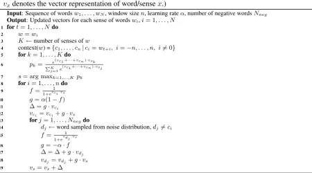
inter-Algorithm 1: Selection of senses and training using Skip-gram with Negative Sampling. (Note that
vxdenotes the vector representation of word/sensex.)
Input: Sequence of wordsw1, . . . , wN, window sizen, learning rateα, number of negative wordsNneg
Output: Updated vectors for each sense of wordswi,i= 1, . . . , N
1 fort= 1, . . . , Ndo
2 w=wi
3 K←number of senses ofw
4 context(w) ={c1, . . . , cn|ci=wt+i, i=−n, . . . , n, i6= 0}
5 fork= 1, . . . , Kdo
6 pk= e
(vc1 +···+vcn)·vsk
PK
j=1e(vc1 +···+vcn)·vsj
7 s= arg maxk=1,...,K pk
8 fori= 1, . . . , ndo 9 f= 1+evci1 ·vs
10 g=α(1−f)
11 ∆ =g·vci 12 vci =vci+g·vs 13 forj= 1, . . . , Nnegdo
14 dj←word sampled from noise distribution,dj6=ci
15 f= 1
1+evdj·vs
16 g=−α·f
17 ∆ = ∆ +g·vdj 18 vdj =vdj+g·vs
19 vs=vs+ ∆
Compounds have been segmented automatically and when a lemma was not listed in SALDO, we used the parts of the compounds instead. The input to the software computing the embeddings con-sisted of lemma forms with concatenated part-of-speech tags, e.g.dricka-verb for the verb ‘to drink’ anddricka-noun for the noun ‘drink’.
The training time of our model on this corpus was 22 hours. For the sake of time performance comparison, we run an off-the-shelf word2vec
execution on our corpus using the same parameter-ization described above; the training of word vec-tors took 20 hours, which illustrates the little com-plexity that our model adds to the original Skip-gram.
4.1 Inspection of nearest neighbors
We evaluate the output of the algorithm qualita-tively by inspecting the nearest neighbors of the senses of a number of example words, and com-paring them to the senses listed in SALDO.
Table 1 shows the nearest neighbor lists of the senses of two words where the algorithm has been able to learn the distinctions used in the lexicon. The verb flyga ‘to fly’ has two senses listed in SALDO: to travel by airplane and to move through the air. The adjective ¨om ‘tender’ also has two senses, similar to the corresponding English word: one emotional and one physical. The lists are se-mantically coherent, although we note that they
are topical rather than substitutional; this is ex-pected since the algorithm was applied to lemma-tized and compound-segmented text and we use a fairly wide context window.
flyg‘flight’ flaxa‘to flap wings’ flygning‘flight’ studsa‘to bounce’ flygplan‘airplane’ sv¨ava‘to hover’ charterplan‘charter plane’ skjuta‘to shoot’ SAS-plan‘SAS plane’ susa‘to whiz’
(a)flyga‘to fly’
k¨arleksfull‘loving’ svullen‘swollen’ ¨omsint‘tender’ ¨omma‘to be sore’ smek‘caress’ v¨arka‘to ache’ k¨arleksord‘word of love’ m¨orbulta‘to bruise’ ¨omt˚alig‘delicate’ ont‘pain’
(b)¨om‘tender’
Table 1: Examples of nearest neighbors of the two senses of two example words.
In a related example, Figure 1 shows the projec-tions onto a 2D space3 of the representations for the two senses of ˚asna: ’donkey’ or ’slow-witted person’, and those of their corresponding nearest neighbors.
For some other words we have inspected, we fail to find one or more of the senses. This is typ-ically when one sense is very dominant, drowning out the rare senses. For instance, the word rock
åsna-1 mulåsna(mule)
kamel(camel) tjur(bull) får(sheep) lama(llama)
åsna-2 idiot dummer(fool)
fåne(jerk) tönt(dork)
fårskalle(muttonhead)
Figure 1: 2D projections of the two senses of ˚asna(’donkey’ and ’slow-witted person’) and their nearest neighbors.
has two senses, ‘rock music’ and ‘coat’, where the first one is much more frequent. While one of the induced senses is close to some pieces of clothing, most of its nearest neighbors are styles of music.
In other cases, the algorithm has come up with meaningful sense distinctions, but not exactly as in the lexicon. For instance, the lexicon lists two senses for the nounb¨ona: ‘bean’ and ‘girl’; the al-gorithm has instead created two bean senses: bean as a plant part or bean as food. In some other cases, the algorithm finds genre-related distinc-tions instead of sense distincdistinc-tions. For instance, for the verb ¨alska, with two senses ‘to love’ or ‘to make love’, the algorithm has found two stylis-tically different uses of the first sense: one stan-dard, and one related to informal words frequently used in social media. Similarly, for the noun svamp ‘sponge’ or ‘mushroom’/‘fungus’, the al-gorithm does not find the sponge sense but distin-guishes taxonomic, cooking-related, and nature-related uses of the mushroom/fungus sense. It’s also worth mentioning that when some frequent foreign word is homographic with a Swedish word, it tends to be assigned to a sense. For in-stance, for the adjectivesur‘sour’, the lexicon lists one taste and one chemical sense; the algorithm conflates those two senses but creates a sense for the French preposition.
4.2 Quantitative Evaluation
Most systems that automatically discover word senses have been evaluated either by clustering the instances in an annotated corpus (Manandhar et al., 2010; Jurgens and Klapaftis, 2013), or by mea-suring the effect of the senses representations in a downstream task such as contextual word
similar-ity (Huang et al., 2012; Neelakantan et al., 2014). However, Swedish lacks sense-annotated corpora as well as word similarity test sets, so our evalua-tion is instead based on comparing the discovered word senses to those listed in the SALDO lexi-con. We selected the 100 most frequent two-sense nouns, verbs, and adjectives and used them as the test set.
To evaluate the senses discovered for a lemma, we generated two sets of word lists: one derived from the lexicon, and one from the vector space. For each sense si listed in the lexicon, we
cre-ated a listLi by selecting theN senses (for other
words) most similar tosi according to the
graph-based similarity metric by Wu and Palmer (1994). Conversely, for each sense vectorvjin our
vector-based model, a list Vj was built by selecting the N vectors most similar to vj, using the cosine
similarity. We finally mapped the senses back to their corresponding lemmas, so that the two sets
L = {Li}andV = {Vj}of word lists could be
compared.
These lists were then evaluated using standard clustering evaluation metrics. We used three dif-ferent metrics:
• Purity/Inverse-purity F-measure (Zhao and Karypis, 2001), where each of the lexicon-based listsLi is matched to the vector-based
list Vj that maximizes the F-measure, the
harmonic mean of the cluster-based precision and recall:
P(Vj, Li) = |V|jC∩jL|i| R(Vj, Li) = |V|jL∩iL|i|
The overall F-measure is defined as the weighted average of individualF-measures:
F =X
i
|Li| P
k|Lk|maxj F(Vj, Li)
• B-cubed F-measure (Bagga and Baldwin, 1998), which computes individual precision and recall measures for every item occurring in one of the lists, and then averaging all pre-cision and recall values. The F-measure is the harmonic mean of the averaged precision and recall.
• V-measure (Rosenberg and Hirschberg,
relative reduction of entropy in V when adding the information aboutL:
h(V, L) = 1−H(V|L)
H(V) Conversely, the completeness is defined
c(V, L) = 1−HH(L(L|V)).
Both measures are set to 1 if the denominator is zero.
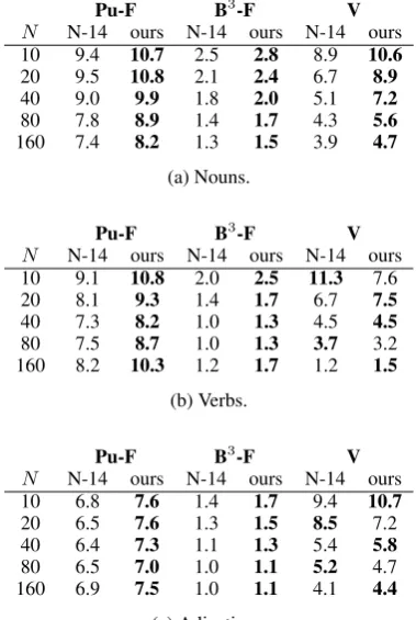
Table 2 shows the results of the evaluation for nouns, verbs, and adjectives, and for different val-ues of the list size N. As a strong baseline, we also include an evaluation of the sense represen-tations discovered by the system of Neelakantan et al. (2014), run with the same settings as our system. This system is available only in its para-metric version. (I.e., the number of senses per word is a fixed parameter.) As the words used in the experiments always have two senses as-signed, this parameter is set to 2. This accounts for fairness in the comparison with our approach, which is given theright number of senses by the lexicon (and thus in this case also 2). We used the three metrics mentioned above: Purity/Inverse-purity F-measure (Pu-F), B-cubed F-measure (B3
-F), and V-measure (V). As we can see, our sys-tem achieves higher scores than the baseline in al-most all the evaluations, despite using a simpler algorithm that uses less memory. Only for theV -measure the result is inconclusive for verbs and adjectives; for nouns, and for the other two evalu-ation metrics, our system is consistently better.
5 Conclusions and Future Work
In this paper, we present a model for automat-ically building sense vectors based on the Skip-gram method. In order to learn the sense vectors, we modify the Skip-gram model to take into ac-count the number of senses of each target word. By including a mechanism to select the most prob-able sense given a target word and its context, only slight modifications to the original training algo-rithm are necessary for it to learn distinct repre-sentations of word senses from unstructured text.
To evaluate our model we train it on a 1-billion-word Swedish corpus and use the SALDO lexi-con to inform the number of senses associated to each word. Over a series of examples in which we
Pu-F B3-F V
N N-14 ours N-14 ours N-14 ours 10 9.4 10.7 2.5 2.8 8.9 10.6
20 9.5 10.8 2.1 2.4 6.7 8.9
40 9.0 9.9 1.8 2.0 5.1 7.2
80 7.8 8.9 1.4 1.7 4.3 5.6
160 7.4 8.2 1.3 1.5 3.9 4.7
(a) Nouns.
Pu-F B3-F V
N N-14 ours N-14 ours N-14 ours 10 9.1 10.8 2.0 2.5 11.3 7.6 20 8.1 9.3 1.4 1.7 6.7 7.5
40 7.3 8.2 1.0 1.3 4.5 4.5
80 7.5 8.7 1.0 1.3 3.7 3.2 160 8.2 10.3 1.2 1.7 1.2 1.5
(b) Verbs.
Pu-F B3-F V
N N-14 ours N-14 ours N-14 ours 10 6.8 7.6 1.4 1.7 9.4 10.7
20 6.5 7.6 1.3 1.5 8.5 7.2 40 6.4 7.3 1.1 1.3 5.4 5.8
80 6.5 7.0 1.0 1.1 5.2 4.7 160 6.9 7.5 1.0 1.1 4.1 4.4
(c) Adjectives.
Table 2: Evaluation of the senses produced by our system and that of Neelakantan et al. (2014).
analyse the nearest neighbors of some of the rep-resented senses, we show how the obtained sense representations are able to replicate the senses de-fined in SALDO, or to make novel sense distinc-tions in others. On instances in which a sense is dominant we observe that the obtained represen-tations favour this sense in detriment of less com-mon ones.
Language Processing and Computational Natural Language Learning (EMNLP-CoNLL), pages 410– 420, Prague, Czech Republic.
Richard Socher, Eric H Huang, Jeffrey Pennin, Christo-pher D Manning, and Andrew Y Ng. 2011. Dy-namic pooling and unfolding recursive autoencoders for paraphrase detection. InAdvances in Neural In-formation Processing Systems, pages 801–809. Joseph Turian, Lev Ratinov, and Yoshua Bengio. 2010.
Word representations: a simple and general method for semi-supervised learning. InProceedings of the 48th Annual Meeting of the Association for Compu-tational Linguistics, pages 384–394. Association for Computational Linguistics.
Zhibiao Wu and Martha Palmer. 1994. Verb seman-tics and lexical selection. In Proceedings of the 32nd Annual Meeting of the Association for Com-putational Linguistics, pages 133–138, Las Cruces, United States.