Long Term Forecasting of Solar Power Using Artificial Neural Network

(1)

CSEIT1846148 | Published – 08 May 2018 | May-June 2018 [ (4 ) 6 : 775-782 ]

National conference on Engineering Innovations and Solutions (NCEIS – 2018)

775

Long Term Forecasting of Solar Power Using Artificial Neural

Network

Harshitha

H V

1

, PG scholar

1

, Ms. Rekha C M

2

1_{Power systems Engineering, Department of EEE, Acharya Institute of Technology, Bangalore, Karnataka,}

India

2_{Assistant Professor, Department of EEE, Acharya Institute of Technology, Bangalore, Karnataka, India}

ABSTRACT

The rapid growth of solar Photovoltaic (PV) technology has been very visible over the past decade. Such increase in the integration of solar generation has brought attention to the forecasting issues. This paper presents a new approach to tackle the long-term forecasting challenge and accordingly reduce the uncertainty of the PV forecast, which would accordingly help facilitate its integration into the electric power grid. This paper presents a solar power forecasting using artificial neural networks (ANNs). The neural network structures, namely, feed forward back propagation (FFBP), have been used to forecast a photovoltaic panel output power and approximate the generated power. The neural networks have four inputs and one output. The inputs are solar radiation, ambient temperature, humidity and wind speed; the output is the Solar power. The data used in this paper started from January 1,2013 ,until December 31,2017. The five years of data were split into two parts: 2006–2008 and 2009 2010; the first part was used for training and the second part was used for testing the neural networks. A mathematical equation is used to estimate the generated power.

Keywords: Photovoltaic, Artificial neural network,solar forecasting.

I. INTRODUCTION

Variable energy generations, particularly from renewable energy resources such as wind and solar energy plants have created operational challenges for the electric power grid because of the uncertainty involved in their output in the short term. When the penetration level of the variable generation is high, the intermittency of these resources may adversely affect the operation of the electric grid. Thus, wherever the variable generation resources are used, it becomes highly desirable to maintain higher than normal operating reserves and efficient energy storage systems to manage the power balance in the

system. The operating reserves that use fossil fuel generating units should be kept as low as possible to get the highest benefit from the deployment of the variable generations [1]. Therefore, forecasting these renewable resources takes on a vital role in the operation of power systems and electricity markets.

II. RELATED WORK

(2)

existing approaches predict the solar irradiance and use it to estimate the power output (indirect prediction) but there are also some recent approaches that directly predict the PV power output. Inman et al. [4] reviewed methods for solar power forecasting and classified them into five main groups: statistical (regressive) methods (e.g. auto regressive, moving average, and combinations of them such as ARIMA, methods based on artificial intelligence techniques (e.g. NNs, nearest neighbor), numerical weather prediction methods, remote sensing methods (e.g. satellite and statistical satellite) and local sensing methods (e.g. sky-imager).

Pedro and Coimbra [5] predicted the solar power 1 and 2 hours ahead from a time series of previous solar power values only, without using any exogenous variables. They compared the performance of four methods: ARIMA, k nearest neighbor, NN trained with the backpropagation algorithm and NN trained with a genetic algorithm. They conducted an evaluation using data for two full years and found that the two NN based methods outperformed the other methods, and that the NN trained with the genetic algorithm prediction model. The two NN approaches obtained Mean Absolute Error (MAE) in the range of 42.96 - 61.92 kW for 1 hour ahead prediction and 62.53 - 87.76 kW for 2 hours ahead prediction for a 1 MW PV power plant.

Chen et al. [2] introduced a new approach for 1 to 24 hours ahead solar power prediction based on Radial Basis Function NN (RBFNN). At first, they categorized the days into sunny, cloudy and rainy using self-organizing map NNs and based on the weather predictions of solar irradiance and cloudiness. Then, a separate RBFNN prediction model for each group was trained to predict the 24 hourly PV power outputs for the next day.

Shi et al. [9] proposed a similar approach the days were clustered into four groups (clear-sky, cloudy,

and rainy) and a separate SVR prediction model was built for each group. The obtained Mean Relative Error (MRE) was between 4.85% (for sunny day) and 12.42% (for cloudy day).

Chow et al. [8] applied NNs for predicting the PV power output 10 and 20 minutes ahead. As inputs to the NNs they used solar irradiation, temperature, solar elevation angle and solar azimuth angle. They developed multi-layer perceptron with one hidden layer, trained with the backpropagation algorithm, with early stopping criterion based on validation set to avoid overtraining. The results were promising and showed that NNs can successfully model the nonlinear relationship between the meteorological parameters and the PV solar power output.

Mandal et al. [7] used wavelet transform in conjunction with RBFNNs. They firstly decomposed the highly fluctuating PV power time series data into multiple time-frequency components. The one hour ahead decomposed PV power output was then predicted using the decomposed components, as well as previous solar irradiation and temperature data. The final prediction was generated by applying the inversed wavelet transform. The results showed good accuracy, with the combination of wavelet transform and RBFNN outperforming RBFNN without wavelets.

Mellit et al. [6] presented a different wavelet based approach, called wavelet network. Instead of decomposing the data and applying NNs to predict each component, they used wavelets as activation functions in the NNs. The approach was effective, achieving Mean Absolute Percentage Error (MAPE) of about 6%.

(3)

evaluation showed that SVR was more accurate compared to ARIMA and RBFNN. Approaches based on fuzzy logic were also proposed.

Jararzadeh et al. in [13] investigated the application of interval type-2 Takagi-Sugeno-Kang fuzzy systems. Using temperature and solar irradiance as inputs, they predicted the output of PV plants under different operating conditions, and showed better results than ARIMA.

Yona et al. [3] proposed a hybrid approach by combing NNs and fuzzy theory. They first applied a fuzzy model to estimate the hourly insolation using different weather variables such as clouds, humidity and temperature. The output of the fuzzy model was then fed to a recurrent NN, to predict the hourly power output of the PV plant.

Yang et al. [11] integrated SOM, SVR, and fuzzy inference to develop a hybrid approach for one day ahead solar power prediction. SOM and SVR were applied to classify the historical input data and to develop the prediction model, respectively. The fuzzy inference was used to select the best model from a group of trained SVRs, depending on the available weather predictions. An evaluation using one year of solar data showed that the hybrid method outperformed NN and SVR.

III. STATISTICAL VARIABLE GENERATION

FORECASTING MODELS

Forecasting models are continuously being improved to generate more accurate forecasts of solar and wind power. In this section, the statistical models that use both non-learning and learning approaches are described.

A. Statistical Non-Learning Approach Models These models describe the connection between predicted solar irradiance from numerical weather predictions (NWP) and solar power production

directly by statistical analysis of time series from historical data without considering the physics of the system. This connection can be used for forecasts in the future plant outcomes. Plenty of regression models are already implemented as time-series forecasting models, some of which include autoregressive integrated moving averages (ARIMA), and multiple linear regression (MLR) analysis model [2] to name just two types.

B.Statistical Learning Approach Models

Artificial intelligence (AI) methods are used to learn the relationship between predicted weather conditions and the power output generated as historical time series. Unlike statistical approaches, AI methods use algorithms that are able to implicitly describe nonlinear and highly complex relationship between input data (NWP predictions) and output power instead of an explicit statistical analysis. For both the statistical and AI approaches, high quality time series data consisting of weather predictions and power outputs from the past are very important [3], [4]. One of the most common statistical learning models is the artificial neural network.

IV. PROPOSED APPROACHES

The ANN is loosely a simple biological analogy of the brain. They are implemented in widespread applications with different AI approaches such as supervised, unsupervised, and reinforcement learning approaches. In the supervised learning approach, the ANN learns from the data by training them to approximate and estimate the function or the relationship between the input and the output variables.

(4)

while attempting to minimize the errors by using an appropriate optimization technique such as the gradient descent method. After sufficient training iterations with known input data, the weights between the nodes are adjusted until they give a correct response. Then, the ANN will give the correct response to the (unknown) input data that it has never seen before. The ANN can learn to generalize in this fashion. More sophisticated algorithms are introduced for training ANNs with different optimization methods to improve the performance.

In this paper, ANN model uses the most widely used “vanilla” feed-forward neural networks, sometimes called the single hidden layer network. The ANN model is used as a nonlinear statistical tool to forecast solar power.

Multi-layered Perceptrons has been applied successfully to solve some difficult and diverse problems basing on a preliminary supervised training with error back propagation algorithm using an error correction learning rule. Basically, error back learning consists in two pass through the different layers of the network, a forward pass and backward pass. In the forward pass an activity pattern (input vector) is applied to the sensory nodes of the network, its effect propagates through the network layer by layer to produce an output as actual response.

Figure 1. Architecture graph of a MLPNN with 50 hidden layers

During the backward pass synaptic weights are adjusted in accordance to an error correction-rule. The error signal (subtracted from a desired value) is

then propagated backward through the network against the direction of the synaptic connections [9]. In general MLPNN’s can have several hidden layers (Figure 1), however according to K.M.Hornik [10] a neural network with single hidden layer is able to approximate a function of any complexity. If we consider a MLPNN with one hidden layer, tanh as an activation function and a linear output unit, the equation describing the network structure can be expressed as:

∑ ∑ ) (1)

Where is the output of the output unit,

and are the network weights, p is the number of

network inputs, and q is the number of hidden units. During the training process, weights are adjusted in such a way that the difference between the obtained outputs and the desired outputs is minimized, which is usually done by minimizing the following error function

E= ∑ ∑ (2)

Where r is the number of network outputs and n is the number of training examples. The minimization of the error function is usually done by gradient descent methods

The mean squared error (MSE) is used for evaluation of predictive power as follows;

MSE = ∑ ̅ (3)

Where ̅̅̅̅ is a vector of the 𝑁 prediction and is the vector of the real values.

V. THE DATA

A. Data Source

The data is derived from the Karnataka power Corporation Limited Shivanasamudram.

B. Data Description

(5)

are 4 independent variables, these are solar radiation, ambient temperature, humidity and wind speed.

A. Data Preparation

It is always a good idea to get the analysis of the historical data before setting up the forecasting model. The available historical data contains the solar power and 3 weather variables

Figure 2. Flowchart diagram of the solar forecasting modeling

The data preparation is an important step for treating the data to be ready for the analysis and modeling steps. The various steps of the data preparation are shown in Figure 2.

B. The Model Building

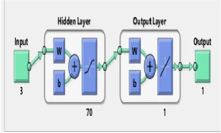
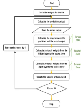
Themain steps of building the forecasting model are shown in Figure 3. MATLAB is used for building the ANN model as shown in Fig 4. It is a feed-forward curve fitting type, which works well when it is not necessary to use the past delayed values of the output as a feedback variable, also several available inputs are applied to extract a better regression. The ANN has the input layer, a hidden layer, and the output layer. The hidden layer has 70 nodes besides the bias node, which is feeding into every node in the hidden and output layers. The bias node is for shifting the activation function left or right, because sometimes the variation in the weights is not enough to minimize the errors and enhance the model performance.

Figure 3. Flowchart diagram for building the ANN model

Figure 4. Block diagram of the ANN topology.

When the predictor variables interact with each other and grouped in the ANN’s input layer, they could lose some of their correlation power. Therefore, in the total mix of selected variables, the best candidate model is needed. So every time a new weather variable is added as a new input to the existing list of inputs, the ANN must be run several times to calculate the MSE until the best group of input variables is found. By carrying out the three main steps of building the model, training, and testing to reduce the dimension of inputs variables, we arrive at the candidate model with most efficient performance.

The ANN model with 3 input variables was found to have the least MSE as shown in the Figure 6 An ANN model with a large number of input variables and nodes could lead to the overfitting issue, which is the situation where the model performs well in the training stage, but produces inaccurate forecasts in the testing stage. For the purpose of solar forecasting, we found the candidate model with 4 input variables to have the least MSE,the hidden layer of the ANN had 15 nodes.

(6)

2014. Keep in mind, the training of each case is carried out separately, May 2014 has more historical data than in September 2013 case. Next, an investigation of the ultimate performance of the model and comparisons with other models is done.

Multilayer feed-forward with backpropagation neural networks (MFFNNBP) is an MLPNN that passes the inputs and the weights from one layer to the next one through the feed forward process and then it performs the weights update to be back-propagated to the previous layers in order to recalculate the weight. In MLPNN, the output of a layer will be an input for the next layer passing from the input layer to the output layer; the equations used for this procedure are illustrated as follows:

Output = ∑ ) (4)

Where the output of the first hidden layer which calculated using the following expression:

= ∑ ) (5)

Where and are the activation functions for output layer and hidden layer, which calculated as in the following expressions:

= (6)

= x (7)

Where, x = input vector. Depending on equations above, the weights are updated use as the following expression:

(8)

Where µ is the learning rate (normally between 0 and 1).The final output depends on all earlier layer's output, weights, and the algorithm of learning used.

The backpropagation process calculates the gradient decent error between the desired and the predicted

output considering the new weights each time, this gradient is almost always used in a simple stochastic gradient descent algorithm to find the weights that minimize the error. Different algorithms are used for training the feed forward with backpropagation neural networks, which train the NN and reduce the error values by adjusting and updating the weights and the biases of the connections that form the neural network, two kinds of training algorithms are available to slow convergence according to steepest descent methods with better generalization, and fast convergence according to newton's method, but these

Figure 5. Flow chart of the FFBP model

(7)

VI. MODEL RESULTS AND EVALUATION

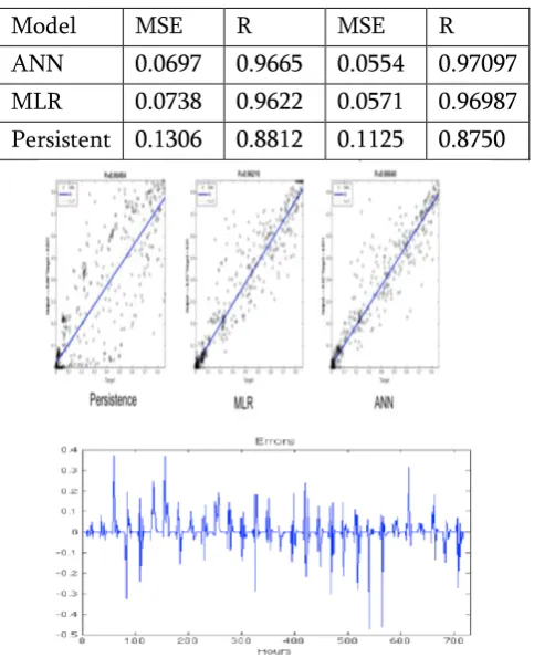
The following measures are used to evaluate the accuracy of the forecasts and the model performance plots and graphs, Mean Square Error (MSE), the correlation coefficient (R) between the forecasts and the actual measured solar power, and a comparison with other models. For comparison purposes, the Multiple Linear Regression (MLR) Analysis model [2], and the persistence forecasts model are used. The persistence model as its name implies, is obtained by keeping the actual solar power output at the current hour and using it as a solar power forecast for the next future hour.

The line plots are shown in Figure 6 for the actual solar power and its corresponding forecasts from ANN model and compared with MLR and persistence forecasts models. The day-ahead weather variables forecasts are used as input variables for the ANN and they are periodically generated and updated daily to forecast the next days. Therefore, the output of the forecasting model, which is the solar power forecasts, doesn’t change much by increasing the horizon time. The zoomed in plot on the right is for a sample day with a lower spike in the solar power generation. The forecasts from the ANN model have tracked the actual power better than the other models.

Figure 6. The line plots for actual solar power and the forecasts from ANN, MLR, and Persistence

models

As shown in Figure 7, the actual and the forecasts are plotted with residuals plot. The residuals plot has both positive and negative values. There appear to be many residuals of the ANN that are lying at or near

the zero value as shown on the top right plot which indicates that the generated forecasts are unbiased. The correlation coefficients R between the actual power and the forecasts for all models are also plotted. Table I summarizes the evaluation results of both test cases: September 2013 and May 2014 of the ANN and other model performance. It is obvious that the ANN outperforms other models. In addition, the May 2014 case has accurate forecasts because there are more historical data included in the training and validation stages of the model.

Table 1. The summary of Forecasts for both test months

Model MSE R MSE R

ANN 0.0697 0.9665 0.0554 0.97097 MLR 0.0738 0.9622 0.0571 0.96987 Persistent 0.1306 0.8812 0.1125 0.8750

Figure 7. The residuals plot of ANN model and the correlation coefficient plots for solar power forecasts

of ANN, MLR and Persistence models

(8)

Figure 8. shows the best validation performance is 2.9607 at epoch 4

VII. CONCLUSION

The artificial neural networks model outperforms the multiple linear regression analysis MLR model and the persistence model. The performance of the ANN depends on how well it is trained and on the quality of the data that is used. The feed-forward ANN with 3 weather variables and with step size for forecasts performed better than the other The residuals plot of ANN model and the correlation coefficient plots for solar power forecasts of ANN, MLR and Persistence models recursive neural networks. The normalized input data doesn’t improve the performance, but removing the night hours slightly improves the model performance. Plotting the data, investigating the correlation and sensitivity analysis between the variables, as well as data cleansing of outliers are essential data preparation steps before building the forecasting model. In the clear sky hours, the model produces more accurate forecasts than cloudy hours. The more accurate weather forecasts we use, the more accurate solar power forecasts will be produced. Using the classification variables and the interactions between the variables enhances the performance of the MLR model significantly but this is not the case for the ANN model. With additional historical data, the model performance will improve.

VIII. REFERENCES

1. A Botterud, J. Wang, V. Miranda, and R. J. Bessa, “Wind power forecasting in US electricity markets,” The Electricity Journal, vol. 23, no. 3, pp. 71–82, 2010.

2. M Abuella and B. Chowdhury, “Solar Power

Probabilistic Forecasting by Using Multiple Linear Regression Analysis,” in IEEE Southeastcon Proceedings, Ft. Lauderdale, FL, 2015.

3. M Lange and U. Focken, Physical Approach to

Short-Term Wind Power Prediction. Springer, 2006.

Elements of Statistical Learning, 2 Edition. Springer-Verlag New York, 2009.

6. J Kleissl, Solar Energy Forecasting and Resource

Assessment. Elsevier, 2013.

7. R H. Inman, H. T. C. Pedro, and C. F. M. Coimbra,

“Solar forecasting methods for renewable energy integration,” Prog. Energy Combust. Sci., vol. 39, no. 6, pp. 535–576, Dec. 2013.

8. “Global Energy Forecasting Competition 2014,

Probabilistic solar power forecasting.” [Online].

Available: http://www.crowdanalytix.com/

contests/global-energy-forecasting-competition-2014.

9. “Many fields have seconds in their units e.g.

radiation fields. How can instantaneous values be calculated?” [Online].

10. E. Lorenz, T. Scheidsteger, J. Hurka, D.

Heinemann, and C. Kurz, “Regional PV power prediction for improved grid integration,” Prog. Photovoltaics Res. Appl., vol. 19, no. 7, pp. 757– 771, 2011.

11. P. Mandal, S. T. S. Madhira, A. U. Hague, J. Meng,

and R. L. Pineda, "Forecasting power output of solar photovooltaic system using wavelet transform and artificial intelligence techniques," Procedia Computer Science, vol. 12, pp. 332-337, 2012. 12. S. K. Chow, E. W. Lee, and D. H. Li, "Short-term

prediction of photovoltaic energy generation by intelligent approach," Energy and Buildings, vol. 55, pp. 660-667, 2012.