Predicting U.S. business cycles with recurrent neural networks : An extensive multivariate time-series analysis for comparing LSTM and GRU networks

Turun kauppakorkeakoulu • Turku School of Economics

Subject Economics Date 23.6.2020

Author Markus Mäkelä Number of pages 103+appendices Title

Predicting U.S. business cycles with recurrent neural networks. An ex-tensive multivariate time-series analysis for comparing LSTM and GRU networks

Supervisor Prof. Jouko Vilmunen

Abstract

This study examines how 22 different long short-term memory (LSTM) and gated recurrent unit (GRU) network architectures suit predicting U.S. business cycles. The networks create 91-day forecasts for the dependent variable by using multivariate time-series data comprising 26

leading indicators’ values for the previous 400 days. The proposed models are evaluated by using a train-test split, where the proposed models are trained with data from 1980 to 2005, and the out-of-sample set consists of data between 2005 and 2015. The performance is evaluated by using mean squared error (MSE) and mean absolute error (MAE), and early warning signs are also considered beneficial.

The training algorithm consists of typical deep learning methods. MSE and L1 regulariza-tion are used for determining the cost, and minibatches of 32 examples are applied together with Nesterov accelerated momentum (NAG) learning algorithm. Early stopping is introduced to halt the training process when strong signs of overfitting are detected. Each proposed recur-rent neural network (RNN) architecture is trained three times, and these three networks’

aver-aged predictions are examined when comparing the architectures.

Performance-wise, a few LSTM networks stand out from the other proposed networks. Although the performance results favor the proposed LSTM networks slightly over their GRU equivalents, the difference is not substantial and, in turn, the proposed GRU networks offer less deviation in MSE and MAE between each architecture. However, these steadier performance results do not generate less volatile forecasts. Instead, the best performing networks and archi-tectures differentiate by offering less volatile predictions that also vary less from the real values.

Most of the models generate a considerable amount of early warning signs before the 2007 recession, which indicates their suitability for detecting turning points in business cycles. More-over, a wide range of the proposed LSTM and GRU network architectures learn the general pattern, also the smaller architectures comprising only one hidden layer and less than 500 op-timizable parameters. This suggests that these methods offer noteworthy solutions for business cycle forecasting and, more widely, supports applying nonlinear machine learning methods with multivariate data for macroeconomic forecasting tasks where prevalent methods have been found unable to deliver adequate accuracy.

Key words Business cycles, forecasting, machine learning, recurrent neural net-works

Turun kauppakorkeakoulu • Turku School of Economics

Oppiaine Taloustiede Päivämäärä 23.6.2020

Tekijä Markus Mäkelä Sivumäärä 103+liitteet

Otsikko Vertailu erikokoisten LSTM- ja GRU-neuroverkkojen soveltumisesta Yhdysvaltojen taloussyklien ennustamiseen

Ohjaaja Prof. Jouko Vilmunen

Tiivistelmä

Tässä tutkielmassa vertaillaan 22 eri LSTM- ja GRU-neuroverkon soveltuvuutta Yhdysvaltojen taloussyklien ennustamiseen. Valittujen neuroverkkojen tehtävä on luoda 91 päivän ennusteita valitulle selitettävälle muuttujalle käyttämällä 400:n aikaisemman päivän havaintoarvoja 26:sta indikaattorista. Valittujen mallien optimoimiseen käytetään havaintoja ajanjaksolta 1980-2005 ja niiden arviointiin ajanjaksoa 2005-2015. Suorituskyvyn arvioimisessa sovelletaan keskineliövirhettä ja keskiabsoluuttistavirhettä. Tämän lisäksi aikaiset signaalit syklin kääntymisestä nähdään suotuisina.

Neuroverkkojen parametrien optimoimiseen käytetty algoritmi sisältää tyypillisiä syväoppimisen menetelmiä. Kustannus määritetään käyttämällä keskineliövirhettä ja L1-termiä. NAG-algoritmia käytetään parametriarvojen päivittämiseen, jolle harjoitus instanssit syötetään 32 kappaleen erissä. Optimoiminen keskeytetään ennen takarajaa, mikäli saadaan merkittäviä viitteitä optimoitavan mallin ylisovittumisesta. Jokainen valittu neuroverkkoarkkitehtuuri treenataan kolme kertaa ja näiden kolmen neuroverkon tuottamien ennusteiden keskiarvoja käytetään pohjana eri arkkitehtuurien vertailussa.

Suorituskykyä tarkasteltaessa, muutama LSTM-neuroverkko pystyy saavuttamaan muita vaihtoehtoja paremman tarkkuuden. Vaikka suorituskyvystä kertovat tulokset suosivat valittuja LSTM-arkkitehtuureita, erot LSTM- ja GRU-neuroverkkojen suorituskyvyssä ovat keskimäärin pieniä. Toisaalta, GRU-menetelmät pystyvät tarjoamaan vähemmän vaihtelua arkkitehtuurien keskinäisten neuroverkkojen suorituskyvyssä, mutta tämä ei kuitenkaan johda vakaampiin ennusteisiin. Sen sijaan, parhaat suorituskyvyt antavat LSTM-neuroverkot erottautuvat muista tarjoamalla muita vakaampia ennusteita, jotka myös eroavat todellisista arvoista muita vähemmän. Suurin osa tutkituista malleista tuottaa huomattavan määrän signaaleita syklin vaihtumisesta ennen vuonna 2007 alkanutta lamaa. Sekä pienet että suuret neuroverkot selviävät syklin ennustamisesta pääpiirteissään hyvin, minkä takia LSTM- ja GRU-neuroverkkoja voidaan pitää varteenotettavina vaihtoehtoina taloussyklien ennustamisessa. Tämän lisäksi, tulokset kannustavat soveltamaan epälineaarisia koneoppimismenetelmiä yhdessä usean muuttujan aikasarja-aineistojen kanssa sellaisiin makrotalouden ennusteongelmiin, joihin ei aikaisemmin ole löydetty tarpeellista tarkkuutta saavuttavaa ratkaisua.

PREDICTING U.S. BUSINESS CYCLES WITH

RECURRENT NEURAL NETWORKS

An Extensive Multivariate Time-series Analysis for Comparing LSTM

and GRU Networks

Master’s Thesis in Economics

Author:

Markus Mäkelä Supervisor:

Prof. Jouko Vilmunen 23.6.2020

The originality of this thesis has been checked in accordance with the University of Turku quality assurance system using the Turnitin OriginalityCheck service.

2.3 Business cycles as a dynamical system ... 12

2.4 Supervised machine learning ... 13

2.5 Bias-variance trade-off ... 15 2.6 Preprocessing... 17 2.6.1 Linear interpolation ... 17 2.6.2 Detrending ... 19 2.6.3 Min-max scaling ... 19 2.6.4 Train-test split ... 20 2.7 Deep learning ... 22

2.7.1 Recurrent neural networks ... 24

2.7.2 Long short-term memory cell ... 26

2.7.3 Gated recurrent unit ... 28

2.7.4 Deep neural network architectures ... 30

2.7.5 Training epoch ... 30

2.7.6 Forward pass and cost function ... 32

2.7.7 Backpropagation through time ... 34

2.7.8 Nesterov accelerated gradient ... 36

2.7.9 Learning rate ... 39

2.7.10 Parameter initialization ... 40

2.7.11 Training process and early stopping ... 41

2.7.12 Deep learning hyperparameters ... 43

3 LITERATURE REVIEW... 44

3.3.1 Related research in finance ... 48

3.3.2 Related research in economics ... 50

3.4 Conclusions of the previous literature ... 53

4 METHODS ... 55

4.1 Data ... 56

4.2 Preprocessing ... 64

4.2.1 Detrending and scaling ... 64

4.2.2 Interpolation and reshaping ... 65

4.2.3 Train-test split ... 67

4.3 Recurrent neural network selection ... 68

5 RESULTS ... 73

5.1 Architectures and the training process ... 73

5.2 Model capacity and performance ... 76

5.3 The performance of the small architectures ... 81

5.4 The third GRU-4 iteration ... 83

5.5 The large architectures and overfitting ... 85

5.6 The performance of the midsize architectures ... 89

5.7 The best architecture ... 91

6 CONCLUSIONS ... 93

REFERENCES ... 95

APPENDICES ... 104

Appendix 1. LSTM results ... 104

Figure 5 – A depiction of a typical relationship between model capacity, training error

and testing error ... 21

Figure 6 – A multilayer perceptron ... 22

Figure 7 – A depiction of a classical recurrent unit ... 24

Figure 8 – A depiction of a recurrent neural network ... 25

Figure 9 – An unfolded computational graph ... 25

Figure 10 – A long short-term memory cell... 27

Figure 11 – A gated recurrent unit ... 29

Figure 12 – A training loop ... 31

Figure 13 – An error curve comparison between MSE and MAE ... 33

Figure 14 – A gradient descent step for one parameter ... 36

Figure 15 – A three-dimensional illustration of how a cliff affects a training process (Goodfellow et al. 2016, 285) ... 37

Figure 16 – A comparison of gradient descent updates with and without momentum (Goodfellow et al. 2016, 293) ... 38

Figure 17 – The learning rate curve ... 40

Figure 18 – Error curves for the training process ... 41

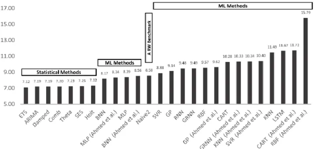
Figure 19 – Forecasting performance (sMAPE) of the ML and statistical methods included in the study (Makridakis et al. 2018, 15) ... 45

Figure 20 – Forecasting performance (sMAPE) versus computational complexity (Makridakis et al. 2018, 18) ... 46

Figure 21 – Preprocessing phases ... 64

Figure 22 – A depiction of X and Y ... 65

Figure 23 – A depiction of X and Y examples... 66

Figure 24 – Combined interpolation and reshaping function... 66

Figure 25 – The train-test split ... 67

Figure 26 – Recurrent GRU or LSTM neural network architecture ... 69

Figure 27 – The architectures and the number of parameters ... 71

Figure 31 – The average estimates for the three smallest LSTM and GRU architectures 82

Figure 32 – The third GRU-4 iteration ... 84

Figure 33 – Model capacity and fit ... 85

Figure 34 – Test set MSE over the training epochs the three largest LSTM and GRU architectures ... 86

Figure 35 – The average estimates for the three largest LSTM and GRU architectures 88 Figure 36 – The average estimates for three midsize LSTM and GRU architectures .... 90

Figure 37 – LSTM-32-16 predictions ... 92

LIST OF TABLES Table 1 – U.S. recessions between 1980 and 2015 (NBER, 2019b)... 11

Table 2 – Abbreviations for the data tables ... 57

Table 3 – Economic variables ... 57

Table 4 – Financial variables ... 60

Table 5 – Behavioral variables ... 62

Table 6 – The selected recurrent neural network architectures ... 70

Table 7 – Architectures and epochs ... 74

Table 8 – Architectures and MSE for ensembles ... 78

Table 9 – Architectures and MAE for ensembles ... 78

policies. However, predicting these fluctuations, especially the timing of recessions, has been proven to be a difficult task (Rudebusch & Williams 2008, 2; Zarnowitz & Braun 1992, 21), making it an interesting area to try to develop more accurate methods.

According to universal approximation theorem by Hornik et al. (1989, 363-364), a feedforward network with at least one hidden layer and nonlinear activation functions, can theoretically represent any function, linear or nonlinear. This unprecedented ability to represent functions that have been difficult with other current methods has made arti-ficial neural networks (ANNs) stand out in problems that demand a very high modeling capacity from the applied model. However, finding a suitable ANN and optimizing its parameters has been found challenging, but lately, together with more enhanced methods, suitable data and computational resources, applying these methods has become more con-venient. (Géron 2017, 258; Goodfellow et al. 2016, 280-290.)

Because of these advances related to finding suitable ANNs and optimizing them, together with a large amount of existing economic data, these methods can be recognized as noteworthy tools for economists and especially for making predictions (Varian 2014, 1, 6, 20-21). The predictions and insights that are made by using these sophisticated ma-chine learning methods can be particularly helpful for policymakers in new ways that were not common, or even possible, with standard econometric methods (Basuchoudhary et al. 2017, 1). However, using ANNs in the domain of economics is relatively new, but interesting, because of the linear models’ incapability to model many real-world pro-cesses that appear to include nonlinearity (Binner et al. 2004, 2).

This study compares different size recurrent neural networks (RNNs) in predicting business cycles for the U.S. The proposed RNNs consist of either long short-term memory cells (LSTMs) or gated recurrent units (GRUs) and they are trained with multivariate data that comprises 27 time-series of several economic, financial and behavioral indicators. The RNNs are configured so that, per example, each model used 26 explanatory varia-bles’ observations for the previous 400 days to generate a 91-day forecast of the U.S. business cycle. The results for the comparison are done by using a train-test split, where the models are trained with data from the time period between 1980 and 2005, and eval-uated by using the data from the following ten years. Each proposed RNN architecture is

trained three times to counter the randomness and stochasticity that the training algorithm introduces to the parameter optimization process.

The research is conducted so that it answers the following three research questions. Firstly, does the proposed methods suit predicting business cycles. Secondly, how large RNN architecture appears suitable for the task at hand. Thirdly, which method, LSTM or GRU, suits better the prediction problem.

This study examines methods that are relatively little studied in the domain of eco-nomics and, simultaneously, they appear to offer a vast number of potential applications. For this reason, this study tries to offer a reference point for the following studies and, hence, it concentrates on applying only common and approved methods. The main focus is on examining the performance-related effects of using different RNN models. The eval-uation is done by using typical performance metrics, such as mean squared error (MSE) and mean absolute error (MAE). However, to gain a deeper understanding, the plots of the predictions for the testing set are examined. Appropriate early warning signals are considered beneficial, but evaluating them is recognized somewhat subjective. Thus, the evaluation favors more objective indicators.

The research is organized into five separate sections. The theoretical background is split into two separate chapters. The first chapter concentrates on presenting the necessary theoretical foundations related to the business cycles, time-series analysis and the chosen methods. The theory review should offer the necessary knowledge for understanding the results and the motivations behind the chosen methods. Therefore, in order to serve com-mon economics practitioners, the selected deep learning (DL) methods are introduced carefully. The second chapter introduces the related literature that comprises the previous studies related to time-series analysis, finance and economics. The previous studies indi-cate the proposed methods’ weaknesses and strengths, along with suggesting suitable ap-plications. The literature review also presents a timeline that helps to connect this study to the existing work and further motivates using these novel RNN methods for complex macroeconomic prediction problems. After the related theory and literature are reviewed, the chosen methods are examined in more detail in the fourth chapter. This chapter covers the data examination, the selected preprocessing methods for the data, the training algo-rithm and the proposed RNN architectures that are used for generating the results. The results are examined in the fifth chapter, that is followed by the conclusions.

time-series can be defined as

𝑥1,𝑇 = {𝑥𝑡|𝑡 = 1, … , 𝑇},

where 𝑥_1,𝑇 is a time-series for a time interval [1, 𝑇], 𝑥_𝑡 is either a scalar or a vector that includes the realizations for time step 𝑡 and 𝑇represents the number of captured realiza-tions. If the realizations 𝑥_𝑡 for the time interval are scalars, the time-series is one-dimen-sional, but if they are vectors, the time-series is two-dimensional and can be denoted as a matrix 𝑋1,𝑇. Continuous processes can be tracked by collecting records of the process over time, creating a discrete time-signal. In time-series analysis, the examined processes are often stochastic, meaning that these collected realizations 𝑥𝑡 are generated by some random process that draws these values from some set of all the possible values according to some distribution function. (Lütkepohl 2005, 1-4.)

According to Längkvist et al. (2014, 3-4), time-series data has several unique prop-erties that distinguishes it from other types of data. The following description of these properties follows the structure and content that they used in their study.

Firstly, time-series data usually contains noise that can make it harder to find valuable information from the data. For example, in the area of economics, the daily movements are not usually important when trying to extract information about the macro trends that occur more slowly and are not affected significantly by small frequent short-term move-ment.

Secondly, the underlying process might be very complex and, therefore, understand-ing and modelunderstand-ing it tolerably, even by analyzunderstand-ing all the available time-series data, might still be too challenging or even impossible with the best possible techniques available.

Thirdly, time-series data can have the same value at different time steps, meaning either the same or something else depending on, for example, some previous values. Mod-eling this time-dependency correctly is challenging for many reasons, but also because the length of a sequence for capturing this relationship could be unknown. This, in turn, could make the selection of a suitable model and the related methods difficult.

Lastly, there is stationarity. Since a realization 𝑥_𝑡 can be captured only once at any given time unit 𝑡, it is not possible to identify the mean or variance of all the possible

realizations of 𝑥_𝑡 per time unit 𝑡. For example, it is impossible to observe two or more different realizations of the S&P 500 index at any given time unit. However, the mean and covariance can be calculated for some time-series 𝑥_1,𝑇 by using the realizations over some time interval [1, 𝑇]. For example, in order to use several popular autoregressive models and their extensions, the time-series data should be weakly or strongly stationary. A time-series is weakly stationary if

𝐸(𝑥𝑡) = 𝜇 and 𝐶𝑜𝑣(𝑥𝑡, 𝑥𝑡+ℎ) = 𝛾𝑡,𝑡+ℎ= 𝛾ℎ,

meaning that the expected value 𝜇 for a realization 𝑥_𝑡 is a constant, and the covariance between values 𝑥𝑡 and 𝑥𝑡+ℎ depends only on their distance between each other, denoted here as ℎ. Strong stationarity is achieved when series values’ distribution is time-invariant. For example, time-series 𝑥_1,𝑇 is strictly stationary if the joint distribution func-tion is identical for any two different subsets of 𝑥_1,𝑇 that share the same length, such as, 𝑥_1,5 and 𝑥_10,15. (Hamilton 1994, 45-46; Tsay & Chen 2019, 2.)

Time-series analysis is a method for extracting knowledge from time-series data. By performing a time-series analysis, one can better understand the past, but also, use the extracted information to make predictions about the future. (Nielsen 2019, 1.) To make predicting plausible, data from important variables should be available, and it should con-tain useful information related to the future developments of the chosen variable or vari-ables. With this data, some function 𝑓(∙) can be found that could be used to make predic-tions for one time step 𝑡 + 1 or several time steps [𝑡 + 1, 𝑡 + ℎ] ahead. The latter type of method is called sequence-to-sequence predicting, and it can be demonstrated for variable 𝑦 by using multivariate data 𝑋 as follows

𝑦̂_{𝑡+1,𝑡+ℎ}= 𝑓(𝑋_{𝑡−𝑘,𝑡}, 𝜃),

where 𝑦̂_{𝑡+1,𝑡+ℎ} denotes a sequence of predictions for an interval [𝑡 + 1, 𝑡 + ℎ], 𝑋_{𝑡−𝑘,𝑡} the input matrix containing several variables’ sequential data for time steps [𝑡 − 𝑘, 𝑡] and 𝜃 the function 𝑓 parameter values. (Lütkepohl 2005, 1.)

Various different models can be used for modeling the relationships between 𝑋𝑡−𝑘,𝑡 and 𝑦̂_{𝑡+1,𝑡+ℎ}, but some of them suit the problem better than the others. Finding a suitable model can be recognized as a model selection problem and, thus, it is related to the area of machine learning (ML). This study applies the typical ML approaches for finding a suitable model for the task at hand, that is modeling the relationships between the past values of the chosen 26 indicators and the future values of the U.S. business cycle.

occasional in their nature. Each cycle includes one upward and downward motion, also called respectively as expansion and recession. Various definitions exist for these con-cepts and, therefore, different actors might have different views on the economic situation of different economies. For the U.S., the National Bureau of Economic Research’s Busi-ness Cycle Dating Committee determines the dates when its economy has a recession or expansion. According to NBER (2019), this decision is made by analyzing economic ac-tivity in the U.S. broadly and

“A recession is a period between a peak and a trough, and an expansion is a period between a trough and a peak.”

The historical record of the recessions in the U.S. can be found from NBER’s website1_, but also from the Federal Reserve Economic Data (FRED) databank2_{. This study} com-prises the time period between 1980 and 2015. During that time, the U.S. has experienced five recessions, shown in table 1.

Table 1 – U.S. recessions between 1980 and 2015 (NBER, 2019b)

Peak Trough Length (months)

January 1980 July 1980 6

July 1981 November 1982 16

July 1990 March 1991 8

March 2001 November 2001 8

December 2007 June 2009 18

Between the years 1980 and 2015, the U.S. has spent most of the time in economic ex-pansion. The economy has spent a total of 56 months in recession and 364 months in expansion. Recessions’ share of the time period is approximately 13.334%, making them significantly rarer than the expansions, but not rare enough to be recognized as outliers. Though their scarcity makes the process of learning to predict them difficult, there are no appropriate methods to overcome these disbenefits.

1 _{http://www.nber.org/cycles/cyclesmain.html} 2 _{https://fred.stlouisfed.org/series/USREC}

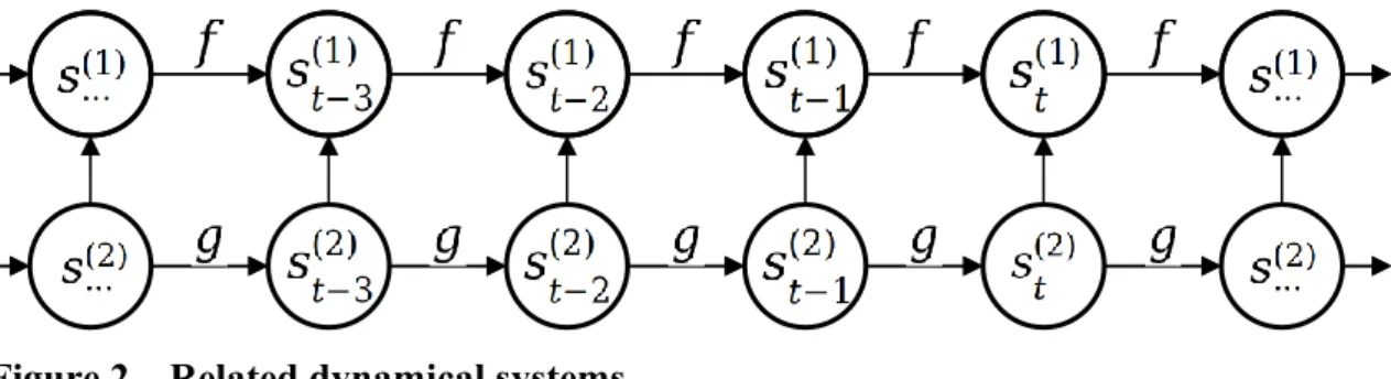
2.3 Business cycles as a dynamical system

In economics, a sequence is a subset of real numbers for some time interval 𝐼 (Giordano et al. 2013, 7). In this domain, the interval under consideration is typically limited to

𝐼 = [0, +∞),

(Barnett et al. 2015, 1751), where 0 denotes the first realization available. A dynamical system is a process that generates realizations over time that can be stored in a sequence to form a time-series. By using the known realizations, it is possible to describe the change from one time step to the next by estimating some function 𝑓 (Giordano et al. 2013, 5-7).

The economy can be seen as a dynamical system that evolves in time, generating realizations whose fluctuations can be defined as business cycles. The classical dynamical system can be described as follows

𝑠_𝑡(1) = 𝑓(𝑠_𝑡−1(1), 𝜃(1)),

where 𝑠_𝑡(1) resembles the state of the system at discrete time step 𝑡, and it is defined by some function 𝑓, previous state 𝑠_𝑡−1(1) and some set of parameters 𝜃(1)_{. One important} as-pect of this process is that it is recurrent, meaning that the state 𝑠_𝑡(1) is dependent on its previous states, as depicted in figure 1. (Goodfellow et al. 2016, 369.) In addition, the formula can be decomposed to show the recurrence:

𝑠_𝑡(1) = 𝑓(𝑓(𝑓(𝑠_𝑡−3(1), 𝜃(1)), 𝜃(1)), 𝜃(1)).

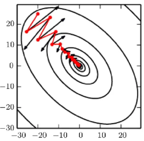
Figure 1 – Dynamical system

This type of dynamical system’s change over time can also be affected by some external dynamical system 𝑠_𝑡(2), that is unique, but has similar properties to the first dynamical system 𝑠_𝑡(1). The function for the first dynamical system can be now written as

𝑠_𝑡(1)= 𝑓(𝑠_𝑡−1(1), 𝑠_𝑡(2), 𝜃(1)),

where the first dynamical system’s state at time step 𝑡 depends on its previous state 𝑠_𝑡−1(1), some external system’s current state 𝑠_𝑡(2) and some set of parameters 𝜃(1)_{, as depicted in} figure 2. In this type of situation, one should also understand what is the second dynamical system’s effect on the first dynamical system.

Figure 2 – Related dynamical systems

As mentioned earlier, these types of systems can be tracked by collecting realizations over time. The resulting time-series allow creating models that try to replicate the rules that define how the dynamical system evolves in time. As mentioned previously, the economy can be recognized as a dynamical process that affects and is affected by several different other dynamical systems. Because of these attributes, it is justified to use multi-variate data that includes some set of so-called leading indicators, that comprises infor-mation of several dynamical systems, for predicting business cycles (Qi 2001, 383-384). 2.4 Supervised machine learning

Machine learning (ML) is defined by Samuel (1959, 1) as a way to program a digital computer so it can be thought to be able to learn, or by Goodfellow et al. (2016, 96) as a study of designing algorithms that can learn from data.

ML has a close relationship with other common data analyzing and modeling tools since they share several methods and tools. According to Varian (2014, 5-6), in statistics and econometrics, the data analysis can be broken into four categories: 1) prediction, 2) summarization, 3) estimation and 4) hypothesis testing. He suggests that the major dif-ference between ML, common statistics and econometrics is that where statisticians and econometricians focus primarily on insights and relationships that can be found from the data, ML concentrates mostly on making accurate predictions. Thus, ML should be con-sidered when the focus is on predicting.

Machine learning can be divided into two main classes, that are a predictive and de-scriptive approach (Murphy 2012, 2). The predictive ML algorithms can be used for pre-dicting some missing information by using some known information, and the descriptive ML algorithms are typically used for finding and describing patterns in data. The algo-rithms for the predictive tasks are commonly trained by using supervised learning meth-ods and the latter by using unsupervised learning methmeth-ods. It is also good to acknowledge that there are many other ways to classify different types of machine learning, but they

are out of the scope of this study, which only applies supervised learning algorithms for business cycle forecasting.

In supervised learning, algorithms are provided with input-output pairs. (Hastie et al. 2009, 29; Goodfellow et al. 2016, 103.) Inputs can be defined, for example, as a matrix 𝑋 ∈ ℝ𝑖×𝑗 where 𝑖 represents the number of examples or rows in the data and 𝑗 represents the number of explanatory variables or features. In turn, similarly to the inputs, also the outputs can be defined by using some common data object, such as a matrix 𝑌 ∈ ℝ𝑖×𝑘 _or a vector 𝑦 ∈ ℝ𝑖𝑥1_{, depending on the number of dependent variables 𝑘.}

A supervised machine learning prediction problem can be described with the follow-ing equation:

𝑓(𝑥(𝑖), 𝜃) = 𝑦̂(𝑖)_.

Here the vector 𝑥(𝑖) _{represents the 𝑖}th _{example, that is on row 𝑖 in the data matrix 𝑋. 𝑓(∙)} represents some function, 𝜃 the function’s parameters and 𝑦̂(𝑖) the outputs for the 𝑖th in-puts. In supervised ML, the task is typically to find some function with some set of pa-rameters that is able to achieve satisfying accuracy at mapping the known input values into estimated output values that are as close as possible to the real output values. (Varian 2014, 6; Goodfellow et al. 2016, 103-105.)

In machine learning, it is recognized that there are plenty of different types of models that suit different types of tasks and data. Therefore, much of the ML theories and meth-ods concern finding a suitable model for a given problem and data. For example, classi-fication, regression and clustering tasks have their own typical models and other data related techniques, but behind it all, there lies a fundamental theory that motivates ques-tioning the current common practices and testing new methods. According to Wolpert (1996) and Wolpert and Macready (1997) papers’ mathematical demonstrations, if abso-lutely no assumption about the data or the task is made, no model or algorithm is better than all the other possible alternatives in every different task. Therefore, in this situation, one should evaluate all the possible options, also called the hypothesis space, in order to find the solution that fits the given problem the best. These theorems are called the No Free Lunch theorems (NFL-theorems), and they are recognized as one of the most im-portant theories in the field of ML.

However, Géron (2017, 31) notes that, in practice, evaluating all the different possi-ble models is impractical, or even impossipossi-ble with the scarce resources and, hence, some assumptions about the data and the task should be made in order to narrow down the set

2.5 Bias-variance trade-off

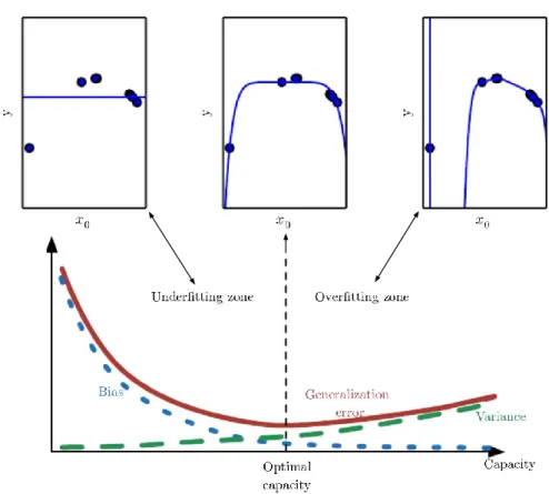
Bias, variance and their trade-off are fundamental at understanding the essential concepts of machine learning, such as under- and overfitting, generalization error and model ca-pacity, which build the framework for finding a suitable model for some prediction task. Typically, error in an estimator can be divided into two components: bias and variance. Bias addresses the amount of error that occurs from the prediction’s expected deviation from the real value, and variance tells how much error is generated from the deviation of the expected prediction from the real prediction. (Goodfellow et al. 2016, 120-128; Ge-man et al. 1992, 2.)

In this study, the mean squared error (MSE) is the most important error measure because it is used in parameter optimization and model evaluation. By following Mur-phy’s (2012, 202) notations, we can derive the expected bias and variance for the expected MSE as follows 𝑀𝑆𝐸 = 𝔼[(𝑦̂ − 𝑦∗)2], 𝑀𝑆𝐸 = 𝔼 [((𝑦̂ − 𝑦̅) + (𝑦̅ − 𝑦∗))2], 𝑀𝑆𝐸 = 𝔼[(𝑦̂ − 𝑦̅)2_{] + 2(𝑦̅ − 𝑦}∗_{)𝔼[𝑦̂ − 𝑦̅] + (𝑦̅ − 𝑦}∗₎2_], 𝑀𝑆𝐸 = 𝔼[(𝑦̂ − 𝑦̅)2] + (𝑦̅ − 𝑦∗₎2_, 𝑀𝑆𝐸 = 𝑣𝑎𝑟(𝑦̂) + 𝑏𝑖𝑎𝑠2(𝑦̂), 𝑀𝑆𝐸 = 𝑣𝑎𝑟𝑖𝑎𝑛𝑐𝑒 + 𝑏𝑖𝑎𝑠2.

Here, 𝑦̂ stands for the prediction, 𝑦∗ _{for the real value, and 𝑦̅ for the expected prediction} for a given input. The expected MSE and the expected prediction 𝑦̅ can be discovered by testing the model repeatedly by using a large number of training data and then averaging the result (James et al. 2013, 34).

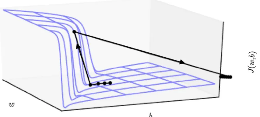
From the decomposition, one can see that, in order to minimize MSE, both variance and bias should be decreased. However, they are connected to model capacity, as depicted in figure 3.

Figure 3 – The bias-variance trade-off (Goodfellow et al. 2016, 118, 128)

Generally, the models with too low modeling capacity for modeling some data tend to have high bias and low variance, and in turn, the models that possess too much modeling capacity tend to have small bias but high variance. This happens because the more capable models are able to model the random noise in the data and become too sensitive to small changes in the input data and, thus, gain more variance when tested with unseen data. This phenomenon is also called overfitting. In turn, underfitting occurs when using insuf-ficient models that are too constrained to find a suitable fit for the data. These two phe-nomena are interlinked by the modeling capacity, and they form a theory called the bias-variance trade-off. (Goodfellow et al. 2016, 127-128; James et al. 2013, 33-36.)

An estimate of a model’s true performance, also called the generalization error, can be obtained by testing the model with examples that are not used for tuning its parameters. This estimation is usually done by dividing the available data into two or more folds that are then used either to train or to test the model. (Goodfellow et al. 2016, 108-111.) In this study, the generalization error is estimated by dividing the whole data into two folds where one is used for model training and the other for estimating the generalization error. The methods used in this study for dividing the data into training and testing sets are examined in more detail in section 2.6.4.

In fact, finding good quality data and preprocessing it accordingly is found as one of the most important areas in ML. (Nielsen 2019, 17; Géron 2017, 26.)

In this study, the motivation for the chosen preprocessing methods comes from three sources. Firstly, deep learning solutions prefer particular types of properties from the data. Secondly, time-series data has its own ways when it comes to preprocessing. Thirdly, the preprocessing should be done in a way that is also possible in the production environment. Essentially, this means that the preprocessing methods should not use information from the time steps that are not known at some particular moment for some particular instance. In this study, for convenience, only the future information is cropped when preprocessing. It does not take into account the lag between the date when a realization occurs and the date when it is actually released.

The time-series data used in this study had several imperfections, such as missing values, incoherent value scales and trends. These defects have been handled by using common preprocessing methods that are introduced in the following sections.

2.6.1 Linear interpolation

The data used in this study suffers from missing values that mostly originate from low-frequency time-series. In order to obtain more data for the data-hungry deep learning methods, daily data is used. Hence, all the time-series with a lower frequency demand upsampling.

Interpolation is a common method for handling missing values and upsampling. It approximates missing values in a time-series by using their neighboring data points. In this study, a linear interpolation is used, whose equation is

𝑦(𝑡)= 𝑦(𝑡−1)+

(𝑥(𝑡)−𝑥(𝑡−1))(𝑦(𝑡+1)−𝑦(𝑡−1)) 𝑥(𝑡+1)−𝑥(𝑡−1) ,

where (𝑥_(𝑡−1), 𝑦_(𝑡−1)) and (𝑥_(𝑡+1), 𝑦_(𝑡+1)) are the known data points that are used for finding the missing coordinate 𝑥_(𝑡) or 𝑦_(𝑡). Linear interpolation can also be used to fill a chain of missing values, for example, when upsampling quarterly data into daily data. Figuratively, it draws a line between two known realizations and the missing values in that range are filled by using this particular line, as depicted in figure 4.

Figure 4 – A depiction of linear interpolation

If there are no realizations before or after the missing value, the adjacent slope can be used. In this study, the previous slope is used for the last missing values that would not otherwise receive a value. As depicted in figure 4, the missing value for time step 𝑡 + 2 would be set by using the slope determined by the realizations for time steps 𝑡 − 1 and 𝑡 + 1. In turn, when dealing with the first missing values, this same slope could be used. However, in this study, the previous realizations are used for determining these missing values in order to get more accurate time-series. Thus, for example, the realizations for time steps 𝑡 − 3 and 𝑡 − 1 are used for determining the value for the missing realization on time step 𝑡 − 2. Here, the 𝑡 − 3 realization is drawn from outside of the data sequence under consideration, an area called interpolation buffer. This method should not be used for the last missing values if one wants to simulate a situation where there is no infor-mation about future values and prevent the aforementioned lookahead effect.

Linear interpolation has some defects. Firstly, the realizations of a dynamical system seldom follow the aforementioned equation. Hence, a time-series that is impaired of miss-ing values cannot be fully repaired by usmiss-ing linear interpolation and, therefore, time-series with fewer missing values should be preferred. Secondly, the adjacent data points’ ability to provide valuable information about the missing value or many values between them might be weak, for example, when the signal is very similar to a random walk or is oth-erwise very volatile. Thirdly, if used incorrectly, it might also provide lookahead infor-mation to the data. (Nielsen 2019, 48-50.)

Even though of these defects, interpolation is a useful method for handling the miss-ing values since it enables the use of some valuable time-series. Moreover, the trends in macroeconomic data tend to be medium and long-term movements, making the short-term variations less significant and, therefore, allowing more short-short-term imprecision from

A trend in the context of time-series data is typically a systematic change that is not sea-sonal. A trend in a time-series can be detected, for example, by examining its plot or by testing its stationarity. In economic time-series, trends are typical because several eco-nomic processes’ realizations depend on their previous values. Zhang and Qi (2002; 2005) showed that if a time-series contains trends and seasonal variations, both should be pre-processed before feeding it to an ANN model. Furthermore, Qi and Zhang (2008) demon-strated that differencing should be used for detrending a time-series.

Because ANN models can deal with nonstationary data, stationarity tests are not im-plemented in this study, and differencing is used for handling only the time-series with notable trends that can be detected by exploring their plots. The differencing is done by using the previous time step value. No deseasonalization is implemented to the time-se-ries, but several already deseasonalized time-series are used.

2.6.3 Min-max scaling

When using deep learning, the data is typically scaled between 0 and 1 (Bengio 2012, 447). Because many scaling or normalization methods use minimum and maximum val-ues, they are vulnerable to trends and outliers. If a trend continues after the parameters for the scaling function are set, it is likely that the future data can cross the boundaries if the scaling parameters are not adjusted. The notable trends are handled in this study and, therefore, the common min-max scaling equation:

𝑥𝑠𝑐𝑎𝑙𝑒𝑑 = (𝑥 − 𝑥𝑚𝑖𝑛)/(𝑥𝑚𝑎𝑥 − 𝑥𝑚𝑖𝑛),

should be feasible for scaling the time-series data. In min-max scaling, some value from a time-series 𝑥, or the whole time-series, is scaled by using its the smallest 𝑥_𝑚𝑖𝑛 and highest 𝑥_𝑚𝑎𝑥 value. Each time-series is scaled separately.

Although this method is popular, it is vulnerable to outliers because it utilizes the minimum and maximum values. The data used in this study is relatively smooth, and it does not seem to include significant changes that could not be explained. Moreover, for this particular application, some rare values typically have a reasonable explanation and, therefore, might be necessary when predicting business cycles.

2.6.4 Train-test split

To estimate the generalization error of some model, which is the expected value of some chosen error measure, such as MSE, when averaged over the future data, one can use a common method called a train-test split. It is applied by dividing a data set once into two separate sets: the training set, that is used for optimizing the models’ parameters, and the testing set, that, in turn, is used for testing the models’ performance with unseen data examples, hence yielding an estimate of the models’ generalization error. (Goodfellow et al. 2016, 108-111; Murphy 2012, 23.) One crucial aspect of this method is to define the training and testing sets in a way that simultaneously maximizes the models’ performance and the accuracy of the generalization error estimate. Furthermore, when defining the split, a trade-off should be acknowledged. Since, generally, the more data is used for op-timizing the model, the better the model performs, and in turn, the more data is used for evaluating the model, the better estimate of the generalization error is achieved. Hence, when using train-test split, it tends to give pessimistic estimates of the generalization er-ror, compared to what the models could achieve by using the whole available data. More-over, the sets should be somewhat similar to each other. The training set should contain the information, the so-called general pattern, to be learned, and the testing set should test how well the models learned to model this pattern and, hence, it needs to contain a suffi-cient number of examples about the general pattern. (Goodfellow et al. 2016, 108-111.)

When dealing with time-series data, both, the training and testing set, should contain a continuous sequence of consecutive examples that form a continuous time window. Furthermore, when trying to predict the future by using past information, the sequence used for testing should contain the newer data points, and the training set the older data points, in order to simulate the real-life use case. (Nielsen 2019, 343.)

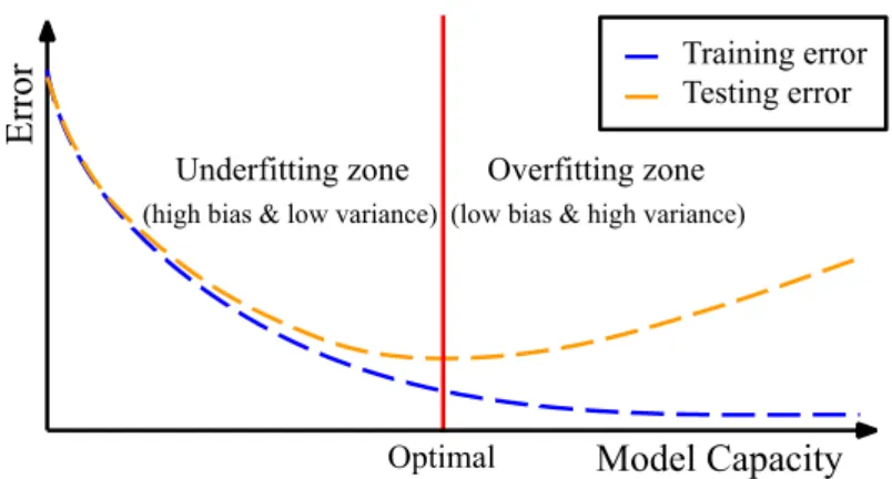
As introduced in the NFL-theorems, there is no universally superior model for every possible prediction problem. Instead, any model from the vast hypothesis space should be considered as a possible option if no assumptions are made concerning the task at hand. A model suitable is commonly found based on the bias-variance trade-off framework, together with some performance measures that guide the decisions concerning the model capacity. Generally, a complex problem demands a model that is able to model complex relationships and vice versa (Goodfellow et al. 2016, 112-113).

generalization error. Hence, when the model underfits or overfits the data, the testing error should increase due to the bias-variance trade-off. A model with less than the optimal modeling capacity has trouble to capture the general pattern adequately. Though these models cannot offer the best performance, they might be useful for providing information about the task at hand, possibly about the most important relationships. When the model capacity is increased over the optimal value, the model can adjust itself better to the train-ing set specific noise and other irregularities that weakens its ability to perform well with unseen examples in the training set. (Goodfellow et al. 2016, 108-114, 127-128; James et al. 2013, 33-36.)

Figure 5 – A depiction of a typical relationship between model capacity, training error and testing error

The train-test split is done in this study by dividing the data into two separate time win-dows where the latest data is used for testing and the rest for training a selection of artifi-cial neural network models. In order to make the testing set adequate, it should include the general pattern, here the business cycle. Hence, the whole time-series data is divided so that the testing set includes the latest U.S. business cycle between 2005 and 2015. The chosen train-test split together with all the selected time-series are introduced in more detail in sections 4.1. and 4.2.3.

2.7 Deep learning

An artificial neural network (ANN) with more than one layer between the input and out-put layers is considered deep. These types of ANNs are called deep neural networks (DNNs) and all the methods concerning finding a suitable DNN and its parameter values more broadly as deep learning (DL) (Goodfellow et al. 2016, 8-18). Hornik et al. (1989) proved that a classical ANN model, a multilayer perceptron (MLP) that possesses a suf-ficient number of units with nonlinear activations function can approximate any continu-ous function at an arbitrary level of accuracy. For this reason, ANNs are regarded as uni-versal function approximators. Since their very high capacity to model complicated pat-terns in data, DL algorithms have enjoyed success in extremely complex domains, such as, image and speech recognition that were not conquered by any other models. (Good-fellow et al. 2016, 152, 225.)

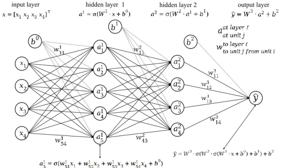
In deep learning, the model consists of numerous individual arithmetic operations that together form a bigger entity, a network of small functions that is optimized, for example, to map inputs to outputs if the task is a supervised learning problem. Before introducing the more advanced ANNs that are used in this study, a multilayer perceptron (MLP) is explained, which serves as a background. A common way to examine ANNs is by studying their architecture from a computational graph or some other depiction. In this way, the computations might be easier to be perceived and the network’s main traits to be evaluated (Goodfellow et al. 2016, 201).

weights. For example, an activation for unit 𝑎₅1 _{is calculated by taking a weighted sum of} the previous layer’s activations and their relative weights for the examined unit that is then added to the bias term 𝑏0_{, following some activation function to introduce} nonline-arity. Several different functions can be used as an activation function, such as sigmoid 𝜎 or hyperbolic tangent 𝜏. The activation 𝑎₅1 can now be written in a vector notation by using dot product as follows

𝑎₅1 = 𝜎((𝑤₅1)⊤𝑥 + 𝑏0).

As depicted in figure 6, the activations for layer 𝐿 are calculated with the previous acti-vations 𝑎𝐿−1 _{or inputs 𝑥, the matrix 𝑊}𝐿 _{that consists of the relative transposed weight} vectors 𝑤_𝑗𝐿 _{for each separate unit 𝑗 in the layer 𝐿, the bias term 𝑏}𝐿−1 _{and some activation} function as follows

𝑎𝐿 _{= 𝜎(𝑊}𝐿_𝑎𝐿−1_{+ 𝑏}𝐿−1_).

The examined MLP in figure 6 consists of one input layer, two hidden layers and one output layer. These layer operations formulate a chain of functions that yields the output 𝑦̂ in the following way

𝑓(𝑥, 𝜃) = 𝑊3_𝜎(𝑊2_𝜎(𝑊1_{𝑥 + 𝑏}0_{) + 𝑏}1_{) + 𝑏}2 _{= 𝑦̂,}

where 𝜃 consists of all the parameters in the model, which are the weights 𝑊𝐿 and the bias terms 𝑏𝐿_{. In this example, the output layer does not apply an activation function.} (Goodfellow et al. 2016, 164-172; Graves 2012, 12-16.)

To control the model capacity in DL, one has to adjust the architecture and possible regularization terms. Generally, the more a model has parameters and less regulation, the higher is its ability to model complex patterns and the more prone it is to overfit to the provided data. The depth of the examined MLP model is three. Essentially, all layers other than the input layer are counted. The width of a layer is determined by the number of units it has. Several studies have found that typically larger architectures tend to be the most successful if they are regularized properly, especially the networks with higher depth. (Bengio 2012, 450-451; Goodfellow et al. 2016, 165, 193-197.) Although the uni-versal approximation theorem shows that an ANN with just one hidden layer and a suffi-cient number of units can represent any continuous function, deeper models are favored.

Typically, depth gives more modeling capacity with fewer parameters and, thus, requires less computational resources, albeit exposing the training process to more faults, such as exploding and vanishing gradients. (Goodfellow et al. 2016, 193-197, 285-287.)

This MLP model is also classified as a deep feedforward network that comes from the nature of how the activations are propagated through the network, which is forward layer-by-layer. In addition to forward propagating networks, there are also networks with connections that allow them to feed activations back into the network, called recurrent neural networks. (Goodfellow et al. 2016, 164.)

2.7.1 Recurrent neural networks

Recurrent neural networks (RNNs) are a class of ANN models that include recurrent con-nections in their architecture. Feeding information back into the network builds a memory-like function to RNN models, which makes them more suitable for some sequen-tial tasks than the typical feedforward networks. (Goodfellow et al. 2016, 367; Graves 2012, 18-19.)

Figure 7 – A depiction of a classical recurrent unit

Similarly to the normal hidden units that were introduced in the MLP example, a recurrent unit 𝑎₁ receives a bias term 𝑏 and inputs 𝑥 at time step 𝑡 that are multiplied with their relative weights, as depicted in figure 7. The addition is the recurrent connection that multiplies some activation at the previous time step, that is here its own previous activa-tion 𝑎1,(𝑡−1) with its relative weight 𝑣11. After these arithmetic operations, an activation function 𝜎 is introduced to add nonlinearity to the recurrent unit’s activation. (Goodfellow et al. 2016, 369-376; Graves 2012, 18-21.) The function for this classical recurrent unit at time step 𝑡 can be written by using a vector notation as follows

𝑎_1,(𝑡) = 𝜎(𝑤⊤_𝑥

Figure 8 – A depiction of a recurrent neural network

An RNN with one hidden layer comprises three weight matrices 𝑊₂₁, 𝑊22 and 𝑊32, as depicted in figure 8. The bias terms can be regarded as input nodes that feed forward a value of one that is multiplied by a weight parameter and, thus, can be included in the weight matrices to simplify the notations. During a forward pass, the RNN generates a prediction 𝑦̂ for time step 𝑡 according to the following equation:

𝑦̂(𝑡) = 𝑊32𝜎(𝑊21𝑥(𝑡)+ 𝑊22𝑎(𝑡−1)1 ),

which resembles the MLP model apart from the recurrent connections 𝑊₂₂𝑎_(𝑡−1)1 . To illustrate how an RNN operates with sequential data, the computational graph can be unfolded with respect to time steps so that the recurrence stands out better, as depicted in figure 9. The model is given the sequential input data one time step at a time, and with every input, the model is able to produce an output for that particular time step.

Figure 9 – An unfolded computational graph

RNNs are able to use past information to make predictions, but RNNs that consist of only the classical recurrent units perform poorly when modeling long-term dependencies in sequential data (Bengio et al. 1994). This is due to the common problems in deep learning,

called vanishing and exploding gradients that might occur when backpropagating the cost to the model parameters (Goodfellow et al. 2016, 390). This defect makes it oftentimes unideal to use this type of RNN for tasks that demand good handling of long-term de-pendencies, and for this reason, the classical recurrent units were introduced only as an introduction to the RNNs and are not used otherwise in this study. Instead, more sophis-ticated methods are chosen that are able to handle better sequences with long-term de-pendencies called long short-term memory cells (LSTMs) and gated recurrent units (GRUs). These gated RNN methods exploit the so-called paths through time that make their training process more robust against the aforementioned issues (Goodfellow et al. 2016, 404). According to the results by Greff et al. (2017) and Jozefowicz et al. (2015) studies, these two aforementioned gated RNN methods seem to perform quite evenly along with few other similar designs in different types of tasks that use sequential data. 2.7.2 Long short-term memory cell

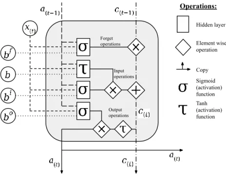
The first version of LSTM was introduced by Hochreiter and Schmidhuber (1997) to cre-ate a method that could overcome the previous RNNs’ problems relcre-ated to modeling long-term dependency. According to Olah (2015), the later versions of the LSTM and its other modifications are widely used in different problems that demand good performance in handling data with long-term dependencies. The following example of an LSTM cell fol-lows the outlines made by Goodfellow et al. (2016, 404-406), Graves (2012, 31-38) and Olah (2015).

An LSTM cell, depicted in figure 10, receives some inputs and produces some out-puts for the next layer and for itself for the next time step, similarly to the previously examined classical recurrent unit. The difference is the architecture of arithmetic opera-tions inside the LSTM cell, along with two different outputs, the activation 𝑎 and the cell state 𝑐. LSTM cell’s core idea is to update the cell state every time step, and then use it to create a cell activation in accordance with some inputs and parameter values. It is this cell state, also called the cell memory, that creates the path through time, and makes the LSTM more robust against the aforementioned unideal backpropagation behavior.

Figure 10 – A long short-term memory cell

The LSTM cell’s arithmetic operations can be seen to construct three gates that control the flow of information in the cell and also out of it. Two of the three gates are dedicated to forget and add information into the cell state as follows

𝑐(𝑡) = 𝑔(𝑡) 𝑓

𝑐(𝑡−1)+ 𝑔(𝑡)𝑖 𝑖(𝑡),

where 𝑐_(𝑡) stands for the cell state at time step 𝑡, 𝑔_(𝑡)𝑓 for the forget gate, 𝑐_(𝑡−1) for the previous cell state at time step 𝑡 − 1, 𝑔_(𝑡)𝑖 _{for the input gate and 𝑖}

(𝑡) for the input, that is now a combination of the previous layer’s current activations, here denoted as 𝑥_(𝑡), and the current layer’s previous activations 𝑎_(𝑡−1). 𝑔_(𝑡)𝑓 , 𝑔_(𝑡)𝑖 _{and 𝑖}

(𝑡) are calculated with op-erations similar to the classical recurrent unit:

𝑔_(𝑡)𝑓 = 𝜎(𝑊𝑓𝑥_(𝑡)+ 𝑉𝑓𝑎_(𝑡−1)+ 𝑏𝑓), 𝑔_(𝑡)𝑖 = 𝜎(𝑊𝑖𝑥_(𝑡)+ 𝑉𝑖𝑎_(𝑡−1)+ 𝑏𝑖),

𝑖(𝑡) = 𝜏(𝑊𝑥(𝑡)+ 𝑉𝑎(𝑡−1)+ 𝑏).

The operation that handles “the forgetting” in the cell is the multiplication between the forget gate 𝑔_(𝑡)𝑓 , that receives a value between 0 and 1 due to the sigmoid activation func-tion 𝜎, and the cell state on the previous time step 𝑐_(𝑡−1). The forget gate should learn when it needs to decrease the cell state and by how much, by finding the right parameter values 𝑊𝑓_{, 𝑉}𝑓 _{and 𝑏}𝑓_{. Similarly, the input gate 𝑔}

(𝑡)𝑖 and the inputs 𝑖(𝑡) should learn when and what they should add to the cell state, by finding the optimal parameters 𝑊𝑖_{, 𝑊, 𝑉}𝑖_, 𝑉, 𝑏𝑖 _{and 𝑏.}

In addition to these operations that concentrate on evolving the cell state, there are operations that determine the actual activation that the LSTM cell outputs at time step 𝑡. These operations are hyperbolic tangent function 𝜏 and the output gate 𝑔_(𝑡)𝑜 _{. The activation} is drawn from the cell state 𝑐_(𝑡) as follows

𝑔_(𝑡)𝑜 = 𝜎(𝑊𝑜_𝑥

(𝑡)+ 𝑉𝑜𝑎(𝑡−1)+ 𝑏𝑜), 𝑎_(𝑡) = 𝑔_(𝑡)𝑜 𝜏(𝑐_(𝑡)).

Similarly to the previous gates, the output gate 𝑔_(𝑡)𝑜 should learn how much it should decrease the mapped cell state at a given time step. However, before applying the output gate, the hyperbolic tangent function maps the cell state between -1 and 1.

An RNN that uses only LSTM cells is called an LSTM network. When compared to the depiction of the RNN in figures 8 and 9, the LSTM cells can be thought to replace the classical recurrent units while maintaining the same layer-wise connections. As can be derived from the LSTM cell’s arithmetic operations, an LSTM network introduces lots of parameters and arithmetic operations. Since computational resources and digital memory are scarce, there has been an incentive to create lighter versions of the traditional LSTM cell, and several modifications have been introduced, one being a gated recurrent unit (GRU).

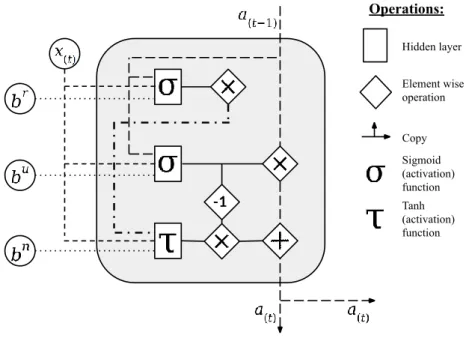
2.7.3 Gated recurrent unit

Cho et al. (2014) created an LSTM variant called a gated recurrent unit (GRU) that re-quires fewer computations but is able to perform similarly in tasks that require modeling long-term dependencies in data. In comparison to an LSTM cell’s architecture, a GRU has only two gates for controlling the information flow inside the unit, whereas an LSTM cell has three. Therefore, it also requires fewer parameters, since it has only three embed-ded hidden layers. Also, a GRU does not have a separate cell state, as shown in figure 11. Instead, it uses the activations from the previous time step 𝑎_(𝑡−1), and the previous layer’s activations at the current time step 𝑥_(𝑡) to produce a new activation 𝑎_(𝑡), according to its arithmetic architecture and parameter values.

Figure 11 – A gated recurrent unit

The activation at time step 𝑡 for a GRU is calculated by the following equation: 𝑎_(𝑡) = 𝑔_(𝑡)𝑢 𝑎_(𝑡−1)+ (1 − 𝑔_(𝑡)𝑢 )𝑎_(𝑡)𝑛 ,

where the new activation 𝑎_(𝑡)𝑛 _{is obtained as follows} 𝑎_(𝑡)𝑛 = 𝜏(𝑊𝑛_𝑥

(𝑡)+ 𝑉𝑛(𝑔(𝑡)𝑟 𝑎(𝑡−1)) + 𝑏𝑛). The functions for the reset and update gate are the following:

𝑔_(𝑡)𝑟 = 𝜎(𝑊𝑟𝑥_(𝑡)+ 𝑉𝑟𝑎_(𝑡−1)+ 𝑏𝑟), 𝑔_(𝑡)𝑢 = 𝜎(𝑊𝑢_𝑥

(𝑡)+ 𝑉𝑢𝑎(𝑡−1)+ 𝑏𝑢).

Similarly to an LSTM cell’s gates, the reset gate 𝑔_(𝑡)𝑟 _{and the update gate 𝑔}

(𝑡)𝑢 should learn when and by how much they decrease the information flow in the unit by discovering suitable values for their weights and biases. The new activation 𝑎_(𝑡)𝑛 _{is obtained by gating} the previous activations 𝑎_(𝑡−1) through the reset gate 𝑔_(𝑡)𝑟 _{and then using the result as an} input alongside with activations from the previous layer, denoted here as 𝑥_(𝑡). Together with the parameters 𝑊𝑛_{, 𝑉}𝑛 _{and 𝑏}𝑛_{, they form an affine function whose output is then} mapped between -1 and 1 by using the hyperbolic tangent 𝜏 as a nonlinear activation function. The activation for the GRU is combined from the previous activation 𝑎_(𝑡−1) and the new activation 𝑎_(𝑡)𝑛 _{in a ratio that is determined by the update gate 𝑔}

(𝑡)𝑢 . (Cho et al. 2014, 3; Goodfellow et al. 2016, 407-408.)

2.7.4 Deep neural network architectures

The more an ANN has learnable parameters, the more it tends to offer modeling capacity, but also its architecture has a significant effect on its ability to express patterns in data. Arguably, the most significant effect comes from multiple hidden layers that are con-nected to each other. (Goodfellow et al. 2016, 165, 193-197.) In theory, the layers closer to the input layer concentrate on finding lower-level details from the data, and the follow-ing layers are able to use these concepts and build higher-level concepts that are relevant for solving the task and decreasing the cost (Goodfellow et al. 2016, 195-197). Although Hornik et al. (1989) have shown that an ANN with only one hidden layer can approximate any continuous function, it is seldom used when applied to complex tasks, because ANNs with more than one hidden layer typically offer better performance with fewer parame-ters. (Delalleau & Bengio 2011; LeCun et al. 2015.)

Several studies, such as Graves et al. (2013), found RNNs with multiple hidden layers offering significant performance gains compared to other established methods at the time. Cho et al. (2014, 3) argue that an LSTM or GRU network with only one hidden layer is able to learn various dependencies over different time scales in the data because of their unique gates. However, Pascanu et al. (2014, 1) suggest that this effect is further strength-ened via additional hidden layers that are able to create higher-level concepts from the previous layers’ activations.

Based on these findings, testing deep recurrent neural networks for the task at hand is reasonable, although they introduce a higher risk for exploding and vanishing gradients. As these risks are acknowledged, the training algorithm for optimizing the selected LSTM and GRU networks includes methods that should make the training process more stable, such as Nesterov accelerated momentum.

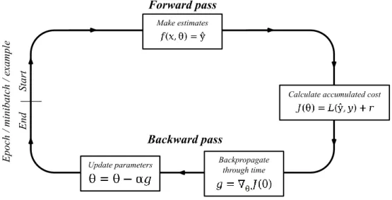
2.7.5 Training epoch

In the context of ML, the parameter optimization is responsible for the phenomenon called learning. Basically, the goal for the parameter optimization in supervised deep learning is to find a set of parameters 𝜃 that minimizes the value determined by some cost function 𝐽(∙). Optimizing an ANN’s parameters is a nonconvex optimization problem since the model itself is nonconvex. Therefore, it does not possess many of the helpful attributes for optimization compared to convex models. Arguably, the most significant difference is that an ANN usually has several local minima. For this reason, it is possible,

(Goodfellow et al. 2016, 149-150, 271-272, 279-285.)

Figure 12 – A training loop

Finding a satisfying set of parameters for an ANN model is usually an iterative process that consists of separate steps, all of which are designed to minimize the cost or provide information about how the optimization process evolves. The steps that are used in this study are depicted in figure 12. During the whole training process, the training set, and typically also the testing set, are fed into the model several times. These datasets can be fed through the training loop all at once, in smaller batches, also commonly called mini-batches, or one example at a time. Typically, only the training set is divided. In the opti-mal scenario, the training set is fed one example at a time. However, it demands lots of computations, especially if the training set consists of a vast number of examples and, hence, minibatches are often used instead. When the whole training set has been fed through the training loop in one way or another, one epoch of training has been carried out. (Bengio 2012, 442-444; Goodfellow et al. 2016, 149-150, 274-276.) This study ap-plies the minibatch training method, and the following sections introduce the steps in the proposed minibatch training loop in more detail.

2.7.6 Forward pass and cost function

The phase where the model receives some inputs and calculates some outputs is called the forward pass and it is generally denoted as

𝑓(𝑥, 𝜃) = 𝑦̂,

where the function 𝑓 is an ANN that transforms some input values 𝑥 into estimates 𝑦̂. These estimates are then used in the next step to determine the cost according to some cost function 𝐽(∙). The cost function typically consists of some loss function and it might also include regularization terms. (Goodfellow et al. 2016, 172, 272.) In this study, mean squared error (MSE) is used for calculating the loss 𝐿(𝑦̂, 𝑦) and an L1 regularization term 𝑙₁ to drive weight decay during the training process. The cost function can be written as follows

𝐽(𝜃) = 𝐿(𝑦̂, 𝑦) + 𝑙₁.

The cost function can be seen to lead the learning process and, hence, it should be examined carefully to better understand the behavior the models learn from the training set. By selecting what type of errors and model attributes generate how much cost, the model can be guided to focus on certain types of patterns in the data, and to produce a certain type of outputs. The following sections provide more details concerning the cho-sen cost function, along with justifying the selected methods.

2.7.6.1 Loss function

Mean squared error (MSE) and mean absolute error (MAE) are both common functions for calculating loss in regression problems. For some minibatch 𝑏, MSE and MAE can be calculated by using equations:

𝑀𝑆𝐸_𝑏 = 1 𝑛∑ (𝑦̂ (𝑖)_{− 𝑦}(𝑖)₎2 𝑛 𝑖=1 , 𝑀𝐴𝐸_𝑏 = 1 𝑛∑ |𝑦̂ (𝑖)_{− 𝑦}(𝑖)_|2 𝑛 𝑖=1 ,

where 𝑛 represents the number of examples in minibatch 𝑏, and 𝑖 the index of an example in the minibatch. When applied in a cost function, the loss function is used for calculating the average loss for a minibatch after example-specific losses have been obtained.

Figure 13 – An error curve comparison between MSE and MAE

In this study, the regression task resembles a binary classification since the business cycle time-series has only two possible values, 1 and 0. However, it is important to acknowledge that the predictions do not exactly represent real probabilities. Because the model treats the task as a pure regression, there are fundamentally no boundaries for the prediction values, but during the training process, the model should learn to target the predictions between 0 and 1. When comparing the equations and the error graphs for the aforementioned interval in figure 13, one can find that MSE generates less or an equal amount of error compared to MAE if the model predicts values between -1 and 1. Whereas MAE can be considered more neutral when it comes to determining how much loss is generated from an inaccurate prediction, MSE would encourage a model to give more significant signals if it finds a risk of a peak or trough happening during the multi-step prediction, since it produces less loss than MAE. This attribute is considered valuable for an application that could be used as an early warning system, although it further averts the predictions from pure probability values. While it is reasonable to penalize less from giving a hint that a peak or trough might occur during the forecasting period, choosing MSE can also be justified by examining the ratio between expansions and recessions. As mentioned in section 2.2, recessions’ share of the whole time period between 1980 and 2015 is only approximately 13.334%. Therefore, it is probable that the model recognizes recessions quite rare and, hence, favors predicting values close to zero. Therefore, in order to encourage a model to output some other values, MSE could be selected over MAE. Furthermore, predicting values over one is unnecessary and, therefore, generating more error for such values is reasonable and should not affect the learning negatively. For these reasons, MSE has been selected as the loss function for the model training process, but both, MSE and MAE, are used for model evaluation in this study.

2.7.6.2 L1 regularization

The L1 regularization consists of one coefficient hyperparameter 𝜆 and the sum of all the parameters’ absolute values:

𝑙1 = 𝜆 ∑𝑃𝑝=0|𝜃𝑝|,

where 𝑃 denotes the number of parameters in the model. Its core idea is to drive parame-ters that model weak, probably unnecessary, relationships or noise close to zero. This method, therefore, helps to reduce the model’s sensitivity to small changes in input values and, hence, decreases the amount of variance the model introduces to its predictions. In addition to the ability to make the training process more robust against overfitting, it can also be seen to further enhance the ANN models’ feature selection properties, where it diminishes the less important relationships’ effect on the output. (Bengio 2012, 451-452.) L1 regularization is used over some other regularization methods because it offers desirable theoretical foundations for more effective feature selection when using noisy multivariate data. Because the multivariate data used in this study contains time-series from several economic indicators, it is probable that some of their own movements alone or their combined representations that are made by the networks themselves are irrelevant when trying to model only the general relationships between the inputs and outputs. In addition to the L1 regularization, there is also a popular L2 regularization method, but according to Bengio (2012, 451), it should not be used together with an early stopping method and, therefore, L1 is preferred instead.

2.7.7 Backpropagation through time

A backpropagation algorithm allows calculating the parameter specific gradients 𝑔, that are then used for updating these parameter values by using some learning algorithm, such as stochastic gradient descent. When using RNNs, the common algorithm for calculating these gradients is a backpropagation through time (BPTT) algorithm. If predictions from multiple time steps are used, not only from the last time step, the loss accumulates from several output values 𝑦̂_𝑡(𝑖) at different time steps 𝑡, as depicted in figure 9. Thus, the ac-cumulated loss for example 𝑖 would be

𝐿(𝑦̂(𝑖), 𝑦(𝑖)_{) = ∑ 𝐿(𝑦̂} 𝑡 (𝑖) , 𝑦_𝑡(𝑖)) 𝑇 𝑡=1 ,

where 𝑇 denotes the number of time steps whose output values are used for calculating the loss. At each time step, the output values are typically calculated by using different