Importance Sampling Schemes for Evidence Approximation in Mixture Models

Importance Sampling Schemes for Evidence

Approximation in Mixture Models

Jeong Eun Lee∗ and Christian P. Robert†

Abstract. The marginal likelihood is a central tool for drawing Bayesian infer-ence about the number of components in mixture models. It is often approximated since the exact form is unavailable. A bias in the approximation may be due to an incomplete exploration by a simulated Markov chain (e.g. a Gibbs sequence) of the collection of posterior modes, a phenomenon also known as lack of la-bel switching, as all possible lala-bel permutations must be simulated by a chain in order to converge and hence overcome the bias. In an importance sampling approach, imposing label switching to the importance function results in an ex-ponential increase of the computational cost with the number of components. In this paper, two importance sampling schemes are proposed through choices for the importance function: a maximum likelihood estimate (MLE) proposal and a Rao– Blackwellised importance function. The second scheme is called dual importance sampling. We demonstrate that this dual importance sampling is a valid estimator of the evidence. To reduce the induced high demand in computation, the original importance function is approximated, but a suitable approximation can produce an estimate with the same precision and with less computational workload.

Keywords:model evidence, importance sampling, mixture models, marginal likelihood.

1

Introduction

Consider an observed samplex= (x1, . . . , xnx) that is a realisation of a random sample (univariate or multivariate) from a finite mixture ofk distributions

Xj|θ i.i.d. ∼ fk(x|θ) = k i=1 λif(x|ξi), j= 1, . . . , nx

where the component weights λ = (λ1, . . . , λk) are non-negative and sum to 1. The collection of the component-specific parameters is denoted by ξ= (ξ1, . . . , ξk) and the collection of all parameters by θ = (λ,ξ). Following a now standard representation (Fr¨uhwirth-Schnatter, 2001; Marin et al., 2005), each observationxj from the sample can be assumed to originate from a specific unobserved component of fk, denoted zi, and the mixture inference problem can then be analysed as a missing data model, with discrete missing dataz= (z1, . . . , znx), such that

Xj|z,ξ∼f(xj|ξzj), independently forj= 1, . . . , nx.

∗_{Auckland University of Technology, New Zealand,[email protected]}

†_{PSL, Universit´e Paris-Dauphine, CEREMADE, Department of Statistics, University of Warwick,}

and CREST, Paris,[email protected]

c

The conditional distribution of Zj∈ {1, . . . , k}is then given by Zj|x,θ∼ M λ1f(xj|ξ1) k i=1λif(xj|ξi) , . . . ,_kλkf(xj|ξk) i=1λif(xj|ξi) .

This interpretation of the mixture model leads to a natural clustering of the obser-vations according to their labels and the cluster associated with the mixture component

i provides information about λi and ξi. In particular, when the full conditional dis-tribution of the parameter θ is available in closed form, conditional simulation from

π(ξ,λ|x,z) becomes straightforward as exhibited by Diebolt and Robert (1994). In a Bayesian mixture modelling setup, the goal is to perform inference on the pa-rameterθ, and the posterior distribution πk(θ|x) is usually approximated via MCMC methods. The likelihood functionpk(x|θ) is both available and invariant under permuta-tions of the component indices. If an exchangeable prior is chosen on (λ,ξ), the posterior density reproduces the likelihood invariance and component labels are not identifiable. This phenomenon is calledlabel switchingand is well-studied in the literature (Celeux et al., 2000; Stephens, 2000b; Jasra et al., 2005). From a simulation perspective, label switching induces multimodality in the target and while it is desirable that a simulated Markov chain targeting the posterior explores all of thek! symmetric modes of the pos-terior distribution, most samplers fail to switch between modes (Celeux et al., 2000). For instance, when using a data augmentation scheme, which is a form of Gibbs sam-pler adapted to missing data problems (Robert and Casella, 2004), the Markov chain moves very slowly if ever switches between the symmetric modes. Therefore, since the chain only explores a particular region of the support of the multimodal posterior, es-timates based on the simulation output are necessarily biased. When label switching is missing from the MCMC output, it can be simulated by modifying the MCMC sam-ple (see Fr¨uhwirth-Schnatter (2001); Papastamoulis and Roberts (2008); Papastamoulis and Iliopoulos (2010)).

A different perspective on the label switching phenomenon is inferential. Indeed, point estimates of the component-wise parameters are harder to produce when the Markov chain moves freely between modes. To achieve component-specific inference and give a meaning to each component, relabelling methods have been proposed in the literature (see Richardson and Green (1997); Celeux et al. (2000); Stephens (2000b); Jasra et al. (2005); Marin and Robert (2007); Geweke (2012); Rodriguez and Walker (2014) and others). An R-package,label.switching(Papastamoulis, 2013), incorpo-rates some of those label switching removal methods.

Evaluating the number of components k is a special case of model comparison, which can be conducted by comparing the posterior probabilities of the models. Those probabilities are in turn computed via the marginal likelihoods E(k), also known as model evidences (Richardson and Green,1997)

E(k) =

S

pk(x|θ)πk(θ) dθ ,

where πk(θ) is the selected prior for thek-component mixture. (In this paper, we as-sume that it is exchangeable with respect to its components.) Recall that the ratio of

evidences is a Bayes factor and is properly scaled to be compared with 1 (Jeffreys,1939). When a large collection of values ofkis considered for model comparison, sophisticated MCMC methods have been developed to bypass computing evidences (Richardson and Green, 1997; Stephens,2000a), even though those are estimated as a byproduct of the said methods. Alternatively, estimating the number of components can proceed from a Bayesian non-parametric (BNP) modelling, which assumes an infinite number of com-ponents and then evaluates the non-empty comcom-ponents implicitly through partitioning data, using, for instance, the Chinese restaurant process (Antoniak,1974; Escobar and West,1995; Rasmussen,2000). This, however, requires a modification of the prior mod-elling, and we will not cover it in this paper, which reassesses Monte Carlo ways of approximating the evidence.

The difficulty with approaches usingE(k) is that the quantity often cannot directly and reliably be derived from simulations from the posterior distributionπk(θ|x) (see the harmonic mean proposal of Newton and Raftery,1994). The quantity has been approx-imated using dedicated methods such harmonic means (Satagopan et al.,2000; Raftery et al.,2006), importance sampling (Rubin,1987,1988; Gelman and Meng,1998), bridge sampling (Meng and Wong, 1996; Meng and Schilling, 2002), Laplace approximation (Tierney and Kadane,1986; DiCiccio et al.,1997), stochastic substitution (Gelfand and Smith, 1990; Chib, 1995, 1996), nested sampling (Chopin and Robert, 2010), Savage– Dickey representations (Verdinelli and Wasserman,1995; Marin and Robert,2010b) and erroneous implementations of the Carlin and Chib algorithm (Carlin and Chib, 1995; Scott, 2002; Congdon, 2006; Robert and Marin, 2008). Comparative studies of those methods are found in Marin and Robert (2010a) and Ardia et al. (2012).

In the specific case of mixtures, the invariance of the posterior density under an arbitrary relabelling of the mixture components must be exhibited by simulations and approximations to achieve a valid estimate ofE(k) as discussed in Neal (1999); Berkhof et al. (2003); Marin and Robert (2008). This often leads to computationally intensive steps in approximation methods, especially whenkis large, and it is the purpose of this paper to provide a partial answer to this specific issue.

We consider in this paper two estimators ofE(k), both based on importance sampling (IS). One is a version of Chib’s estimator and the second one a novel representation called dual importance sampling. Our importance construction aims to better approximate the posterior distribution both around a specific local mode and at the corresponding (k!−1) symmetric modes of the posterior distribution. A particular mode is first approximated based on (i) a point estimate and (ii) Rao–Blackwellisation from a Gibbs sequence. Then, the corresponding local density approximate is permuted to reach all modes. We demonstrate in this paper that dual importance sampling is comparable to our benchmark method, Chib’s approach. Taking advantage of the symmetry in the posterior distribution, we show how to reduce computational demands by approximating our importance function.

Our paper starts by recalling the approximation techniques of Chib’s method and bridge sampling in Section 2. In Section 3, importance sampling is considered, including our choices of importance functions. Our importance function approximate approach is introduced in Section 4. Experiments using both simulated and benchmark datasets,

namely the galaxy and fishery datasets used in Richardson and Green (1997), are re-ported in Section 5, and the paper concludes with a short discussion in Section 6.

2

Standard evidence estimators

2.1

Chib’s estimator and corrections

In this paper, the reference estimator of evidence is Chib’s (1995) method. It is derived from rewriting Bayes’ theorem

E(k) =mk(x) = πk(θ o )pk(x|θo) πk(θo|x) (1) where θo is any plug-in value for θ. When πk(θo|x) is not available in closed form, the Gibbs sampling decomposition allows for a Rao–Blackwellised approximation of the above (Gelfand and Smith, 1990; Robert and Casella,2004)

πk(θo|x) = 1 T T t=1 πk(θo|x,zt), where (Zt₎T

t=1 is a Markov chain with stationary distribution πk(z|x). The appeal of this estimator, when available, is that it constitutes a non-parametric density estimator converging at a regular parametric rate.

It is now a well-recognised fact that label switching is necessary for the above Rao– Blackwellised ˆπk(θo|x) to converge to the correct value. When (z1, . . . ,zT) only explores part of the modes of the posterior, this estimator is biased, generally missing the target quantity log(mk(x)) by a factor of order O(logk!), with no simple correction factor (Neal,1999). Berkhof et al. (2003) suggested a generic correction by averagingπk(θo|x) over all possible permutations of the labels, hence forcing “perfect” label switching. The resulting approximation is expressed as

˜ πk(θo|x) = 1 T k! σ∈Sk T t=1 πk(θo|x, σ(zt)),

where Sk denotes the set of the k! permutations of (1, . . . , k) and σ is one of those permutations. Note that the above correction can also be rewritten as

˜ πk(θo|x) = 1 T k! σ∈Sk T t=1 πk(σ(θo)|x,zt), (2) where the notational shortcut σ(θo) means that the components of θo are switched according to the permutationσ, i.e.σ(θo

1, . . . , θok) = (θσ(1)o , . . . , θoσ(k)).

While Chib’s representation has often been advocated as a highly stable solution for computing the evidence in mixture models, which is why we selected it as our reference, alternative solutions abound within the literature, including nested sampling (Skilling, 2007; Chopin and Robert,2010), reversible jump MCMC (Green,1995; Richardson and Green, 1997), and particle filtering (Chopin,2002).

2.2

Bridge sampling

Meng and Wong (1996) proposed a sample-based method to compute a ratio of nor-malising constants of two densities with common support. The method is well-suited to estimate the marginal likelihood (Fr¨uhwirth-Schnatter,2001,2004) and used as a point posterior estimate for Chib’s method (Mira and Nicholls, 2004). Considering a nor-malised densityqand the unnormalised posterior distributionπ_k∗(θ|x) =πk(θ)pk(x|θ), the bridge sampling identity is given by

E(k) = Eq(θ)[α(θ)π ∗ k(θ|x)] Eπk(θ|x)[α(θ)q(θ)] ,

for an arbitrary function α (provided all expectations are well-defined, Chen et al., 2000). The (formally) optimal choice forα(Meng and Wong,1996) leads to the following iterative estimator: E(t)(k) =E(t−1)(k) M₁−1 M1 l=1 πt−1(θ l |x)/ M1q(θ l ) +M2πt−1(θ l |x) M₂−1 M2 m=1 q(θm)/ M1q(θ m ) +M2πt−1(θ m |x) (3) where πt−1(θ|x) = πk∗(θ|x)/E(t−1)(k). Here, (θ 1

, . . . ,θM1) and (θ1, . . . ,θM2) are sam-ples from q(θ) andπk(θ|x),respectively.

The convergence of bridge sampling (with the above optimal α) is trivial when

π∗_k(θ|x) and q(θ) share a sufficiently large portion of their supports. If the support intersection is too small, the resulting bridge sampling estimator may end up with an infinite variance (Voter,1985; Servidea,2002). Improvements of the algorithm, like path sampling (Gelman and Meng, 1998), a simple location shift of the proposal distribu-tion (Voter,1985), and a warp bridge sampling (Meng and Schilling, 2002), have been proposed.

In the specific case of the mixture posterior distribution, the parameter θ can be split in λ and k further blocks ξ1, . . . , ξk in the Gibbs sampling steps. The out-put samples from the Gibbs sampler are denoted by (θ(j),z(j)₎J1

j=1, where the z(j)’s are the component allocation vectors associated with the observations x. For bridge sampling, Fr¨uhwirth-Schnatter (2004) suggested using a Rao–Blackwellised function

q(θ) =q(λ,ξ) of the form q(θ) = 1 J1 J1 j=1 πk(θ|θ(j),z(j),x) = 1 J1 J1 j=1 p(λ|z(j)) k i=1 p(ξi|ξ(j),z(j),x) (4) assuming {θ(j),z(j)_}J1

j=1 is well-mixed, followed by switching the labels of the simula-tions from the posterior distribution (Fr¨uhwirth-Schnatter,2001). Fr¨uhwirth-Schnatter

(2004) demonstrated that the iterative bridge sampling estimator (3), using (4) asq(·), converges relatively quickly, in aboutt= 10 iterations, even with different starting val-ues. A related MATLAB package,bayesf, by Fr¨uhwirth-Schnatter (2008) aggregates a bridge sampling estimator and an importance sampling estimator using the aboveq.

3

Novel importance sampling estimators

If q(θ) is an importance function with the support Sq, generating a sample θ = (θ(1), . . . ,θ(T)) fromq(θ) leads to the evidence approximation

E(k) = 1 T T t=1 πk(θ(t))pk(x|θ(t)) q(θ(t)) def = 1 T T t=1 ω(θ(t)). (5)

To provide a good approximation, the support of q(θ) must overlap with the support of the posterior distribution, which is both symmetric under permutations and mul-timodal. In this sense, a Rao–Blackwellised estimate like (4) is a natural solution for the choice of q, despite the drawback that J1 increases “factorially” fast with k due to the number of permutations involved in (θ(j),z(j)₎J1

j=1 (Fr¨uhwirth-Schnatter, 2004; Fr¨uhwirth-Schnatter,2006).

In the following sections, the parameter θ is decomposed into (k+ 1) blocks θ = (λ, ξ1, . . . , ξk). Note thatξi is a component-wise block, most often a vector. Two types of importance functions, based on the product of marginal posterior distributions, will be considered. The usefulness and details of the product of block marginal posterior distributions are well summarised in Perrakis et al. (2014).

3.1

A plug-in proposal

Using a very simple Rao–Blackwell argument inspired from Chib’s representation, a natural importance function is

q(θ) =πk(θ|zo,θo,x).

Samples are generated from the posterior distribution conditional on a given completion vector zo_{, which is usually taken equal to the MAP (maximum a posteriori) or to the} marginal MAP estimate of z both derived from MCMC simulations. Taking the full permutation of component labels of zo _{and θ}o _{(inspired by Berkhof et al. (2003) and} Marin and Robert (2008)), we thus propose a symmetrised version of a MAP proposal

q(θ) = 1 k! σ∈Sk πk(θ|σ(θo), σ(zo),x) = 1 k! σ∈Sk p(λ|σ(zo)) k i=1 p(ξi|σ(ξo), σ(zo),x). (6) This proposal is equivalent to generating θ from πk(θ|θo,zo,x) and then operating a random permutation on the components of θ. The computational cost of producing

ω(θ) in (5), hence E(k), is thus multiplied byk! under the provision that the support of (6) is sufficiently wide. If the tails of the density (6) are deemed to be too narrow, as signalled by the effective sample size, additional selected (and thinned) simulations z1, . . . ,zt taken from the Gibbs output can be included to make the proposal more robust.

While this estimator is theoretically valid, indeed providing an unbiased estimator of E(k), it may face difficulties in practice by missing wide regions of the parameter space when simulating from πk(θ|x,zo_{). This is indeed the practical version of} simu-lating from an importance function with a support that is smaller than the support of the integrand and getting an erroneous approximation of the corresponding integral. In the current situation, since πk(θ|x,zo) is everywhere positive, this is not a theoretical issue. However, in practice, the conditional density is numerically equal to zero around the alternative modes.

3.2

Dual importance sampling

A dual exploitation of the above Rao–Blackwellisation argument produces an alterna-tive importance sampling proposal, based on MCMC draws {θ(j),z(j)}J_j=1 from the unconstrained posterior distribution. The new importance function is expressed as

q(θ) = 1 J k! J j=1 σ∈Sk πk(θ|σ(θ(j),z(j)),x) = 1 J k! J j=1 σ∈Sk p(λ|σ(z(j))) k i=1 p(ξi|σ(ξ(j)), σ(z(j)),x). (7)

Here,πk(θ|σ(θ(j),z(j)),x) is a product of full conditional densities on each parameter in a Gibbs sampler representation and{θ(j),z(j)_}J

j=1 is the original albeit not necessarily well-mixed simulation outcome. Label switching is imposed upon those J conditional densities through all k! permutations, and conversely the average of J well-selected conditional densities should approximate the posterior around any of the k! symmetric modes of this posterior.

We treat (θ(j),z(j)₎J

j=1as parameters ofqand denote them as{ϕ(j)}Jj=1. The density (7) then satisfies q(θ) = 1 J k! J j=1 k! i=1 πk(θ|σi(ϕ(j)),x)def= 1 k! k! i=1 hσi(θ) (8) wherehσi(θ) =_J1 J

j=1πk(θ|σi(ϕ(j)),x). Each of the densitieshσ1, . . . , hσk! has a sup-port (i.e. a domain where it takes non-negligible values) denoted by Sσ1, . . . , Sσk!,

re-spectively, and Sq = k!

i=1Sσi. Note that an estimator using (8) is equivalent to an estimator using (7).

From a computational perspective, an artificial label switching step is necessary in computing q(θ) but not in generating a proposal θ from q. For arbitrary permutation representationsσm, σc, σi ∈Sk ={σ1, . . . , σk!} acting on both θ andϕ, the following holds for (7)

πk(σc(θ)|σi(ϕ),x) =πk(σmσc(θ)|σmσi(ϕ),x),

where σmσc(θ) =σm(σc(θ)). The full permutation representation set is invariant over an additional permutation representation σm (e.g. Sk = {σmσ1, . . . , σmσk!}) hence,

q(σc(θ)) andq(σmσc(θ)) are equal. Thus the standard estimator usingqin (7) is equiv-alent (from a computational viewpoint) to an estimator such that (i) proposals are generated from a particular term hσc(θ) of (8) and (ii) importance weights are com-puted according to (8). This makes a proposal generating step easier by ignoring label switching even though all the hσ(θ)’s need be evaluated to computeq(θ).

3.3

Importance function based on marginal posterior densities

Importance functions found in (4) and (8) have the same underlying motivation of a better approximation of the joint posterior distribution and the resulting estimator (5) should therefore be more efficient. Both are designed to cover all of thek! clusters, which are created by either symmetrising the labels of hyperparameter set {θ(j),z(j)}J_j=1 as in (8) or by randomly permuting the label of each {θ(j),z(j)}J1

j=1 as in (4). Once k! clusters of parameters ofqare thus constructed, the corresponding conditional densities constitute clusters forq.

Consider κ ∈ {1, . . . , k!}, a cluster index of q. Associating the cluster component functionqκ(·|x) with a supportSκ, the importance functionqis expressed as

q(θ|x) = k! κ=1

p(κ)qκ(θ|x) (9)

wherep(κ) is the proportion of those conditional densities that are associated with the cluster κ and k!_κ=1p(κ) = 1. The importance function representation (8) is thus a special case of (9) with (κ= 1, . . . , k!)

Sσκ =Sκ, hσκ(θ) =qκ(θ|x) and p(κ) = 1/k!.

By contrast, the density (4) does not achieve perfect symmetry, which means κis not uniformly distributed, althoughp(κ)→1/k! as J1→ ∞.

A marginal likelihood estimate usingq(θ) as in (9) follows by a standard importance sampling identity E(k) = Sq πk(θ)pk(x|θ) q(θ|x) _k! κ=1 p(κ)qκ(θ|x) dθ

= k! κ=1 Sκ πk(θ)pk(x|θ) q(θ|x) p(κ)qκ(θ|x)dθ=Ep(θ,κ)[ω(θ)] (10) leading to E(k) = 1 T T t=1 ω(θ(t)),

where ω(θ) =πk(θ)pk(x|θ)/q(θ|x), namely a weighted sum of integrals over the Sκ’s (κ= 1, . . . , k!).

Due to the perfect symmetry in the clusters of (8), the integrals ofωqκwith respect to θoverSκforκ= 1, . . . , k! are equal. Given an arbitrary cluster,κo, the evidence is

E(k) = k! κ=1 p(κ) Sκ ω(θ)qκ(θ|x)dθ = Sκo ω(θ)qκo(θ|x)dθ=E_qκo(θ|x)[ω(θ)]. (11) Note that the corresponding estimator (Monte Carlo approximation based onT draws) for the above is exactly of the same form as the estimator for (10).

Both (10) and (11) are thus importance sampling estimators using (4) and (8), respectively. Hence standard convergence result hold: by the Law of Large Numbers, both estimates asymptotically converge to E(k), and the Central Limit theorem also holds √ T 1 T T t=1 ω(θ(t))−E(k) −→ T→∞N(0, V) where V def= V1 = varp(θ,κ|x)(ω(θ)) and V

def

= V2 = varqκo(θ|x)(ω(θ)) for (4) and (8), respectively. The perfect symmetry in the clusters of (8) does not guarantee a better efficiency in estimation and those variances are rather highly related to how well im-portance functions approximate the joint posterior distribution. If J1 =J k! and both importance functions provide a good approximation andV1≈V2 is expected.

4

Dual importance sampling using an approximation

Both estimators (10) and (11) suffer from massive computational demands whenk is large. In this section, we show how to approximate (7) and increase the computational efficiency (i.e. computing time) as a result.

It was shown in Section 3.2 thatqas in (7) is invariant under a permutation of the labels ofθ and that proposals can be generated from a particular singular termhσc(θ) of (8) without any loss of statistical efficiency. Given (θ(1), . . . ,θ(T)) ∼ hσc(θ), it is natural to consider whether or not all terms in{hσ1(θ

(t)_{), . . . , h} σk!(θ

(t)_{)} are different} from zero for t = 1, . . . , T. In the case some are not, it is obviously computationally

relevant to determine which ones among them are likely to be insignificant (i.e. almost zero). This perspective motivates the following section and our proposal.

Given a proposal θ generated from a particular hσc(θ), θ ∈ Sσc, the importance function for θ is an average of allhσ(θ)’s and the relative contribution of each term is

ησi(θ) =hσi(θ) k!q(θ) =hσi(θ) k! l=1 hσl(θ), i= 1, . . . , k! .

Ifησi(θ) is close to zero,hσi(θ) is negligible withinq(θ),and on the oppositeησi(θ)≈1 indicates a high contribution ofhσi(θ). In other words, if the supports of hσi and hσc do not overlap,ησi= 0. As the support intersection gets larger,ησi gets close to 1. The expected relative contribution ofhσi(θ)

Ehσc[ησi(θ)] = Sσc ησi(θ)hσc(θ) dθ is estimated by Ehσc[ησi(θ)] = 1 M M l=1 ησi(θ(l)), θ(l)∼hσc(θ). (12) After an appropriate permutation of the indices, we obtain that Ehσc[ησ1(θ)]≥ · · · ≥

Ehσc[ησk!(θ)], namely that the corresponding hσ1, . . . , hσk! are in decreasing order of expected contributions. The importance function q(θ) can then be approximated by using only thenmost importanthσ’s (1≤n≤k!), leading to the approximation

˜ qn(θ) = 1 k! n i=1 hσi(θ), (13)

and the mean absolute difference fromq(θ) is approximated by

ˆ φn= 1 M M l=1 q˜n(θ(l))−q(θ(l)) , θ(l)∼hσc(θ). (14) When this mean absolute difference is below a certain threshold,τ, ˜qn is considered to be an appropriate approximation forq. We define the corresponding approximate set

A(k)⊆S_k to be made of{σ1, . . . , σn},nbeing defined as the smallest size that satisfies the condition φn < τ. Under this truncation, the computational efficiency obviously improves.

Note thatA(k) is determined under the assumption that most proposals (θ(t)) are potentially generated fromhσc since the quality of an approximation is only guaranteed under this assumption. Due to the perfect symmetry ofq(θ) over thek! permutations, the choice ofσc is obviously irrelevant to the computational efficiency.

Ifhσ’s are well separated, most of theEhσc[ησi(θ)]’s are likely to be negligible and the size of A(k) becomes small, i.e. substantial reduction in computing time ensues. One natural attempt towards this goal is through rearranging component labels of the terms (θ(j),z(j)₎J

j=1 using a label switching removal technique with hopes that supports of the transformed πk(·|ϕ(j),x)’s almost overlap. Therefore, the transformed

hσ’s may be well separated (or may hardly overlap). Since the importance function (q) does not change through use of transformed hσ’s, the approximation toE(k) remains valid and computing time may thus be reduced. The evidence estimate using such an approximation is detailed in the following algorithm:

Algorithm 1Dual importance sampling algorithm with approximation 1 Randomly select {z(j)_,θ(j)_}J

j=1 from a Gibbs sequence and rearrange component labels using a label switching removal technique. Then construct q(θ) as in (8). 2 Derivehσc(θ) and generate particles{θ(t)}Tt=1∼hσc(θ).

3 Construct an approximation, ˜q(θ), using the firstM terms in{θ(t)}T t=1: 3.1 Compute (hσ1(θ (t)_{), . . . , h} σk!(θ (t)_{), η} σ1(θ (t)_{), . . . , η} σk!(θ (t)_{)) for t= 1, . . . , M and} Ehσc[ησ1(θ)], . . . ,Ehσc[ησk!(θ)] as in (12).

3.2 Reorder theσ’s so thatEhσc[ησ1(θ)]≥ · · · ≥Ehσc[ησk!(θ)].

3.3 Initialisen= 1 and compute ˜qn(θ(1)), . . . ,q˜n(θ(M)) as in (13) andφn as in (14). Ifφn=1< τ, go to Step 4. Otherwise setn=n+ 1 and update ˜qn andφn until

φn < τ.

4 Calculate q˜n(θ(M+1)), . . . ,q˜n(θ(T)) and replace q(θ(1)), . . . , q(θ(T)) with ˜

qn(θ(1)), . . . ,q˜n(θ(T)) in (5) to estimateE(k).

In Step 1, we followed the method suggested by Jasra et al. (2005), even though alternatives implemented in thelabel.switchingpackage of Papastamoulis and Iliopoulos (2010) or in Rodriguez and Walker (2014) could be implemented as well. The total number ofhvalues that are computed isT k! in the standard dual importance sampling scheme but decreases to (M k!) +|A(k)|(T−M) when using ˜qn(θ). The relative gain in the total number of terms is thus

Δ(A(k)) = (M k!) +|A(k)|(T−M) T k! = M T 1−|A(k)| k! +|A(k)| k! . (15)

The gain will therefore depend on|A(k)|, when compared withk!, hence ultimately on the acceptable mean absolute differenceτ.

5

Simulation study

Two simulated mixture datasets and two real datasets are used to examine the perfor-mances of seven marginal likelihood estimators. The simulated datasets, D1 and D2, are:

Figure 1: Histogram of the data against estimated six- and four-Gaussian mixture den-sities (solid line) for (a) the Galaxy dataset and (b) the fishery dataset, respectively.

(D1) x1, . . . , x60∼0.3N(−1,1) + 0.7N(5,22);

(D2) x1, . . . , x80∼0.15N(−5,1) + 0.65N(1,22) + 0.2N(6,1)

where N(μ, σ2) denotes a normal distribution with meanμ and standard deviationσ. Two real datasets, called galaxy and fishery datasets, respectively, are shown in Figure1. They have been frequently used in the literature as benchmarks (see, e.g. Chib, 1995; Fr¨uhwirth-Schnatter,2006; Jasra et al., 2005; Richardson and Green,1997; Stephens, 2000b).

Gaussian and Dirichlet priors are used for the means (μi)k

i=1 and proportions λ, (μi)ki=1∼N(0,102) and (λ1, . . . , λk)∼Dir(1, . . . ,1).

For the variance parameters (σ2_i)k_i=1, inverse Gamma distributions with two sets of hyperparameters, IG(2,3) andIG(2,15), are considered. With the second calibration, label switching naturally occurred in Gibbs sequences in our simulation experiments. Removing the first 5000 Gibbs simulations as burn-ins, 104 _{Gibbs simulations are used} to approximateE(k).

Firstly, a sensitivity analysis is conducted about the expected relative contribution of

hσi toq(θ) with respect toM. Then we choose values for bothM andτ. In Section5.2, the performance of seven estimators are compared through a large simulation study, which confirms that the dual importance sampling is a reliable estimator with a lower demand in computation time.

5.1

Determining

M

and

τ

The approximation set is constructed in two steps. First, we computeEhσc[ησ1(θ)],. . .,

Ehσc[ησk!(θ)], based on reduced samples of size M as in (12). Second, we derive which terms are negligible when compared with the thresholdτ. In our experiments, we chose

τ conservatively so that all zero terms are identified. In MATLAB, 10−324 _{is rounded} down to 0 thusτ = 10−324_{was chosen for the following simulation studies.}

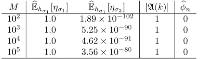
M Ehσ₁[ησ1] Ehσ1[ησ2] |A(k)| φn 102 1.0 1.89×10−102 1 0 103 1.0 5.25×10−90 1 0 104 1.0 4.62×10−91 1 0 105 _{1.0 3.56×10}−80 _{1 0}

Table 1: Estimates for {Ehσ₁[ησi]}k!i=1, |A(k)| and φn against M for D1 (k = 2). The prior for a variance parameter isIG(2,3). Note thatEhσ₁[ησ1] = 1 due to rounding.

M Ehσ₁[ησ1] Ehσ₁[ησ2] Ehσ₁[ησ3] Ehσ₁[ησ4] Ehσ₁[ησ5] Ehσ₁[ησ6] |A(k)| φn 102 _{1.0 3.56×10}−16 _5.05×10−55 _4.64×10−65 _8.27×10−144 _9.53×10−160 _{2 0} 103 1.0 1.22×10−8 3.01×10−49 2.27×10−53 3.08×10−125 1.11×10−144 2 0 104 _{1.0 2.03×10}−8 _1.76×10−43 _4.87×10−49 _2.61×10−95 _8.31×10−136 _{2 0} 105 1.0 1.04×10−5 2.27×10−39 1.51×10−44 4.30×10−87 1.56×10−122 2 0 Table 2: Estimates for {Ehσ₁[ηi]}k!i=1,|A(k)|and φn with respect toM forD2 (k= 3). The prior for a variance parameter isIG(2,15). Note thatEhσ₁[ησ1] = 1 due to rounding errors.

The expected relative contribution measures for D1 and D2 are given in Tables 1 and 2, respectively. For J = 102 initial Gibbs simulations, significantly contributing clusters are easily identified by (Ehσ1[ησi(θ)])

k!

i=1, and both|A(k)| andφare relatively stable againstM. Under a natural lack of label switching,q(θ) seems to be well approx-imated using onlyhσ1(θ), as seen in Table1. Even when some label switching occurs in a Gibbs sequence corresponding to a Gaussian mixture model with three components, only two terms,hσ1(θ) andhσ2(θ), significantly contribute toq(θ), as seen in Table2. For the subsequent analyses in this paper, we choseJ = 102_{,M = 10}3 _{andτ = 10}−324_.

5.2

Simulation results

The following seven marginal likelihood estimators using an equal number of proposals are compared:

E∗_Ch Chib’s method (2) using T = 104 _{samples and multiplying by k! to compensate} for lack of label switching;

ECh Chib’s method (2), usingT = 104randomly permuted Gibbs samples;

EIS Importance sampling using q as in (6), with a maximum likelihood estimate for

zo

1, . . . , zno andT = 104 particles;

EDS Dual importance sampling usingq as in (7), with T = 104 particles and J = 100 Gibbs samples inq(θ);

EA_DS Dual importance sampling using an approximation as in (13), with T = 104 par-ticles,J = 100 andM = 103_;

EJ1 Importance sampling usingqas in (4) withT = 10

4_{particles andJ}

1= 100k! Gibbs samples inq;

EBS Bridge sampling (3), using M1=M2= 5×103 samples andq(θ) as in (4) via 10 iterations. Label switching is imposed in hyperparameters{θ(j), z(j)_}J1

j=1 inqand

J1= 100k!.

The marginal likelihood estimates (in log-scales) and the effective sample size (ESS) ratios, R = ESS/T, are summarised in Figures 2 and 3 by boxplots, based on 50 replicates. Subscripts ofEandRdenote the estimating technique. Note that a modified ESS, provided by (35) in Doucet et al. (2000), is used here for numerical stability. All estimators are based on 104_{proposals, as in Table3, where summing up the second and} third columns leads to a fixed total number of function evaluations. Within our setup,

EIS is the least demanding in terms of computational workload while the remaining importance estimators require the same workload, except for EA_DS.

Simulated mixture datasets

Mixture models of two and three components are fitted to D1 and D2, respectively. Regardless of the presence or absence of label switching in the resulting Gibbs sequences, all estimates based on importance sampling exceptEIS coincide withECh, albeit with possibly smaller Monte Carlo variations as seen in Figures2and 3and Table4. When a suitable approximate forq(θ) is used for the dual importance sampling, no significant difference in the estimates and the effective sample sizes is observed. The mean sizes ofA(k) in Table 5are always smaller than k! and it shows thatE(k) can be estimated with a lesser computational workload. When posterior modes are very well separated (no natural label switching ever present in Gibbs sequences), the number of evaluations inq

is reduced almost by the maximal factor of 1/k!. Computing time increases by a factor of k! with k for most importance sampling based estimators in Table 6 and increases relatively slowly for Chib’s methods. Overall,EBS requires the highest computing time.

Estimate Number of posterior Number of marginal posterior Number of proposals evaluations density evaluations inq

E_IS T T k! T EDS T T J k! T EA_DS T (M+ (T−M)|A(k)|/k!)J k! T EJ1 T T J1 T EBS M1 (M1+M2)J1 M1+M2

Table 3: Computation steps required by different evidence estimation approaches. Note that the required computation forEBS includes 10 iterations.

Figure 2: Boxplots of evidence estimates in log-scale(left, middle)and effective sample sizes ratios(right). Mixture models with two and three Gaussian components are fitted to (top) D1 and(bottom) D2, respectively. The prior for {σ2i}ki=1 isIG(2,3) and label switching did not occur in Gibbs samples. One outlier of E_IS in the top-left panel is discarded.

Figure 3: Boxplots of evidence estimates in log-scale(left, middle)and effective sample sizes ratios(right). Mixture models with two and three Gaussian components are fitted to(top) D1and(bottom)D2, respectively. The prior for{σi2}ki=1 isIG(2,15) and label switching naturally occurred in Gibbs samples. Two outliers for E∗_Ch in the top-left panel are discarded.

Figure 4: Boxplots of evidence estimates in log-scale(left, middle)and effective sample sizes ratios(right). Mixture models with three and four Gaussian components are fitted to (top) D1 and (bottom)D2, respectively. The prior for {σ2i}ki=1 isIG(2,3) and label switching occurs due to an extra component.

Data p(σ2_{) k E}ˆ IS ˆE∗Ch EˆCh ˆEDS EˆADS ˆEJ1 EˆBS D1 IG(2,3) 2 −158.0896 −158.0484 −158.0594 −158.0578 −158.0575 −158.0568 −158.0563 IG(2,15) 2 −160.5695 −159.8051 −160.3762 −160.3689 −160.3700 −160.3618 −160.3721 IG(2,3) 3 −160.3487 −156.8313 −158.1181 −158.1823 −158.1732 −158.1833 −158.2115 D2 IG(2,3) 3 −224.0944 −223.9207 −223.9379 −223.9285 −223.9229 −223.9279 −223.9323 IG(2,15) 3 −231.6750 −230.5445 −231.1845 −231.1876 −231.1902 −231.1539 −231.2115 IG(2,3) 4 −225.1238 −220.9748 −223.3749 −223.6071 −223.5916 −223.5936 −223.6009

Table 4: Average values for 50 estimates for E(k) per estimator.

WhenA(k)< k!, some reduction in the computing time of E(k)A

DS is observed and is due to ignoring zero function evaluations.

The above study considers the case when a mixture model is not overfitted, i.e. does not have superfluous components, and when label switching does not necessarily occur. In the event a mixture model is overfitted, label switching always occurs due to those extra (and unnecessary) components in a mixture representation. However, this does not mean that we cannot transform conditional densities associated with each ofhσ’s to be closer, resorting to a label switching removal technique. For instance, mixture models with three and four components were fitted to the datasets D1 and D2, respectively. For those overfitted mixtures, performance phenomena similar to the above study are again observed in Figure4 and Table4;E∗_Ch andE_IS are quite off from the remaining estimators; an approximate set size |A(k)|remains smaller than k! in Table5 and the corresponding computing time is reduced as shown by Table6.

Disagreement in the values ofEIS versusEChshows that an importance function may (unsurprisingly) fail to properly approximate pk(x|θ)πk(θ), resulting in an unreliable

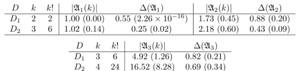
D k k! |A1(k)| Δ(A1) |A2(k)| Δ(A2) D1 2 2 1.00 (0.00) 0.55 (2.26×10−16) 1.73 (0.45) 0.88 (0.20) D2 3 6 1.02 (0.14) 0.25 (0.02) 2.18 (0.60) 0.43 (0.09) D k k! |A3(k)| Δ(A3) D1 3 6 4.92 (1.26) 0.82 (0.21) D2 4 24 16.52 (8.28) 0.69 (0.34)

Table 5: Mean and standard deviation(values in brackets)estimates for the approxima-tion set size,|A(k)|, and the reduction rate of a number of evaluatedh-terms, Δ(A), as in (15) forD1andD2. Subscripts 1 and 2 indicate results using the priorsσ2∼IG(2,3) andσ2∼IG(2,15), respectively. Estimates using overfitted models (σ2∼IG(2,3)) are indicated by the subscript 3.

D1 D2 Estimator T1 T2 T3 T1 T2 T3 E∗_Ch 0.64 0.91 1.01 1.19 1.22 1.50 ECh 0.64 0.70 0.99 1.09 1.09 1.56 EIS 0.06 0.06 0.54 0.61 0.62 0.63 EDS 0.52 0.51 1.56 1.73 1.67 7.06 EA_DS 0.40 0.56 1.53 0.86 1.08 3.54 EJ1 0.48 0.47 1.97 2.05 1.83 9.10 E_BS 0.87 0.84 2.49 2.42 2.38 10.75

Table 6: Elapsed time in seconds for evidence approximations in mixture models for

D1andD2using a 2.5 GHz Intel Core i5 processor. Subscripts 1 and 2 ofT indicate results using the priors σ2 _{∼ IG(2,3) and σ}2 _{∼ IG(2,15), respectively. Computing} times for overfitted models (σ2∼IG(2,3)) are indicated by the subscript 3.

estimate with large variation. Significantly small effective sample sizes (i.e. very small values forRIS) back this observation. When label switching naturally occurs, as in the Gibbs sequence (either under the variance priorIG(2,15) or due to extra components),

E∗_Ch disagrees with the other estimates, see Figures 3 and4. Also unsurprisingly, this indicates that the simplistic correction through a multiplication by k! is of no use, as reported in Neal (1999), Fr¨uhwirth-Schnatter (2006) and Marin and Robert (2008). Galaxy and fishery datasets

The priors suggested by Richardson and Green (1997) are used for our simulation study:

μ1, . . . , μk ∼ N(¯x, r2/4),

σ2

1, . . . , σ2k ∼ IG(2, β),

β ∼ G(0.2,10/r2_),

λ1, . . . , λk ∼ Dirichlet(1, . . . ,1)

where ¯xandrare the median and the range ofx, respectively. Normal mixture models are fitted to both datasets and estimates of log(E(k)) and R are summarised in

Fig-Figure 5: Simulation result for the galaxy dataset. Boxplots of evidence estimates in log-scale(left, middle)and effective sample sizes ratios(right). Mixture models with(top) three, (middle) four, and (bottom)six Gaussian components are fitted. One outlier of

ECh in the top-left panel is discarded.

Data k ˆEIS Eˆ∗_Ch EˆCh EˆDS EˆADS EˆJ1 EˆBS Fishery data 3 −519.6454 −519.3633 −519.5993 −519.3584 −519.3630 −519.4073 −519.3718 4 −518.1560 −515.9706 −516.8680 −516.6662 −516.6196 −517.2511 −516.6378 Galaxy data 3 −225.8305 −225.5019 −225.4799 −225.4989 −225.5040 −225.5129 −225.4992 4 −224.9167 −222.3848 −223.9332 −224.0716 −224.0109 −224.0754 −224.1287 6 ₋226.1190 ₋221.0257 ₋223.1993 ₋222.7597 ₋222.5898 ₋222.7697 ₋222.7767

Table 7: Average values for 50 estimates for E(k) per estimator.

ures5and6and Table7. In general, a similar behaviour of log(E(k)) andRis observed between the methods. For all cases, the dual importance sampling schemes (EDS and

EA_DS), E_J1 and E_BS agree with Chib’s approach (E_Ch). Unless modes in joint poste-rior distributions are clearly separated (e.g. |A(k)| ≈1), log(E∗_Ch) is biased due to an improper permutation correction.EIS is quite off from other estimates, due to a poor support forq.

Symptoms of the “curse of dimensionality” are observed. Askincreases, the effective sample size decreases exponentially fast and the variation in the estimates increases. When k = 6, the variation in the estimates of ECh is much larger than those based on importance sampling and the approximation (EA_DS) with the current value forM is

Figure 6: Simulation result for the fishery dataset. Boxplots of evidence estimates in log-scale (left, middle) and effective sample sizes ratios (right). Mixture models with (top) three and(bottom) four Gaussian components are fitted. Two outliers ofECh in the top-left panel are discarded.

slightly biased. Bridge sampling provides relatively stable estimates against k. Due to the exponential increase ofk!, a fast increase in computing is observed for all estimators in Table8.

The reduction in numbers of evaluated terms used to approximateE(k) varies case by case, as shown in Table 9; the maximum reduction of 82% and the minimum of 57%. Particularly, a maximum computing time reduction of 59% compared to EBS is observed whenk= 4 and k= 6 (see Table8).

Estimator Fishery data Galaxy data

k= 3 k= 4 k= 3 k= 4 k= 6 E∗_Ch 1.16 1.54 1.06 1.68 2.13 ECh 1.18 1.61 1.05 1.88 7.19 EIS 0.33 0.58 0.16 0.92 7.83 E_DS 1.91 8.47 1.74 8.61 396.81 EA_DS 1.74 6.51 1.54 6.41 245.95 EJ1 2.32 14.85 2.32 10.67 530.54 EBS 2.82 13.79 2.76 12.53 610.18

Table 8: Elapsed time in seconds for evidences approximation of mixture models for fishery and galaxy datasets using a 2.5 GHz Intel Core i5 processor.

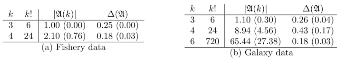
k k! |A(k)| Δ(A) 3 6 1.00 (0.00) 0.25 (0.00) 4 24 2.10 (0.76) 0.18 (0.03)

(a) Fishery data

k k! |A(k)| Δ(A)

3 6 1.10 (0.30) 0.26 (0.04) 4 24 8.94 (4.56) 0.43 (0.17) 6 720 65.44 (27.38) 0.18 (0.03)

(b) Galaxy data

Table 9: Mean and standard deviation (values in brackets) of approximate set sizes,

|A(k)|, and the reduction rate of a number of evaluatedh-terms Δ(A) as in (15) for (a) fishery and (b) galaxy datasets.

6

Discussion

This paper considered evidence approximations by importance sampling for mixture models and re-evaluated some of the known challenges resulting from high multimodality in a posterior density. Importance sampling requires that the support of an importance function encompasses the support of a posterior density to perform properly. In the specific case of mixture models, missing some of modes in a posterior distribution is likely to produce an unsuitable support, hence a poor estimate of the evidence.

In our experiments, exchangeable priors are used and the posterior density ex-hibitsk! symmetrical terms. Two marginal likelihood estimators are proposed here and tested against other existing estimators. The first approach exploits the permutation of π(·|x,zo_{) with a point-wise MLE, z}o_{, to create an importance function. However,} due to a poor resulting support, this approach performs quite poorly in our simulation studies. Another poor estimate is derived from Chib’s method when the invariance by permutation is not reproduced in the sample (Neal, 2001).

A second importance function is constructed by double Rao–Blackwellisation, hence the denomination ofdual importance sampling. We demonstrate both methodologically and practically that this solution fits the demands of evidence estimation for mixture models. Moreover, introducing a suitable and implementable approximation scheme, we show how to reduce the exponential increase in computational workload. The core idea of this approximation is to bypass negligible elements in the approximation thanks to the perfect symmetry of a posterior density. When posterior modes are well-separated, the gain is of a larger magnitude than when those modes strongly overlap.

Borrowing from the original approach in Chib (1996), dual importance sampling can be extended to cases when conditional Gibbs sampling densities are not available in closed form. However, this solution suffers from the curse of dimensionality, just like any other importance sampling estimator.

Alternative evidence approximation techniques could as well be considered for this problem, as exemplified in Friel and Wyse (2012). For instance, ensemble Monte Carlo samples from local ensembles that are extensions or compositions of the original, e.g. us-ing parallel temperus-ing Monte Carlo methods. Extendus-ing this idea, Bayes factor approx-imations were proposed using annealed importance sampling (Neal, 2001) and power posteriors (Friel and Pettitt,2008). Further investigation is needed to characterise the performances of those alternative solutions in the setting of mixture models and label switching.

References

Antoniak, C. (1974). “Mixtures of Dirichlet processes with applications to Bayesian nonparametric problems.” The Annals of Statistics, 2: 1152–1174.MR0365969. 3 Ardia, D., Ba¸st¨urk, N., Hoogerheide, L., and van Dijk, H. K. (2012). “A

compar-ative study of Monte Carlo methods for efficient evaluation of marginal likeli-hood.” Computational Statistics and Data Analysis, 56: 3398–3414. MR2943902. doi:http://dx.doi.org/10.1016/j.csda.2010.09.001. 3

Berkhof, J., Mechelen, I. v., and Gelman, A. (2003). “A Bayesian approach to the selec-tion and testing of mixture models.”Statistical Sinica, 13(3): 423–442.MR1977735. 3,4,6

Carlin, B. and Chib, S. (1995). “Bayesian model choice through Markov chain Monte Carlo.” Journal of the Royal Statistical Society: Series B (Statistical Methodology), 57(3): 473–484. 3

Celeux, G., Hurn, M., and Robert, C. P. (2000). “Computational and inferential diffi-culties with mixture posterior distributions.”Journal of the American Statistical As-sociation, 95(3): 957–979. MR1804450. doi:http://dx.doi.org/10.2307/2669477. 2

Chen, M.-H., Shao, Q. M., and Ibrahim, J. G. (2000). Monte Carlo Methods in Bayesian Computation. Springer Series in Statistics, first edition. MR1742311. doi:http://dx.doi.org/10.1007/978-1-4612-1276-8. 5

Chib, S. (1995). “Marginal likelihoods from the Gibbs output.”Journal of the American Statistical Association, 90: 1313–1321.MR1379473. 3, 4,12

— (1996). “Calculating posterior distributions and modal estimates in Markov mixture models.” Journal of Econometrics, 75: 79–97. MR1414504. doi:http://dx.doi.org/10.1016/0304-4076(95)01770-4. 3,20

Chopin, N. (2002). “A sequential particle filter method for static models.”Biometrika, 89(3): 539–552. MR1929161. doi: http://dx.doi.org/10.1093/biomet/89.3.539. 4

Chopin, N. and Robert, C. P. (2010). “Properties of nested sampling.”Biometrika, 97: 741–755. MR2672495. doi:http://dx.doi.org/10.1093/biomet/asq021. 3,4 Congdon, P. (2006). “Bayesian model choice based on Monte Carlo estimates of

poste-rior model probabilities.” Computational Statistics and Data Analysis, 50: 346–357. MR2201867. doi:http://dx.doi.org/10.1016/j.csda.2004.08.001. 3

DiCiccio, A. P., Kass, R. E., Raftery, A., and Wasserman, L. (1997). “Com-puting Bayes factors by combining simulation and asymptotic approximations.” Journal of the American Statistical Association, 92: 903–915. MR1482122. doi:http://dx.doi.org/10.2307/2965554. 3

Diebolt, J. and Robert, C. (1994). “Estimation of finite mixture distributions through Bayesian sampling.” Journal of the Royal Statistical Society: Series B (Statistical Methodology), 56: 363–375.MR1281940. 2

Doucet, A., Godsill, S., and Andrieu, C. (2000). “On sequential Monte Carlo sampling methods for Bayesian filtering.”Statistics and Computing, 10: 197–208. 14

Escobar, M. and West, M. (1995). “Bayesian density estimation and inference us-ing mixtures.” Journal of the American Statistical Association, 90(430): 577–588. MR1340510. 3

Friel, N. and Pettitt, A. N. (2008). “Marginal likelihood estimation via power pos-teriors.” Journal of the Royal Statistical Society: Series B (Statistical Methodol-ogy), 70: 589–607. MR2420416. doi: http://dx.doi.org/10.1111/j.1467-9868. 2007.00650.x. 20

Friel, N. and Wyse, J. (2012). “Estimating the evidence: a review.” Statistica Neer-landica, 66(3): 288–308. MR2955421. doi: http://dx.doi.org/10.1111/j.1467-9574.2011.00515.x. 20

Fr¨uhwirth-Schnatter, S. (2001). “Markov Chain Monte Carlo estimation for classi-cal and dynamic switching and mixture models.” Journal of the American Sta-tistical Association, 96: 194–209. MR1952732. doi: http://dx.doi.org/10.1198/ 016214501750333063. 1,2,5

— (2004). “Estimating marginal likelihoods for mixture and Markov switching models using bridge sampling techniques.”Journal of Econometrics, 7: 143–167. MR2076630. doi:http://dx.doi.org/10.1111/j.1368-423X.2004.00125.x. 5,6

Fr¨uhwirth-Schnatter, S. (2006).Finite Mixture and Markov Switching Models. Springer Series in Statistics, first edition.MR2265601. 6,12,17

— (2008). bayesf : Finite Mixture and Markov Switching Models. MAT-LAB package version 2.0.http://statmath.wu.ac.at/ fruehwirth/monographie/

book matlab version 2.0.pdf 6

Gelfand, A. E. and Smith, A. F. M. (1990). “Sampling-based approaches to calculating marginal densities.” Journal of the American Statistical Association, 85: 398–409. MR1141740. 3,4

Gelman, A. and Meng, X. L. (1998). “Simulating normalizing constants: From impor-tance sampling to bridge sampling to path sampling.”Statistical Science, 13: 163–185. MR1647507. doi:http://dx.doi.org/10.1214/ss/1028905934. 3,5

Geweke, J. (2012). “Interpretation and inference in mixture models: simple MCMC works.” Computational Statistics and Data Analysis, 51: 3529–3550. MR2367818. doi:http://dx.doi.org/10.1016/j.csda.2006.11.026. 2

Green, P. (1995). “Reversible jump Markov chain Monte Carlo computation and Bayesian model determination.” Biometrika, 85(4): 711–732. MR1380810. doi:http://dx.doi.org/10.1093/biomet/82.4.711. 4

Jasra, A., Holmes, C., and Stephens, D. (2005). “Markov Chain Monte Carlo methods and the label switching problem in Bayesian mixture modeling.” Statistical Science, 20(1): 50–67. MR2182987. doi:http://dx.doi.org/10.1214/088342305000000016. 2,11,12

Jeffreys, H. (1939). Theory of Probability. Oxford, The Clarendon Press, first edition. 3

Marin, J. and Robert, C. (2007). Bayesian Core. Springer-Verlag, New York. MR2723361. 2

— (2010a). “Importance sampling methods for Bayesian discrimination between em-bedded models.” In: Chen, M.-H., Dey, D., M¨uller, P., Sun, D., and Ye, K. (eds.), Frontiers of Statistical Decision Making and Bayesian Analysis. Springer-Verlag, New York. 3

— (2010b). “On resolving the Savage–Dickey paradox.”Electronic Journal of Statistics, 4: 643–654. MR2660536. doi:http://dx.doi.org/10.1214/10-EJS564. 3

Marin, J.-M., Mengersen, K., and Robert, C. P. (2005). “Bayesian modelling and infer-ence on mixtures of distributions.” In: Rao, C. and Dey, D. (eds.),Handbook of Statis-tics, volume 25. Springer-Verlag, New York. MR2490536. doi:http://dx.doi.org/ 10.1016/S0169-7161(05)25016-2. 1

Marin, J.-M. and Robert, C. P. (2008). “Approximating the marginal likelihood in mixture models.”Bulletin of the Indian Chapter of ISBA, 1: 2–7. 3,6,17

Meng, X. L. and Schilling, S. (2002). “Warp Bridge sampling.” Journal of Computa-tional Graphical Statistics, 11(3): 552–586. MR1938446. doi: http://dx.doi.org/ 10.1198/106186002457. 3,5

Meng, X. L. and Wong, W. H. (1996). “Simulating ratios of normalizing constants via a simple identity.”Statistica Sinica, 6: 831–860.MR1422406. 3,5

Mira, A. and Nicholls, G. (2004). “Bridge estimation of the probability density at a point.”Statistica Sinica, 14: 603–612.MR2059299. 5

Neal, R. M. (1999). “Erroneous results in Marginal likelihood from the Gibbs output.” http://www.cs.toronto.edu/~radford/chib-letter.html 3, 4,17

— (2001). “Annealed importance sampling.” Statistics and Computing, 11: 125–139. MR1837132. doi:http://dx.doi.org/10.1023/A:1008923215028. 20

Newton, M. A. and Raftery, A. E. (1994). “Approximate Bayesian inference with the weighted likelihood bootstrap.” Journal of the Royal Statistical Society: Series B (Statistical Methodology), 96(1): 3–48. MR1257793. 3

Papastamoulis, P. (2013).label.switching: Relabelling MCMC outputs of mixture models. R package version 1.2. http://CRAN.R-project.org/package=label.switching 2

Papastamoulis, P. and Iliopoulos, G. (2010). “An artificial allocations based solution to the label switching problem in Bayesian analysis of mixtures of distributions.” Journal of Computational and Graphical Statistics, 19(2): 313–331. MR2758306. doi:http://dx.doi.org/10.1198/jcgs.2010.09008. 2, 11

Papastamoulis, P. and Roberts, G. (2008). “Retrospective Markov chain Monte Carlo methods for Dirichlet process hierarchical models.” Biometrika, 95: 315–321. MR2409721. doi:http://dx.doi.org/10.1093/biomet/asm086. 2

Perrakis, K., Ntzoufras, I., and Tsionas, E. G. (2014). “On the use of marginal pos-teriors in marginal likelihood estimation via importance sampling.” Computational Statistics and Data Analysis, 77: 54–69. MR3210048. doi: http://dx.doi.org/ 10.1016/j.csda.2014.03.004. 6

Raftery, A., Newton, M., Satagopan, J., and Krivitsky, P. (2006). “Estimating the inte-grated likelihood via posterior simulation using the harmonic mean identity.” Tech-nical Report 499, University of Washington, Department of Statistics. MR2433201. 3

Rasmussen, C. E. (2000). “The Infinite Gaussian Mixture Model.” In: Advances in Neural Information Processing Systems 12, 554–560. MIT Press. 3

Richardson, S. and Green, P. (1997). “On Bayesian analysis of mixtures and with an unknown number of components.” Journal of the Royal Statistical Society: Series B (Statistical Methodology), 59(4): 731–792. MR1483213. doi:http://dx.doi.org/ 10.1111/1467-9868.00095. 2,3,4, 12, 17

Robert, C. and Marin, J.-M. (2008). “On some difficulties with a posterior proba-bility approximation technique.” Bayesian Analysis, 3(2): 427–442. MR2407433. doi:http://dx.doi.org/10.1214/08-BA316. 3

Robert, C. P. and Casella, G. (2004).Monte Carlo Statistical Methods. Springer, second edition. MR2080278. doi:http://dx.doi.org/10.1007/978-1-4757-4145-2. 2,4 Rodriguez, C. and Walker, S. (2014). “Label switching in Bayesian mixture mod-els:Deterministic relabeling strategies.” Journal of Computational and Graphical Statistics, 21(1): 23–45. MR3173759. doi:http://dx.doi.org/10.1080/10618600. 2012.735624. 2,11

Rubin, D. B. (1987). “Comment on “The calculation of posterior distributions by data augmentation” by M. A. Tanner and W. H. Wong.”Journal of the American Statis-tical Association, 82: 543–546.MR0898357. 3

— (1988). “Using the SIR algorithm to simulate posterior distributions.” In: Bernardo, J. M., DeGroot, M. H., Lindley, D. V., and Smith, A. F. M. (eds.),Bayesian Statistics, 3, 395–402. Oxford University Press. 3

Satagopan, J., Newton, M., and Raftery, A. (2000). “Easy Estimation of Normalizing Constants and Bayes Factors from Posterior Simulation: Stabilizing the Harmonic Mean Estimator.” Technical Report 1028, University of Wisconsin-Madison, Depart-ment of Statistics. 3

Scott, S. L. (2002). “Bayesian methods for hidden Markov models: recursive computing in the 21st Century.” Journal of the American Statistical Association, 97: 337–351. MR1963393. doi:http://dx.doi.org/10.1198/016214502753479464. 3

Servidea, J. D. (2002). “Bridge sampling with dependent random draws: techniques and strategy.” Ph.D. thesis, Department of Statistics, The University of Chicago. MR2717042. 5

Skilling, J. (2007). “Nested sampling for Bayesian computations.” Bayesian Analysis, 1(4): 833–859. MR2282208. doi: http://dx.doi.org/10.1214/06-BA127. 4