A global homogeneity test for high-dimensional linear
regression
Camille Charbonnier, Nicolas Verzelen, Fanny Villers
To cite this version:
Camille Charbonnier, Nicolas Verzelen, Fanny Villers. A global homogeneity test for
high-dimensional linear regression. Electronic journal of statistics , Shaker Heights, OH : Institute
of Mathematical Statistics, 2015, 9 (1), pp.318-382.
<
10.1214/15-EJS999
>
.
<
hal-01263375
>
HAL Id: hal-01263375
http://hal.upmc.fr/hal-01263375
Submitted on 27 Jan 2016
HAL
is a multi-disciplinary open access
archive for the deposit and dissemination of
sci-entific research documents, whether they are
pub-lished or not.
The documents may come from
teaching and research institutions in France or
abroad, or from public or private research centers.
L’archive ouverte pluridisciplinaire
HAL, est
destin´
ee au d´
epˆ
ot et `
a la diffusion de documents
scientifiques de niveau recherche, publi´
es ou non,
´
emanant des ´
etablissements d’enseignement et de
recherche fran¸
cais ou ´
etrangers, des laboratoires
publics ou priv´
es.
Vol. 9 (2015) 318–382 ISSN: 1935-7524 DOI:10.1214/15-EJS999
A global homogeneity test
for high-dimensional linear
regression
Camille CharbonnierInserm U1079, CNR-MAJ Rouen University Hospital 22 boulevard Gambetta
76183 Rouen, France
e-mail:[email protected] Nicolas Verzelen
INRA, UMR 729 MISTEA 2 Place Viala, B ˆAT. 29 F-34060 Montpellier, France e-mail:[email protected]
and Fanny Villers
LPMA, University Pierre et Marie Curie 4 place Jussieu
75005 Paris, France e-mail:[email protected]
Abstract: This paper is motivated by the comparison of genetic networks inferred from high-dimensional datasets originating from high-throughput Omics technologies. The aim is to test whether the differences observed between two inferred Gaussian graphical models come from real differences or arise from estimation uncertainties. Adopting a neighborhood approach, we consider a two-sample linear regression model with random design and propose a procedure to test whether these two regressions are the same. Relying on multiple testing and variable selection strategies, we develop a testing procedure that applies to high-dimensional settings where the number of covariatesp is larger than the number of observations n1 and
n2 of the two samples. Both type I and type II errors are explicitly
con-trolled from a non-asymptotic perspective and the test is proved to be minimax adaptive to the sparsity. The performances of the test are evalu-ated on simulevalu-ated data. Moreover, we illustrate how this procedure can be used to compare genetic networks on Hesset al.breast cancer microarray dataset.
AMS 2000 subject classifications:Primary 62H15; secondary 62P10.
Keywords and phrases:Gaussian graphical model, two-sample hypoth-esis testing, high-dimensional statistics, multiple testing, adaptive testing, minimax hypothesis testing, detection boundary.
Received August 2013.
1. Introduction
The recent flood of high-dimensional data has motivated the development of a vast range of sparse estimators for linear regressions, in particular a large variety of derivatives from the Lasso. Although theoretical guarantees have been provided in terms of prediction, estimation and selection performances (among a lot of others [6, 36, 50]), the research effort has only recently turned to the construction of high-dimensional confidence intervals or parametric hypothesis testing schemes [7, 25,31,33,52]. Yet, quantifying the confidence surrounding coefficient estimates and selected covariates is essential in areas of application where these will nourish further targeted investigations.
In this paper we consider the two-sample linear regression model with Gaus-sian random design.
Y(1) = X(1)β(1)+(1) (1)
Y(2) = X(2)β(2)+(2). (2)
In this statistical model, the size prow vectorsX(1) andX(2) follow Gaussian distributionsN(0p,Σ(1)) andN(0p,Σ(2)) whose covariance matrices remain
un-known. The noise components (1) and (2) are independent from the design matrices and follow a centered Gaussian distribution with unknown standard deviationsσ(1)andσ(2). In this formal setting, our objective is to develop a test for the equality ofβ(1) andβ(2) which remains valid in high-dimension.
Suppose that we observe an n1-sample of (Y(1), X(1)) and an n2-sample of (Y(2), X(2)) notedY(1),X(1), andY(2),X(2), withn
1andn2remaining smaller thanp. Defining(1)and(2)analogously, we obtain the decompositionsY(1)=
X(1)β(1)+(1) and Y(2) =X(2)β(2)+(2). Given these observations, we want to test whether models (1) and (2) are the same, that is
(
H0: β(1)=β(2), σ(1) =σ(2), and Σ(1)= Σ(2)
H1: β(1)6=β(2) or σ(1)6=σ(2).
(3) In the null hypothesis, we include the assumption that the population covari-ances of the covariates are equal (Σ(1) = Σ(2)), whereas under the alternative hypothesis the population covariances are not required to be the same. This choice of assumptions is primarily motivated by our final objective to derive homogeneity tests for Gaussian graphical models (see below). A discussion of the design hypotheses is deferred to Section7.
1.1. Connection with two-sample Gaussian graphical model testing
This testing framework is mainly motivated by the validation of differences observed between Gaussian graphical models (modelling regulation networks) inferred from high-throughput Omics data from two samples [12,18,34] when looking for new potential drug or knock-out targets [26]. Following the devel-opment of univariate differential analysis techniques, there is now a surging
demand for the detection of differential regulations between pairs of conditions (treated vs. placebo, diseased vs. healthy, exposed vs. controls . . . ).
The special case when the structure of the network itself is known and only edge weights between genes have to be estimated has already been addressed by the literature (e.g. [41]). Only a few papers have tackled the issue of com-paring two estimated networks, facing the difficulty of disentangling estimation errors from true differences in the underlying networks. A first attempt at solv-ing this problem can be found in [19]. Assuming the issue of high-dimensional network estimation solved by use of correlations, regularized partial correlations or partial least square estimation, the authors defined three measures of the dif-ferences between networks either in terms of modularity changes or of average edge weights between genes. Another work [13] derived a testing strategy from empirical Bayes posterior distributions of edge weights. However, none of these two papers provide theoretical guarantees on type-I error control or on detection properties of the suggested methods, in particular in a high-dimensional context. We suggest to build upon our two-sample high-dimensional linear regression testing scheme to derive a global test for the equality of Gaussian graphical mod-els inferred under pairs of conditions. We keep in mind our two main objectives: meeting the practical challenges associated with high-dimension and character-izing the performances of our procedure from a theoretical point of view.
Formally speaking, the global two-sample GGM testing problem is defined as follows. Consider two Gaussian random vectors Z(1)
∼ N(0,[Ω(1)]−1) and
Z(2)
∼ N(0,[Ω(2)]−1). The conditional independence graphs are characterized by the non-zero entries of the precision matrices Ω(1) and Ω(2) [28]. Given an
n1-sample ofZ(1) and ann2-sample ofZ(2), the objective is to test
HG
0 : Ω(1)= Ω(2) versus HG1 : Ω(1)6= Ω(2), (4) where Ω(1) and Ω(2) are assumed to be sparse (most of their entries are zero). This testing problem is global as the objective is to assess a statistically sig-nificant difference between the two distributions. If the test is rejected, a more ambitious objective is to infer the entries where the precision matrices differ (i.e. Ω(1)i,j 6= Ω(2)i,j).
Adopting a neighborhood selection approach [34] as recalled in Section 6, high-dimensional GGM estimation can be solved by multiple high-dimensional linear regressions. As such, two-sample GGM testing (4) can be solved via mul-tiple two-sample hypothesis testing as (3) in the usual linear regression frame-work. This extension of two-sample linear regression tests to GGMs is described in Section6.
1.2. Related work
The literature on high-dimensional two-sample tests is very light. In the con-text of high-dimensional two-sample comparison of means, [3,11, 32, 42] have introduced global tests to compare the means of two high-dimensional Gaussian vectors with unknown variance. Recently, [8,29] developed two-sample tests for covariance matrices of two high-dimensional vectors.
In contrast, the one-sample analog of our problem has recently attracted a lot of attention, offering as many theoretical bases for extension to the two-sample problem. In fact, the high-dimensional linear regression tests for the nullity of coefficients can be interpreted as a limit of the two-sample test in the case where
β(2) is known to be zero, and the sample size n
2 is considered infinite so that we perfectly know the distribution of the second sample.
There are basically two different objectives in high-dimensional linear test-ing: a local and a global approach. In the local approach, one considers the p
tests for the nullity of each coefficient H0,i : βi(1) = 0 (i = 1, . . . , p) with the
purpose of controlling error measures such as the false discovery rate of the re-sulting multiple testing procedures. In a way, one aims to assess the individual statistical significance of each of the variables. This can be achieved by provid-ing a confidence region forβ(1) [7,25,31, 33,52]. Another line of work derives
p-values for the nullity of each of the coefficients. Namely, [51] suggests a screen and clean procedure based upon half-sampling. Model selection is first applied upon a random half of the sample in order to test for the significance of each coefficient using the usual combination of ordinary least squares and Student t-tests on a model of reasonable size on the remaining second half. To reduce the dependency of the results to the splitting, [35] advocate to use half-samplingB
times and then aggregate theB p-values obtained for variablej in a way which controls either the family-wise error rate or false discovery rate.
In the global approach, the objective is to test the null hypothesisH0: β(1)= 0. Although global approaches are clearly less informative than approaches pro-viding individual significance tests like [7, 35, 52], they can reach better per-formances from smaller sample sizes. Such a property is of tremendous im-portance when dealing with high-dimensional datasets. The idea of [49], based upon the work of [5], is to approximate the alternative H1 : β(1) 6= 0 by a collection of tractable alternatives {HS
1 : ∃j ∈ S, β (1)
j 6= 0, S ∈ S} working
on subsets S ⊂ {1, . . . , p} of reasonable sizes. The null hypothesis is rejected if the null hypothesis HS
0 is rejected for at least one of the subsets S ∈ S. Admittedly, the resulting procedure is computationally intensive. Nonetheless it is non-asymptotically minimax adaptive to the unknown sparsity of β(1), that is it achieves the optimal rate of detection without any assumption on the population covariance Σ(1) of the covariates. Another series of work relies on higher-criticism. This last testing framework was originally introduced in or-thonormal designs [16], but has been proved to reach optimal detection rates in high-dimensional linear regression as well [2,24]. In the end, higher-criticism is highly competitive in terms of computing time and achieves the asymptotic rate of detection with the optimal constants. However, these nice properties require strong assumptions on the design.
The testing strategy we describe in this paper is built upon the global ap-proach developed by [5] and [49].
While writing this paper, we came across the parallel work of St¨adler and Mukherjee, which deals similarly with both frameworks of two-sample linear regression [43] and two-sample graphical model comparison [44]. Their approach
shares the idea of sample-splitting and dimensionality reduction with thescreen and clean procedure in its simple-split [51] and multi-split [35] versions, in a global testing perspective however. A detailed comparison of [43, 44] with our contribution is deferred to simulations (Section5) and discussion (Section7).
1.3. Our contribution
Our suggested approach stems from the fundamental assumption that either the true supports ofβ(1)andβ(2) are sparse or their differenceβ(1)
−β(2) is sparse, so that the test can be successfully led in a subsetS?
⊂ {1, . . . , p}of variables
with reasonable size, compared to the sample sizesn1andn2. Of course, this low dimensional subsetS?is unknown. The whole objective of the testing strategy is
to achieve similar rates of detection (up to a logarithmic constant) as an oracle test that would know in advance the optimal low-dimensional subsetS?.
Concretely, we proceed in three steps:
1. We define algorithms to select a data-driven collection of subsetsSb iden-tified as most informative for our testing problem, in an attempt to cir-cumvent the optimal subsetS?.
2. New parametric statistics related to the likelihood ratio statistic between the conditional distributionsY(1)|XS(1)andY(2)|X
(2)
S are defined forS∈Sb.
3. We define two calibration procedures which both guarantee a control on type-I error:
• we use a Bonferroni calibration which is both computationally and conceptually simple, allowing us to prove that this procedure is min-imax adaptive to the sparsity ofβ(1)andβ(2)from a non-asymptotic point of view;
• we define a calibration procedure based upon permutations to reach a fine tuning of multiple testing calibration in practice, for an increase in empirical power.
The resulting testing procedure is completely data-driven and its type I error is explicitly controlled. Furthermore, it is computationally amenable in a largep
and smallnsetting.
The procedure is described in Section2while Section3is devoted to technical details, among which theoretical controls on Type I error, as well as some useful empirical tools for interpretation. Section4 provides a non-asymptotic control of the power. Section 5 provides simulated experiments comparing the perfor-mances of the suggested procedures with the approach of [43]. In Section 6, we detail the extension of the procedure to handle the comparison of Gaussian graphical models. The method is illustrated on Transcriptomic Breast Cancer Data. Finally, all the proofs are postponed to Section8.
TheRcodes of our algorithms are available athttp://www.proba.jussieu. fr/~villers/ as well as on the EJS website http://projecteuclid.org/ euclid.ejsas supplementary material of this paper [10].
1.4. Notation
In the sequel,`pnorms are denoted|·|p, except for thel2norm which is referred as k.k to alleviate notations. For any positive definite matrix Σ, k.kΣ denotes the Euclidean norm associated with the scalar product induced by Σ: for every vectorx,kxk2
Σ=x|Σx. Besides, for every setS, |S|denote its cardinality. For any integerk,Ik stands for the identity matrix of sizek. For any square matrix A,ϕmax(A) andϕmin(A) denote respectively the maximum and minimum eigen-values of A. When the context makes it obvious, we may omit to mentionA to alleviate notations and use ϕmax and ϕmin instead. Moreover, Y refers to the sizen1+n2concatenation ofY(1)andY(2)andXrefers to the size (n1+n2)×p concatenation ofX(1) andX(2). To finish with,Lrefers to a positive numerical constant that may vary from line to line.
2. Description of the testing strategy
Likelihood ratio statistics used to test hypotheses likeH0in the classicallargen, small psetting are intractable on high-dimensional datasets for the mere rea-son that the maximum likelihood estimator is not itself defined under high-dimensional design proportions. Our approach approximates the intractable high-dimensional test by a multiple testing construction, similarly to the strat-egy developed by [5] in order to derive statistical tests against non-parametric alternatives and adapted to one sample tests for high-dimensional linear regres-sion in [49].
For any subset S of {1, . . . , p} satisfying 2|S| ≤ n1∧n2, denote XS(1) and XS(2) the restrictions of random vectors X(1) and X(2) to covariates indexed byS. Their covariance structure is noted Σ(1)S (resp. Σ
(2)
S ). Consider the linear
regression ofY(1) ontoX(1) S defined by ( Y(1)=X(1) S β (1) S + (1) S Y(2)=X(2) S β (2) S + (2) S ,
where the noise variables(1)S and(2)S are independent fromXS(1) andXS(2) and follow centered Gaussian distributions with new unknown conditional standard deviationsσ(1)S andσS(2). We now state the test hypotheses in reduced dimension:
( H0,S : βS(1)=β (2) S , σ (1) S =σ (2) S , and Σ (1) S = Σ (2) S , H1,S : βS(1)6=βS(2) or σS(1)6=σS(2).
Of course, there is no reason in general forβS(1)andβS(2) to coincide with the restrictions ofβ(1) andβ(2) to S, even less in high-dimension since variables in
S can be in all likelihood correlated with covariates in Sc. Yet, as exhibited by
Lemma2.1, there is still a strong link between the collection of low dimensional hypothesesH0,S and the global null hypothesisH0.
Proof. UnderH0, the random vectors of sizep+ 1 (Y(1), X(1)) and (Y(2), X(2)) follow the same distribution. Hence, for any subsetS,Y(1)follows conditionally on XS(1) the same distribution as Y(2) conditionally on X(2)
S . In other words,
βS(1)=β(2)S .
By contraposition, it suffices to reject at least one of theH0,S hypotheses to
reject the global null hypothesis. This fundamental observation motivates our testing procedure. As summarized in Algorithm 1, the idea is to build a well-calibrated multiple testing procedure that considers the testing problemsH0,S
against H1,S for a collection of subsets S. Obviously, it would be prohibitive
in terms of algorithmic complexity to testH0,S for everyS ⊂ {1, . . . , p}, since
there would be 2p such sets. As a result, we restrain ourselves to a relatively
small collection of hypotheses{H0,S, S ∈S}b , where the collection of supports
b
S is potentially data-driven. If the collectionSbis judiciously selected, then we can manage not to lose too much power compared to the exhaustive search.
We now turn to the description of the three major elements required by our overall strategy (see Algorithm1):
1. a well-targeted data-driven collection of models Sbas produced by Algo-rithm2;
2. a parametric statistic to test the hypothesesH0,SforS∈Sb, we resort
ac-tually to a combination of three parametric statisticsFS,V,FS,1andFS,2;
3. a calibration procedure guaranteeing the control on type I error as in Algorithms3 or4.
2.1. Choices of test collections (step 1)
The first step of our procedure (Algorithm1) amounts to selecting a collectionSb
of subsets of{1, . . . , p}, also called models. A good collectionSbof subsets must satisfy a tradeoff between the inclusion of the maximum number of relevant subsets S and a reasonable computing time for the whole testing procedure, which is linear in the size|S|b of the collection. The construction ofSbproceeds in two steps: (i) One chooses a deterministic collection S of models. (ii) One defines an algorithm (calledModelChoicein Algorithm1) mapping the raw data (X,Y) to some collectionSbsatisfyingS ⊂ Sb . Even though the introduction of
S as an argument of the mapping could appear artificial at this point, this quantity will be used in the calibration step of the procedure. Our methodology can be applied to any fixed or data-driven collection. Still, we focus here on two particular collections. The first one is useful for undertaking the first steps of the mathematical analysis. For practical applications, we advise to use the second collection.
Deterministic collections like S≤k By deterministic, we mean that the
model choice step is trivial, in the sense thatModelChoice(X,Y,S) =S. Among deterministic collections, the most straightforward collections consist of all size-k
Algorithm 1Overall Adaptive Testing Strategy
Require: DataX(1),X(2),Y(1),Y(2), collectionSand desired levelα
Step 1 – Choose a collectionSbof low-dimensional models (as e.g.SbLassoin Algo-rithm2)
procedureModelChoice(X(1),X(2),Y(1),Y(2),S)
Define the model collectionS ⊂ Sb end procedure
Step 2 – Compute p-values for each test in low dimension procedureTest(X(1)S ,X (2) S ,Y (1),Y(2), b S)
foreach subsetSinSbdo
Compute the p-values ˜qV,S, ˜q1,S, ˜q2,Sassociated to the statisticsFS,V,FS,1,FS,2
end for end procedure
Step 3 – Calibrate decision thresholds as in Algorithms3(Bonferroni) or4 (Per-mutations)
procedureCalibration(X(1),X(2),Y(1),Y(2),
b
S,α)
foreach subsetSinSband eachi=V,1,2do
Define a thresholdαi,S.
end for end procedure Step 4 – Final Decision
if there is a least one model S inSbsuch that there is at least one p-value for which
˜
qi,S< αi,S then
Reject the global null hypothesisH0
end if
subsets of {1, . . . , p}, which we denoteSk. This kind of family provides
collec-tions which are independent from the data, thereby reducing the risk of over-fitting. However, as we allow the model size kor the total number of candidate variables p to grow, these deterministic families can rapidly reach unreason-able sizes. Admittedly, S1 always remains feasible, but reducing the search to models of size 1 can be costly in terms of power. As a variation on sizek mod-els, we introduce the collection of all models of size smaller than k, denoted
S≤k=Skj=1Sj, which will prove useful in theoretical developments.
Lasso-type collection SbLasso Among all data-driven collections, we
sug-gest the Lasso-type collection SbLasso. Before proceeding to its definition, let us informally discuss the subsets that a “good” collection Sb should contain. Let supp(β) denote the support of a vector β. Intuitively, under the alterna-tive hypothesis, good candidates for the subsets are either subsets of S∗
∨ :=
supp(β(1))
∪supp(β(2)) or subsets ofS∗
∆:= Supp(β(1)−β(2)). The first model
S∗ ∨ nicely satisfiesβ (1) S∗ ∨ =β (1) andβ(2) S∗ ∨ =β
(2). The second subset has a smaller size thanS∗
∨ and focuses on covariates corresponding to different parameters in the full regression. However, the divergence between effects might only appear conditionally on other variables with similar effects, this is why the first subset
S∗
∨ is also of interest. Obviously, both subsets S∨∗ andS∆∗ are unknown. This is why we consider a Lasso methodology that amounts to estimating bothS∗
∨ and
S∆∗ in the collection SbLasso. Concrete details on the construction ofSbLasso are postponed to Section3.1.
2.2. Parametric test statistic (step 2)
Given a subsetS, we consider the three following statistics to testH0,SagainstH1,S:
FS,V :=−2 + k Y(1)−X(1)βb(1)S k2/n 1 kY(2)−X(2)βb(2) S k2/n2 +kY (2) −X(2)βbS(2)k2/n 2 kY(1)−X(1)βb(1) S k2/n1 , (5) FS,1:= k X(2)S (βbS(1)−βbS(2))k2/n 2 kY(1)−X(1)βb(1) S k2/n1 , FS,2:=k X(1)S (βbS(1)−βb(2)S )k2/n 1 kY(2)−X(2)βb(2) S k2/n2 . (6)
As explained in Section3, these three statistics derive from the Kullback-Leibler divergence between the conditional distributionsY(1)|X(1)
S andY(2)|X
(2)
S . While
the first termFS,V evaluates the discrepancies in terms of conditional variances,
the last two termsFS,1 andFS,2address the comparison ofβ(1) toβ(2). Because the distributions of statisticsFS,i, for i=V,1,2, under the null
de-pend on the size ofS, the only way to calibrate the multiple testing step over a collection of models of various sizes is to convert the statistics to a unique com-mon scale. The most natural is to convert observed FS,i’s intop-values. Under H0,S, the conditional distributions ofFS,i fori=V,1,2 to XS are
parameter-free and explicit (see Proposition 3.1 in the next section). Consequently, one can define the exact p-values associated to FS,i, conditional on XS. However,
the computation of thep-values require a function inversion, which can be com-putationally prohibitive. This is why we introduce explicit upper bounds ˜qi,S
(Equations (14), (18)) of the exactp-values.
2.3. Combining the parametric statistics (step 3)
The objective of this subsection is to calibrate a multiple testing procedure based on the sequence ofp-values{(˜qV,S,q˜1,S,q˜2,S), S ∈S}b , so that the type-I error
remains smaller than a chosen levelα. In particular, when using a data-driven model collection, we must take good care of preventing the risk of overfitting which results from using the same dataset both for model selection and hypoth-esis testing.
For the sake of simplicity, we assume in the two following paragraphs that
∅*S, which merely means that we do not include in the collection of tests the
raw comparison of Var(Y(1)) to Var(Y(2)).
Testing procedure Given a model collection Sb and a sequence αb = (αi,S)i=V,1,2, S∈Sb, we define the test function:
Tbα b S = ( 1 if∃S ∈Sb, ∃i∈ {V,1,2} q˜i,S≤αi,S. 0 otherwise. (7)
In other words, the test function rejects the global null if there exists at least one model S ∈ Sbsuch that at least one of the three p-values is below the corresponding threshold αi,S. In Section3.3, we describe two methods to
ade-quately calibrate thresholds (αi,S)S∈Sb. We first define a Bonferroni procedure,
whose conceptual simplicity allows us to derive non-asymptotic type II error bounds of the corresponding tests (Section4). However, this Bonferroni correc-tion reveals itself to be too conservative in practice, in part paying the price for resorting to data-driven collections and upper bounds on the true p-values. This is why we introduce as a second option the permutation calibration proce-dure. This second procedure controls the type I error at the nominal level and therefore outperforms the Bonferroni calibration in practice. Nevertheless, the mathematical analysis of the corresponding test becomes more intricate and we are not able to provide sharp type II error bounds.
Remark. In practice, we advocate the use of the Lasso Collection SbLasso (Algorithm2) combined with the permutation calibration method (Algorithm4). Henceforth, the corresponding procedure is denoted TP
b
SLasso.
3. Discussion of the procedure and type I error
In this section, we provide remaining details on the three steps of the testing procedure. First, we describe the collectionSbLassoand provide an informal justi-fication of its definition. Second, we explain the ideas underlying the parametric statisticsFS,i,i=V,1,2 and we define the correspondingp-values ˜qi,S. Finally,
the Bonferroni and permutation calibration methods are defined.
3.1. Collection SbLasso
We start fromS≤Dmax, where in practiceDmax=b(n1∧n2)/2c, and we consider the following reparametrized joint regression model.
Y(1) Y(2) = X(1) X(1) X(2) −X(2) " θ(1)∗ θ(2)∗ # + (1) (2) . (8)
In this new model,θ∗(1) captures the mean effect (β(1)+β(2))/2 whileθ(2)∗ cap-tures the discrepancy between the sample-specific effectβ(i)and the mean effect
θ∗(1), that is to say θ∗(2) = (β(1) −β(2))/2. Consequently, S∗∆ := Supp(β(1)−
β(2)) = supp(θ(2)
∗ ) andS∨∗ := supp(β(1))∪supp(β(2)) = supp(θ (1)
∗ )∪supp(θ∗(2)). To simplify notations, denote byYthe concatenation ofY(1)andY(2), as well as byWthe reparametrized design matrix of (8). For a givenλ >0, the Lasso estimator ofθ∗ is defined by b θλ:= b θ(1)λ b θ(2)λ ! := arg min θ∈R2pk Y−Wθk+λkθk1, (9) ˆ Vλ:= supp(θbλ), Vˆλ(i):= supp(bθ (i) λ ), i= 1,2. (10)
For a suitable choice of the tuning parameterλ and under assumptions of the designs, it is proved [6,36] thatθbλestimates wellθ∗ and ˆVλ is a good estimator
of supp(θ∗). The Lasso parameter λ tunes the amount of sparsity of θbλ: the
larger the parameterλ, the smaller the support ˆVλ. As the optimal choice ofλ
is unknown, the collectionSbLasso is built using the collection of all estimators ( ˆVλ)λ>0, also called the Lasso regularization path of θ∗. Below we provide an algorithm for computingSbLassoalong with some additional justifications.
Algorithm 2Construction of the Lasso-type CollectionSbLasso
Require: DataX(1),X(2),Y(1),Y(2), CollectionS ≤Dmax Y← Y(1) Y(2) W← X(1) X(1) X(2) −X(2)
Compute the functionf:λ 7→Vˆλ(defined in (9), (10)) using Lars-Lasso Algorithm [17] Compute the decreasing sequences (λk)1≤k≤qof jumps inf
k←1, Sb (1) L ← ∅, Sb (2) L ← ∅ while|Vˆλ(1) k ∪ ˆ Vλ(2) k|< Dmaxdo b SL(1)←Sb (1) L ∪ {Vˆ (1) λk ∪ ˆ Vλ(2) k} b SL(2)←Sb (2) L ∪ {Vˆ (2) λk} k←k+ 1 end while b SLasso←Sb (1) L ∪Sb (2) L ∪ S1
It is known [17] that the function f : λ 7→ Vˆλ is piecewise constant.
Con-sequently, there exist thresholds λ1 > λ2 > · · · such that ˆVλ changes on λk’s only. The function f and the collection (λk) are computed efficiently
us-ing the Lars-Lasso Algorithm [17]. We build two collections of models using ( ˆVλ(1)k )k≥1 and ( ˆVλ(2)k )k≥1. Following the intuition described above, for a fixed λk, ˆVλ(2)k is an estimator of supp(β (1) −β(2)) while ˆV(1) λk ∪ ˆ Vλ(2)k is an estimator of supp(β(1))
∪supp(β(2)). This is why we define
b SL(1):= k[max k=1 n ˆ Vλ(1)k ∪Vˆλ(2)k o, SbL(2):= k[max k=1 n ˆ Vλ(2)k o, (11)
where kmax is the smallest integer q such that|Vˆλ(1)q+1∪Vˆλ(2)q+1|> Dmax. In the end, we consider the followingSbLassodata-driven family,
b
SLasso:=SbL(1)∪Sb
(2)
L ∪ S1. (12)
Recall thatS1 is the collection of thepmodels of size 1. Recently, data-driven procedures have been proposed to tune the Lasso and find a parameter bλ is such a way that bθbλ is a good estimator of θ∗ (see e.g. [4, 45]). Yet we use the whole regularization path instead of the sole estimator θbbλ because our objec-tive is to find subsetsS such that the statisticsFS,i are powerful. Consider an
example whereβ(2)= 0 and β(1) contains one large coefficient and many small coefficients. If the sample size is large enough, a well-tuned Lasso estimator will
select several variables. In contrast, the best subsetS(in terms of power ofFS,i)
contains only one variable. Using the whole regularization path, we hope to find the best trade-off between sparsity (small size of S) and differences between
βS(1) and βS(2). This last remark is formalized in Section 4.4. Finally, the size of the collection SbLasso is generally linear with (n1∧n2)∨p, which makes the computation of (˜qi,S)S∈SbLasso,i=V,1,2reasonable.
3.2. Parametric statistics and p-values
3.2.1. Symmetric conditional likelihood
In this subsection, we explain the intuition behind the choice of the parametric statistics (FS,V, FS,1, FS,2) defined in Equations (5), (6). Let us denote by L(1)
(resp. L(2)) the log-likelihood of the first (resp. second) sample normalized by
n1 (resp. n2). Given a subset S ⊂ {1, . . . , p} of size smaller than n1 ∧n2, (βb(1)S ,bσ(1)S ) stands for the maximum likelihood estimator of (β(1), σ(1)) among vectors β whose supports are included in S. Similarly, we note (βb(2)S ,σb(2)S ) for the maximum likelihood corresponding to the second sample.
Statistics FS,V, FS,1 andFS,2 appear as the decomposition of a two-sample likelihood-ratio, measuring the symmetrical adequacy of sample-specific esti-mators to the opposite sample. To do so, let us define the likelihood ratio in sampleibetween an arbitrary pair (β, σ) and the corresponding sample-specific estimator (βbS(i),bσS(i)): D(nii)(β, σ) :=L (i) ni b βS(i),σbS(i)− L(nii)(β, σ).
With this definition,D(1)n1(βb (2),
b
σ(2)) measures how far (βb(2),bσ(2)) is from (βb(1),
b
σ(1)) in terms of likelihood within sample 1. The following symmetrized likeli-hood statistic can be decomposed into the sum ofFS,V,FS,1andFS,2:
2hD(1)n1(βb (2), b σ(2)) +D(2)n2(βb (1), b σ(1))i=FS,V +FS,1+FS,2. (13)
Instead of the three statistics (FS,i)i=V,1,2, one could use the symmetric
likeli-hood (13) to build a testing procedure. However, we do not manage to obtain an explicit and sharp upper bound of the p-values associated to statistic (13), which makes the resulting procedure either computationally intensive if one es-timated the p-values by a Monte-Carlo approach or less powerful if one uses a non-sharp upper bound of the p-values. In contrast, we explain below how, by considering separatelyFS,V,FS,1andFS,2, one upper bounds sharply the exact p-values.
3.2.2. Definition of thep-values
Denote byg(x) =−2 +x+ 1/xthe non-negative function defined onR+. Since
the restriction of g to [1; +∞) is a bijection, we note g−1 the corresponding reciprocal function.
Proposition 3.1(Conditional distributions ofFS,V,FS,1andFS,2underH0,S).
1. LetZ denote a Fisher random variable with (n1− |S|, n2− |S|)degrees of freedom. Then, under the null hypothesis,
FS,V|XS ∼ H0,S g Z n2(n1− |S|) n1(n2− |S|) .
2. Let Z1 and Z2 be two centered and independent Gaussian vectors with covarianceX(2)S [(X(1)S TX(1)S )−1+ (X(2)T S X (2) S )−1]X (2)T S andIn1−|S|. Then, under the null hypothesis,
FS,1|XS ∼
H0,S
kZ1k2/n2
kZ2k2/n1
.
A symmetric result holds forFS,2.
Although the distributions identified in Proposition3.1 are not all familiar distributions with ready-to-use quantile tables, they all share the advantage that they do not depend on any unknown quantity, such as design variances Σ(1)and Σ(2), noise variances σ(1) and σ(2), or even true signalsβ(1) and β(2). For any
i=V,1,2,Qi,|S|(u|XS) stands for the conditional probability thatFS,iis larger
thanuunder H0,S.
By Proposition 3.1, the exact p-value ˜qV,S = QV,|S|(FS,V|XS) associated
to FS,V is easily computed from the distribution function of a Fisher random
variable: ˜ qV,S = Fn1−|S|,n2−|S| g−1(FS,V)n1(n2− |S|) n2(n1− |S|) (14) +Fn2−|S|,n1−|S| g−1(FS,V) n2(n1− |S|) n1(n2− |S|) ,
whereFm,n(u) denotes the probability that a Fisher random variable with (m, n)
degrees of freedom is larger thanu.
Since the conditional distribution ofFS,1 givenXS only depends on|S|, n1, n2, andXS, one could compute an estimation of the p-valueQ1,|S|(u|XS)
as-sociated with an observed value uby Monte-Carlo simulations. However, this approach is computationally prohibitive for large collections of subsetsS. This is why we use instead an explicit upper bound ofQ1,|S|(u|XS) based on Laplace
method, as given in the definition below and justified in the proof of Proposi-tion3.3.
Definition 3.2 (Definition ofQe1,|S|andQe2,|S|). Let us notea= (a1, . . . , a|S|) the positive eigenvalues of
n1
n2(n1− |S|)
X(2)S h(X(1)S TX(1)S )−1+ (X(2)S TX(2)S )−1iX(2)S T.
For anyu≤ |a|1, define Qe1,|S|(u|XS) := 1. For anyu >|a|1, take
e Q1,|S|(u|XS) := exp −1 2 |S| X i=1 log(1−2λ∗ai)−n1− |S| 2 log 1 + 2λ ∗u n1− |S| , (15)
where λ∗ is defined as follows. If all the components ofaare equal, thenλ∗:= u−|a|1
2u(|a|∞+n|a|1
1−|S|)
. Ifais not a constant vector, then we define
b := |a|1u |a|∞(n1− |S|) +u+kak 2 |a|∞ − | a|1, ∆ := b2− 4u(u− |a|1) (n1− |S|)|a|∞ |a|1−k ak2 |a|∞ , (16) λ∗ := 1 4u n1−|S| |a|1−kak 2 |a|∞ b−√∆. (17) e
Q2,|S|is defined analogously by exchanging the role of X(1)S andX
(2)
S .
Proposition 3.3. For anyu≥0, and fori= 1,2,Qi,|S|(u|XS)≤Qei,|S|(u|XS).
Finally we define the approximatep-values ˜q1,S and ˜q2,S by
˜
q1,S:=Qe1,|S|(FS,1|XS), q˜2,S:=Qe2,|S|(FS,2|XS). (18)
Although we use similar notations for ˜qi,S with i = V,1,2, this must not
mask the essential difference that ˜qV,Sis theexactp-value ofFS,V whereas ˜q1,S
and ˜q2,S only are upper-bounds on FS,1 and FS,2 p-values. The consequences of this asymmetry in terms of calibration of the test is discussed in the next subsection.
3.3. Comparison of the calibration procedures and type I error
3.3.1. Bonferroni calibration (B)
Recall that a data-driven model collection Sbis defined as the result of a fixed algorithm mapping a deterministic collectionSand (X,Y) to a subcollectionSb. The collection of thresholdsαbB=
{αi,S, S∈S}b is chosen such that
X
S∈S
X
i=V,1,2
αi,S ≤α. (19)
For the collectionS≤k, or any data-driven collection derived fromS≤k, a natural
choice is αV,S:= α 2k p |S| −1 , α1,S =α2,S:= α 4k p |S| −1 , (20)
which puts as much weight to the comparison of the conditional variances (FS,V)
and the comparison of the coefficients (FS,1, FS,2). Similarly for the
collec-tion SbLasso, a natural choice is (20) with k replaced by Dmax (which equals
b(n1∧n2)/2cin practice).
Given any data-driven collection Sb, denote by TB
b
S the multiple testing pro-cedure calibrated by Bonferroni thresholdsαbB (19).
Proposition 3.4(Size ofTB
b
S). The test functionT B b S satisfiesPH0[T B b S = 1]≤α.
Algorithm 3Bonferroni Calibration for a collectionS ⊂ Sb ≤Dmax
Require: maximum model dimensionDmax, model collectionSb, desired levelα foreach subsetSinSbdo
αV,S←α(2Dmax)−1 |Sp|
−1
α1,S←α(4Dmax)−1 |Sp|−1, α2,S←α1,S
end for
Remark 3.1(Bonferroni correction onSand not onSb). Note that even though we only compute the statisticsFS,i for modelsS∈Sb, the Bonferroni correction
(19) must be applied to the initial deterministic collectionSincludingSb. Indeed, if we replace the condition (19) by the conditionPS∈SbP3i=1αi,S≤α, then the
size of the corresponding is not constrained anymore to be smaller thanα. This is due to the fact that we use thesamedata set to selectS ⊂ Sb and to perform the multiple testing procedure. As a simple example, consider any deterministic collectionS and the data-driven collection
b S= arg min S∈Si=minV,1,2q˜i,S ,
meaning thatSbonly contains the subsetS that minimizes the p-values of the parametric tests. Thus, computingTB
b
S for this particular collectionSbis equiv-alent to performing a multiple testing procedure onS.
Although procedureTB
b
S is computationally and conceptually simple, the size of the corresponding test can be much lower thanαbecause of three difficulties: 1. Independently from our problem, Bonferroni corrections are known to be
too conservative under dependence of the test statistics.
2. As emphasized by Remark3.1, whereas the Bonferroni correction needs to be based on the whole collectionS, only the subsetsS ∈Sbare considered. Provided we could afford the computational cost of testing all subsets within S, this loss cannot be compensated for if we use the Bonferroni correction.
3. As underlined in the above subsection, for computational reasons we do not consider the exact p-values of FS,1 and FS,2 but only upper bounds ˜
q1,S and ˜q2,S of them.
In fact, the three aforementioned issues are addressed by the permutation approach.
3.3.2. Calibration by permutation (P) The collection of thresholdsαbP =
{αi,S, S ∈S}b is chosen such that each αi,S
remains inversely proportional to |Sp|in order to put all subset sizes at equal footage. In other words, we choose a collection of thresholds of the form
αi,S =Cbi p |S| −1 , (21)
whereCbi’s are calibrated by permutation to control the type I error of the global
test.
Given a permutation πof the set {1, . . . , n1+n2}, one getsYπ and Xπ by permuting the components ofYand the rows ofX. This allows us to get a new sample (Yπ,(1), Yπ,(2), Xπ,(1), Xπ,(2)). Using this new sample, we compute a new collectionSbπ, parametric statistics (Fπ
S,i)i=V,1,2 and p-values (˜qπi,S)i=V,1,2.
Denote P the uniform distribution over the permutations of sizen1+n2. We defineCbV as theα/2-quantiles with respect toP of
min S∈Sbπ ˜ qπV,S p |S| . (22)
Similarly, Cb1=Cb2are theα/2-quantiles with respect toP of min S∈Sbπ ˜ qπ1,S∧q˜2π,S p |S| . (23)
In practice, the quantiles Cbi are estimated by sampling a large number B of
permutations. The permutation calibration procedure for the Lasso collection
b
SLasso is summarized in Algorithm4.
Algorithm 4Calibration by Permutation forSbLasso
Require: DataX(1),X(2),Y(1),Y(2), maximum model dimensionD
max, numberBof
per-mutations, desired levelα
forb = 1,. . . , Bdo
Drawπa random permutation of{1, . . . , n1+n2}
X(b),Y(b)←π-permutation of (X,Y)
procedureLassoModelChoice(X(1,b),X(2,b),Y(1,b),Y(2,b),S ≤Dmax) DefineSb
(b)
Lasso (as in Algorithm2)
end procedure
procedureTest(X(1,b),X(2,b),Y(1,b),Y(2,b),Sb(b) Lasso)
foreach subsetSinSb
(b) Lassodo
Compute thep-values ˜qi,S(b) fori=V,1,2.
end for MV(b)←min S∈SbLasso(b) ˜ qV,S(b) |Sp| M1(b)←min S∈Sb (b) Lasso ˜ q1(b,S) ∧q˜2(b,S) |Sp| end procedure end for
DefineCbV as theα/2-quantile of the (MV(1), . . . , M
(B)
V ) distribution
DefineCb1=Cb2as theα/2-quantile of the (M1(1), . . . , M (B)
1 ) distribution
foreach subsetSinSbLasso, eachi=V,1,2,do
αi,S←Cbi p
|S|
−1 end for
Given any data-driven collection Sb, denote by TP
b
S the multiple testing pro-cedure calibrated by the permutation method (21).
Proposition 3.5 (Size ofTP
b
S). The test function T P b S satisfies α/2≤PH0 h TP b S = 1 i ≤α.
Remark 3.2. Through the three constantsCbV,Cb1andCb2(Eqs. (22), (23)), the permutation approach corrects simultaneously for the losses mentioned earlier due to the Bonferroni correction, in particular the restriction to a data-driven classSband the approximatep-values ˜q1,S and ˜q2,S. Yet, the level of TP
b
S is not exactly α because we treat separately the statisticsFS,V and (FS,1, FS,2) and
apply a Bonferroni correction. It would be possible to calibrate all the statistics simultaneously in order to constrain the size of the corresponding test to be exactlyα. However, this last approach would favor the statisticFS,V too much,
because we would put on the same level the exact p-value ˜qV,S and the upper
bounds ˜q1,S and ˜q2,S. 3.4. Interpretation tools
Empiricalp-value When using a calibration by permutations, one can derive an empirical p-value pempirical to assess the global significance of the test. In
contrast with model and statistic specific p-values ˜qi,S, thisp-value provides a
nominally accurate estimation of the type-I error rate associated with the global multiple testing procedure, every model in the collection and test statistic being considered. It can be directly compared to the desired level αto decide about the rejection or not of the global null hypothesis.
This empirical p-value is obtained as the fraction of the permuted values of the statistic that are less than the observed test statistic. Keeping the notation of Algorithm4, the empirical p-value for the variance and coefficient parts are given respectively by:
pempiricalV = 1 B B X b=1 1 MV(b)< min S∈SbLasso ˜ qV,S p |S| , pempirical1−2 = 1 B B X b=1 1 M1(b)< min S∈SbLasso (˜q1,S∧q˜2,S) p |S| .
The empirical p-value for the global test is then given by the following equa-tion.
pempirical= 2 min(pempiricalV , pempirical1−2 ). (24)
Rejected model Moreover, one can keep track of the model responsible for the rejection, unveiling sensible information on which particular coefficients most likely differ between samples. The rejected models for the variance and coeffi-cient parts are given respectively by:
SVR = arg min S∈SbLasso ˜ qV,S p |S|
S1R−2 = arg min S∈SbLasso (˜q1,S∧q˜2,S) p |S|
We define the rejected modelSRas modelSR
V orS1R−2according to the smallest empirical p-valuepempiricalV orpempirical1−2 .
4. Power and adaptation to sparsity
Let us fix some numberδ∈(0,1). The objective is to investigate the set of pa-rameters (β(1), σ(1), β(2), σ(2)) that enforce the power of the test to exceed 1
−δ. We focus here on the Bonferroni calibration (B) procedure because the analysis is easier. Numerical experiments in Section5will illustrate that the permutation calibration (P) outperforms the Bonferroni calibration (B) in practice. In the sequel,A.B (resp.A&B) means that for some positive constantL(α, δ) that only depends on αandδ, A≤L(α, δ)B (resp.A≥L(α, δ)B).
We first define the symmetrized Kullback-Leibler divergence as a way to measure the discrepancies between (β(1), σ(1)) and (β(2), σ(2)). Then, we con-sider tests with deterministic collections in Sections4.2–4.3. We prove that the corresponding tests are minimax adaptive to the sparsity of the parameters or to the sparsity of the difference β(1)
−β(2). Sections 4.4–4.5are devoted to the analysis of TB
b
SLasso. Under stronger assumptions on the population covariances than for deterministic collections, we prove that the performances ofTB
b
SLasso are nearly optimal.
4.1. Symmetrized Kullback-Leibler divergence
Intuitively, the testTB
S should rejectH0with large probability when (β(1), σ(1)) is far from (β(2), σ(2)) in some sense. A classical way of measuring the divergence between two distributions is the Kullback-Leibler discrepancy. In the sequel, we note K[PY(1)|X;PY(2)|X] the Kullback discrepancy between the conditional distribution of Y(1) givenX(1) =X and conditional distribution ofY(2) given
X(2)=X. Then, we denoteK
1the expectation of this Kullback divergence when
X ∼ N(0p,Σ(1)). Exchanging the roles of Σ(1) and Σ(2), we also defineK2: K1:=EX(1)KPY(1)|X;PY(2)|X , K2:=EX(2)KPY(2)|X;PY(1)|X . The sumK1+K2forms a semidistance with respect to (β(1), σ(1)) and (β(2), σ(2)) as proved by the following decomposition
2 (K1+K2) = σ(1) σ(2) 2 + σ(2) σ(1) 2 −2 +kβ (2) −β(1) k2 Σ(2) (σ(1))2 + kβ(2) −β(1) k2 Σ(1) (σ(2))2 . When Σ(1) 6
= Σ(2), we quantify the discrepancy between these covariance ma-trices by
ϕΣ(1),Σ(2) :=ϕmax
np
Observe that the quantityϕΣ(1),Σ(2)can be considered as a constant if we assume that the smallest and largest eigenvalues of Σ(i) are bounded away from zero and infinity.
4.2. Power of TSB ≤k
First, we control the power ofTB
S for a deterministic collectionS =S≤k (with
somek≤(n1∧n2)/2) and the Bonferroni calibration thresholdsαbi,Sas in (20)).
For any β ∈ Rp, |β|0 refers to the size of its support. We consider the two following assumptions A.1: log(1/(αδ)).n1∧n2. A.2: |β(1)|0+|β(2)|0.k∧ n 1∧n2 log(p) , log(p)≤n1∧n2.
Remark 4.1. ConditionA.1requires that the type I and type II errors under consideration are not exponentially smaller than the sample size. ConditionA.2
tells us that the number of non-zero components of β(1) and β(2) has to be smaller than (n1∧n2)/log(p). This requirement has been shown [47] to be minimal to obtain fast rates of testing of the form (25) in the specific case
β(2)= 0, σ(1)=σ(2) andn
2=∞.
Theorem 4.1 (Power of TB
S≤k). Assuming that A.1 and A.2 hold, P[T B S≤k = 1]≥1−δ as long as K1+K2&ϕΣ(1),Σ(2) |β(1)| 0∨ |β(2)|0∨1 log (p) + log αδ1 n1∧n2 . (25)
If we further assume that Σ(1) = Σ(2) := Σ, then
P[TSB≤k = 1]≥1−δ as long as kβ(1) −β(2) k2 Σ
Var[Y(1)]∧Var[Y(2)] &
|β(1)
−β(2)
|0log (p) + log αδ1
n1∧n2
. (26)
Remark 4.2. The condition Σ(1)= Σ(2) is not necessary to control the power ofTSB≤k in terms of|β
(1)
−β(2)|0as in (26). However, the expression (26) would become far more involved.
Remark 4.3. Before assessing the optimality of Theorem 4.1, let us briefly compare the two rates of detection (25) and (26). According to (25), TB
S≤k is
powerful as soon as the symmetrized Kullback distance is large compared to
{|β(1)
|0∨|β(2)|0}log(p)/(n1∧n2). In contrast, (26) tells us thatTSB≤kis powerful
whenkβ(1)−β(2)k2
Σ/(Var[Y(1)]∧Var[Y(2)]) is large compared to the sparsity of the difference:|β(1)−β(2)|
0log(p)/(n1∧n2).
Whenβ(1)andβ(2) have many non-zero coefficients in common,|β(1)−β(2)| 0 is much smaller than|β(1)|0∨|β(2)|0. Furthermore, the left-hand side of (26) is of the same order asK1+K2 when Σ(1) = Σ(2),σ(1)=σ(2) andkβ(i)kΣ/σ(i).1
for i = 1,2, that is when the conditional variances are equal and when the signals kβ(i)
kΣ are at most of the same order as the noise levelsσ(i). In such a case, (26) outperforms (25) and only the sparsity of the difference β(1)
−β(2) plays a role in the detection rates. Below, we prove that (25) and (26) are both optimal from a minimax point of view but on different sets.
Proposition 4.2 (Minimax lower bounds). Assume that p≥5,Σ(1)= Σ(2)=
Ip, fix some γ > 0, and fix (α, δ) such that α+δ < 53%. There exist two
constants L(α, δ, γ)andL0(α, δ, γ)such that the following holds.
• For all 1 ≤ s ≤ p1/2−γ no level-α test has a power larger than 1
−δ
simultaneously over alls-sparse vectors (β(1), β(2))satisfying A.2and
K1+K2≥L(α, δ, γ)
s
n1∧n2
log (p). (27)
• For all 1 ≤ s ≤ p1/2−γ, no level-α test has a power larger than 1−δ
simultaneously over all sparse vectors (β(1), β(2)) satisfying A.2, |β(1)−
β(2)|0≤sand kβ(1) −β(2) k2 Ip Var[Y(1)]∧Var[Y(2)] ≥L 0(α, δ, γ) s n1∧n2 log (p). (28) The proof (in Section 8) is a straightforward application of minimax lower bounds obtained for the one-sample testing problem [2, 49].
Remark 4.4. Equation (25) together with (27) tell us thatTB
S≤ksimultaneously
achieves (up to a constant) the optimal rates of detection overs-sparse vectors
β(1) andβ(2) for all
s.k∧p1/2−γ
∧ nlog(1∧pn)2,
for any γ > 0. Nevertheless, we only managed to prove the minimax lower bound for Σ(1)= Σ(2)=I
p, implying that, even though the detection rate (25)
is not improvable uniformly over all (Σ(1),Σ(2)), some improvement is perhaps possible for specific covariance matrices. Up to our knowledge, there exist no such results of adaptation to the population covariance of the design even in the one sample problem.
Remark 4.5. Equation (26) together with (28) tells us that TB
S≤k
simultane-ously achieves (up to a constant) the optimal rates of detection over s-sparse differencesβ(1) −β(2)satisfyingkβ(1)k Σ σ(1) ∨ kβ(2)k Σ σ(2) ≤1 for alls.k∧p 1/2−γ ∧n1∧n2 log(p).
Remark 4.6(Informal justification of the introduction of the collectionSbLasso).
If we look at the proof of Theorem4.1, we observe that the power (25) is achieved by the statistics (FS∨,V, FS∨,1, FS∨,2) where S∨ is the union of the support of
β(1)andβ(2). In contrast, (26) is achieved by the statistics (F
S∆,V, FS∆,1, FS∆,2) where S∆ is the support of β(1)−β(2). Intuitively, the idea underlying the collection SbL(1) in the definition (12) ofSbLasso is to estimateS∨, while the idea underlying the collectionSbL(2) is to estimateS∆.
4.3. Power of TB
S for any deterministic S
Theorem 4.3 below extends Theorem 4.1 from deterministic collections of the formS≤k to any deterministic collectionS, unveiling a bias/variance-like
trade-off linked to the cardinality of subsets S of collectionS. To do so, we need to consider the Kullback discrepancy between the conditional distribution ofY(1) given XS(1) = XS and the conditional distribution of Y(2) given XS(2) = XS,
which we denote K[PY(1)|XS;PY(2)|XS]. For short, we respectively note K1(S) andK2(S) K1(S) := EX(1) S KPY(1)|X S;PY(2)|XS , K2(S) := EX(2) S KPY(2)|XS;PY(1)|XS .
Intuitively,K1(S) +K2(S) corresponds to some distance between the regression ofY(1)givenX(1) S and ofY(2)givenX (2) S . Noting Σ (1) S (resp. Σ (2) S ) the restriction
of Σ(1) (resp. Σ(2)) to indices inS, we define
ϕS :=ϕmax q Σ(2)S (Σ (1) S )−1 q Σ(2)S + q Σ(1)S (Σ (2) S )−1 q Σ(1)S . (29) Theorem 4.3(Power ofTB
S for any deterministicS). For any S∈ S, we note αS = mini=V,1,2αi,S. The power of TSB is larger than 1−δ as long as there existsS∈ S such that|S|.n1∧n2 and
1 + log[1/(δαS)].n1∧n2, (30) and K1(S) +K2(S)&ϕS 1 n1 + 1 n2 | S|+ log 1 αSδ . (31)
Remark 4.7. Let us note ∆(S) the right hand side of (31). According to Theorem 4.3, The ∆(S) term plays the role of a variance term and therefore increases with the cardinality ofS. Furthermore, theK1− K1(S) +K2− K2(S) term plays the role of a bias. Let us noteS∗ the subcollection of
Smade of sets
S satisfying (30). According to Theorem4.3,TB
S is powerful as long asK1+K2 is larger (up to constants) to
inf
S∈S∗{K1− K1(S) +K2− K2(S)}+ ∆(S) (32)
Such a result is comparable to oracle inequalities obtained in estimation since
TB
S is powerful when the K1+K2 Kullback loss is larger than the trade-off (32) between a bias-like term and a variance-like term without requiring the knowledge of this trade-off in advance. We refer to [5] for a thorough comparison between oracle inequalities in model selection and second type error terms of this form.
4.4. Power of TB
b
SLasso
For the sake of simplicity, we restrict our developments to the casen1=n2:=n in this subsection, more general results being postponed to the next subsection. The TB
S≤n/2 test is computationally expensive (non polynomial with respect to p). The SbLasso collection has been introduced to fix this burden. We con-sider TB
b
SLasso with the prescribed Bonferroni calibration thresholds αbi,S, as in (20) with k replaced byb(n1∧n2)/2c. In the following statements, ψ(1)Σ(1),Σ(2),
ψΣ(2)(1),Σ(2),. . . refer to positive quantities that only depend on the largest and smallest eigenvalues of Σ(1) and Σ(2). Consider the additional assumptions
A.3: |β(1)|0∨|β(2)|0.ψΣ(1)(1),Σ(2) n log(p). A.4: |β(1)|0∨|β(2)|0.ψΣ(2)(1),Σ(2) r n log(p).
Theorem 4.4. Assuming that A.1 and A.3 hold, we have P[TB
b SLasso = 1] ≥ 1−(δ∨4/p)as long as K1+K2&ψΣ(3)(1),Σ(2) |β(1) |0∨ |β(2)|0∨1 log (p) + log αδ1 n . (33)
If Σ(1)= Σ(2) = Σand if A.1andA.4hold, then
P[TB b SLasso = 1]≥1−(δ∨6/p) as long as kβ(1)−β(2)k2 Σ
Var[Y(1)]∧Var[Y(2)] &ψ
(4) Σ,Σ
|β(1)−β(2)|
0log (p) + log αδ1
n . (34)
Remark 4.8. The rates of detection (33) and the sparsity conditionA.3 are analogous to (25) and ConditionA.2 in Theorem4.1forTB
S≤(n1∧n2 )/2. The sec-ond result (34) is also similar to (26). As a consequence, TB
b
SLasso is minimax adaptive to the sparsity of (β(1), β(2)) and ofβ(1)−β(2).
Remark 4.9. Dependencies of A.3, A.4, (33) and (34) on Σ(1) and Σ(2) are unavoidable because theSbLassocollection is based on the Lasso estimator which require design assumptions to work well [9]. Nevertheless, one can improve all these dependencies using restricted eigenvalues instead of largest eigenvalues. This and other extensions are considered in the next subsection.
4.5. Sharper analysis of TB
b
SLasso
Given a matrix X, an integer k, and a number M, one respectively defines the largest and smallest eigenvalues of order k, the compatibility constants
κ[M, k,X] andη[M, k,X] (see [46]) by Φk,+(X) = sup θ,1≤|θ|0≤k kXθk2 kθk2 , Φk,−(X) =θ,1≤|infθ| 0≤k kXθk2 kθk2 ,
κ[M, k,X] = min T,θ:|T|≤k, θ∈C(M,T) kXθk kθk , η[M, k,X] = min T,θ:|T|≤k, θ∈C(M,T) √ kkXθk |θ|1 , (35)
whereC(M, T) ={θ: |θTc|1< M|θT|1}. Given an integerk, define
γΣ(1),Σ(2),k := V i=1,2κ2 h 6, k∗, √ Σ(i)i W i=1,2Φk∗,+( √ Σ(i)) , γΣ0(1),Σ(2),k := W i=1,2Φ2k,+( √ Σ(i)) V i=1,2Φk,−( √ Σ(i))V i=1,2κ2[6, k, p Σ(i)],
which measure the closeness to orthogonality of Σ(1) and Σ(2). Theorem4.4 is a straightforward consequence of the following two results.
Proposition 4.5. There exist four positive constantsL∗,L∗
1,L∗2, and L∗3 such that following holds. Definek∗ as the largest integer that satisfies
(k∗+ 1) log(p)≤L∗(n1∧n2), (36) and assume that
1 + log [1/(αδ)]< L∗1(n1∧n2) and δ≥4/p. (37) TheH0hypothesis is rejected byTB
b
SLasso
with probability larger than1−δfor any (β(1), β(2))satisfying |β(1)|0+|β(2)|0≤L∗2γΣ(1),Σ(2),k∗k∗ n 1 n2 ∧ n2 n1 . (38) and K1+K2≥L3∗γΣ0(1),Σ(2),k ∗ (|β(1)|0∨ |β(2)|0∨1) log(p) + log{1/(αδ)} n1∧n2 n1 n2∨ n2 n1 .
This proposition tells us thatTB
b
SLassobehaves nearly as well as what has been obtained in (25) forTB
S≤(n1∧n2 )/2, at least whenn1andn2are of the same order. In the next proposition, we assume that Σ(1) = Σ(2):= Σ. Given an integerk, define ˜ γΣ,k:= κ[6, k,√Σ]Φ1k,/−2(√Σ) Φ1,+(√Σ) , ˜γ(2)Σ,k:= κ2h6, k,√Σi Φk,+(√Σ) , γ˜Σ(3),k:= Φ 2 1,+( √ Σ) κ2[6, k,√Σ].
Proposition 4.6. Let us assume thatΣ(1)= Σ(2):= Σ. There exist five positive constants L∗, L˜∗, L∗
1,L∗2, and L∗3 such that following holds. Define k∗ and ˜k∗ as the largest positive integers that satisfy
˜ k∗ ≤ L˜∗˜γΣ,k∗ n1∧n2 |n1−n2|∧ r n1∧n2 log(p) , (39)
with the convention x/0 =∞. Assume that 1 + log [1/(αδ)]< L∗
1(n1∧n2) and δ≥6/p. TheH0hypothesis is rejected byTB
b
SLasso
with probability larger than1−δfor any (β(1), β(2))satisfying |β(1) |0+|β(2)|0≤L∗2γ˜ (2) Σ,˜k∗ ˜ k∗. (40) and kβ(1) −β(2) k2 Σ Var(Y(1))∧Var(Y(2)) ≥L ∗ 3˜γ (3) Σ,k∗ h |β(1)−β(2)|0∨1 log(p) + log{1/(αδ)}i.
Remark 4.10. Definition (39) of ˜k∗ together with Condition (40) restrict the number of non-zero components |β(1)
|0 +|β(2)|0 to be small in front of (n1∧n2)/|n1−n2|. This technical assumption enforces the design matrix in the reparametrized model (8) to be almost block-diagonal and allows us to control efficiently the Lasso estimatorθbλ(2) ofθ(2)∗ for some λ >0 (see the proof in Sec-tion8for further details). Still, this is not clear to what extent this assumption is necessary.
5. Numerical experiments
This section evaluates the performances of the suggested test statistics along with aforementioned test collections and calibrations on simulated linear re-gression datasets.
5.1. Synthetic linear regression data
In order to calibrate the difficulty of the testing task, we simulate our data according to the rare and weak parametrization adopted in [2]. We choose a large but still reasonable number of variablesp= 200, and restrict ourselves to cases where the number of observationsn=n1=n2 in each sample remains smaller thanp. The sparsity of sample-specific coefficientsβ(1)andβ(2)is parametrized by the number of non zero common coefficientsp1−ηand the number of non zero
coefficients p1−η2 which are specific toβ(2). The magnitudeµ
r of all non zero
coefficients is set to a common value of √2rlogp, where we let the magnitude parameter range fromr= 0 tor= 0.5:
β(1)= (µ r µr. . . µr 0. . .0 0. . .0) β(2)= (µ r µr. . . µr | {z } p1−ηcommon coefficients µr. . . µr | {z } p1−η2sample-2-specific coefficients 0. . .0)
We consider three sample sizesn= 25,50,100, and generate two sub-samples of equal size n1 = n2 = n according to the following sample specific linear regression models:
Y(1) = X(1)β(1)+ε(1),
Y(2) = X(2)β(2)+ε(2).
Design matricesX(1)andX(2)are generated by multivariate Gaussian distri-butions,X(ij)∼ N(0,Σ(j)) with varying choices of Σ(j), as detailed below. Noise components ε(1)i andε
(2)
i are generated independently fromX(1) and X(2)
ac-cording to a standard centered Gaussian distribution.
The next two paragraphs detail the different design scenarios under study as well as test statistics, collections and calibrations in competition. Each experi-ment is repeated 1000 times.
Design scenarios under study
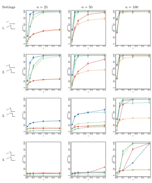
Sparsity patterns We study six different sparsity patterns as summarized in Table1. The first two are meant to validate type I error control. The last four allow us to compare the performances of the various test statistics, collections and calibrations under different sparsity levels and proportions of shared coeffi-cients. In all cases, the choices of sparsity parametersηandη2lead to strong to very strong levels of sparsity. The last column of Table1 illustrates the signal sparsity patterns ofβ(1) andβ(2) associated with each scenario. In scenarios 1 and 2, sample-specific signals share little, if not none, non zero coefficient. In scenarios 3 and 4, sample-specific coefficients show some overlap. Scenario 4 is the most difficult one since the number of sample-2-specific coefficients is much smaller than the number of common non zero coefficients: the sparsity of the difference betweenβ(1)andβ(2) is much smaller than the global sparsity ofβ(2). This explains why the illustration in the last column might be misleading: the two patterns are not equal but do actually differ by only one covariate.
Beyond those six varying sparsity patterns, we consider three different cor-relation structures Σ(1) and Σ(2) for the generation of the design matrix. In all three cases, we assume that Σ(1) = Σ(2) = Σ. On top of the basic orthogonal matrix Σ(1) = Σ(2) = I
p, we investigate two randomly generated correlation
structures.
Power decay correlation structure First, we consider a power decay correlation structure such that Σi,j = ρ|i−j|. Since the sparsity pattern of β(1) and β(2)
is linked to the order of the covariates, we randomly permute at each run the columns and rows of Σ in order to make sure that the correlation structure is independent from the sparsity pattern.
Gaussian graphical model structure Second, we simulate correlation structures with theRpackageGGMselect. The functionsimulateGraphgenerates covari-ance matrices corresponding to Gaussian graphical model structure made of


![Fig 6. Graphs of conditional dependencies among the 26 genes selected by [23] on patients with pathologic complete response or residual disease with medium regularization as presented in Figure 3 of [1].](https://thumb-us.123doks.com/thumbv2/123dok_us/653974.2578868/35.918.203.633.707.930/conditional-dependencies-selected-patients-pathologic-complete-regularization-presented.webp)