Mobile hyperspectral imaging for structural damage detection

(1)

MOBILE HYPERSPECTRAL IMAGING FOR STRUCTURAL DAMAGE DETECTION

A THESIS IN Civil Engineering

Presented to the Faculty of the University Of Missouri-Kansas City in partial fulfillment of

The requirement for the degree

MASTERS OF SCIENCE

by

SAMEER ARYAL

B.E. Tribhuwan University, Kathmandu, Nepal, 2016

Kansas City, Missouri 2020

(2)

(3)

iii

MOBILE HYPERSPECTRAL IMAGING FOR STRUCTURAL DAMAGE DETECTION

Sameer Aryal, Candidate for the Master of Science Degree University of Missouri -Kansas City, 2020

ABSTRACT

Numerous optical-imaging and machine-vision based inspection methods are found that aim to replace visual and human-based inspection with an automated or a highly efficient procedure. However, these machine-vision systems have not been entirely endorsed by civil engineers towards deploying these techniques in practice, partially due to their poor performance in object detection when structural cracks coexist with other complex scenes. A mobile hyperspectral imaging system is developed in this work, which captures hundreds of spectral reflectance values at a pixel in the visible and near-infrared (VNIR) portion of the electromagnetic spectrum bands. To prove its potential in

discriminating complex objects, a machine learning methodology is developed with classification models that are characterized by four different feature extraction processes. Experimental validation with quantitative measures proves that hyperspectral pixels, when used conjunctly with dimensionality reduction, possess outstanding potential in recognizing eight different structural surface objects including cracks for concrete and asphalt surfaces, and outperform the gray-values that characterize the texture/shape of the objects. The authors envision the advent of computational hyperspectral imaging for automating structural damage inspection, especially when dealing with complex structural scenes in practice.

(4)

iv

APPROVAL PAGE

The faculty listed below, appointed by the Dean of the School of Computing and

Engineering have examined the thesis titled “Mobile Hyperspectral Imaging for Structural Damage Detection”, presented by Sameer Aryal, candidate of the Masters of Science degree, and certify that in their opinion it is worthy of acceptance.

Supervisor Committee

ZhiQiang Chen, Ph.D., Committee Chair Department of Civil and Mechanical Engineering

John Kevern, Ph.D., P.E., LEED AP Department of Civil and Mechanical Engineering

Ceki Halmen, Ph.D., P.E.

(5)

v

LIST OF ILLUSTRATIONS

Figure Page

1. A hyperspectral image data ...11

2. Reflectance plot for asphalt, color, concrete, crack, dry vegetation, oil, green vegetation, and water respectively with 20 random pixels ...14

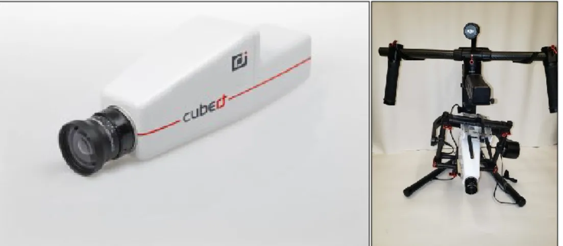
3. Cubert hyperspectral camera and assembly system at UMKC ...15

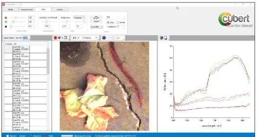
4. Cubert pilot application to visualize and extract the hyperspectral data ...17

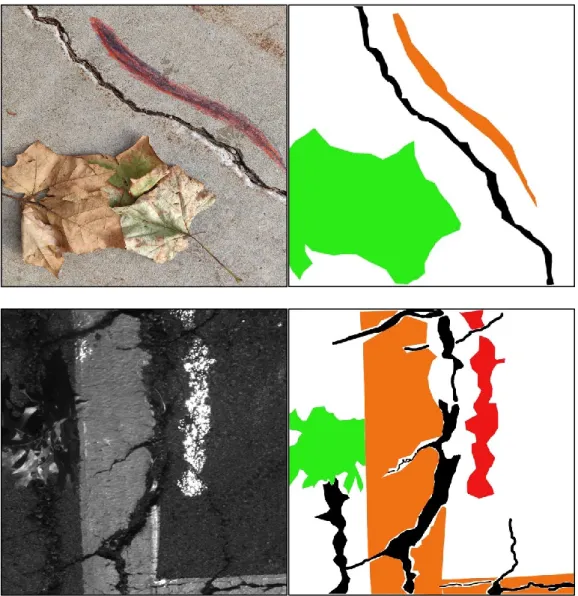
5. Images of concrete and asphalt surface with feature and their respective ground truth images ...19

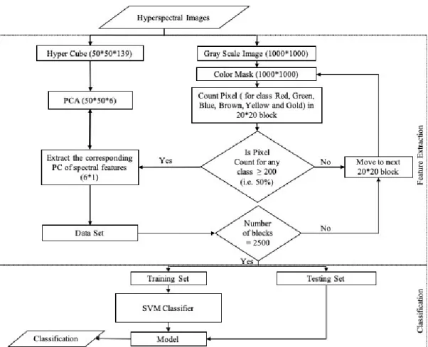
6. Dimensionality reduction and classification approach for the hyperspectral image . ... 20

7. HOG feature extraction and classification approach. ...21

8. A combined PCA and HOG feature extraction and classification approach ...21

9. Distribution of the first, second and third principal components of concrete, asphalt, color, crack, dry vegetation, green vegetation, water, oil dataset ...26

10.The first and second principal component distribution plot the dataset ...27

11.Block diagram for feature extraction with HOG feature descriptors ...28

12.Decision boundary and margin of SVM classifier. ... 34

13.ROC curve for model M2(HYP_PCA) and M3(GL_HOG) (Case-I). ...45

14.Precision-Recall curve for M2(HYP_PCA) and M3(GL_HOG) (Case-I) ...46

15.ROC curves for model M2(HYP_PCA) and M3(GL_HOG) (Case-II) ...49

16. Precision-Recall curves for model M2(HYP_PCA) and M3(GL_HOG) (Case-II) ...50

(8)

viii

18.Precision-Recall curve for model M2(HYP_PCA) and M3(GL_HOG) (Case-III) ...52 19.Training and testing time comparison plot ...57

(9)

ix

LIST OF TABLES

Table Page

1. Performance summary of model M1(HYP) ...42

2. Performance summary of model M2(HYP_PCA) ...43

3. Confusion matrix for model M2(HYP_PCA) (Test-I)...46

4. Confusion matrix for model M3(GL_HOG) (Test-I) ...47

5. Performance summary for model M3(GL_HOG) ...48

6. Confusion matrix for model M2(HYP_PCA) (Test-II) ...50

7. Confusion matrix for model M3(GL_HOG) (Test-II) ...51

8. Confusion matrix for model M2(HYP_PCA) (Test-III) ...53

9. Confusion matrix for model M3(GL_HOG) (Test-III) ...53

(10)

x

ACKNOWLEDGMENTS

First and foremost, I would like to take this opportunity to express my deepest gratitude and thanks to my advisor, Dr. ZhiQiang Chen, for his countless effort in guiding me through studies and work, his patience with my learning and providing me with an excellent atmosphere for research. This thesis would not have been complete without his attitude and diligent effort which not only influences the content of this thesis but also the language in which it has been conveyed. I am sure it would have not been possible

without his help.

Also, I would like to thank my colleague at the University of Missouri Kansas City: Prativa Sharma, Shimin Tang, and Mostafa Badroddin for their effortless help, valuable advice, and discussion. We had great and unforgettable times during all these years.

Last but not least, I am so thankful to my family whom they have been a continuous source of encouragement and supports in all directions during my life.

(11)

1

CHAPTER 1. INTRODUCTION

Civil engineering structures are complexly planned systems that are vital for a society’s prosperity and quality of life in general. Ensuring the reputation, civil engineering structures have grown its dynamic demand around the globe over the past few decades. Apparently in the United States, there are over 610,000 bridges, 5,500,000 commercial buildings, 160,000 miles of railroad tracks, 4,000,000 miles of roads, 84,000 dams, 19,000 airports and 400,000 miles of electric transmission lines providing services to the population (ASCE, 2017). These structures are built and maintained to support the daily routine load as well as the additional unexpected loads and the unavoidable severe environmental conditions. For critical infrastructure systems, mandatory inspection practices and standards exist for adoption by stakeholders to ensure the serviceability and safety of the structure. One of them is for a comprehensive diagnostics and prognostics of serviceability of the national infrastructures, American Society of Civil Engineers

(ASCE) has developed the ‘Infrastructure Report Card’ which grades the infrastructures as A- Exceptional, Fit for the Future; B- Good, Adequate for now; C- Mediocre, Requires Attention; D- Poor, At-Risk; and F- Critical Unfit for purpose.

Civil engineering structure inspection is more on the overall and general

conditions, as can be directly observed or measured. The task of inspection for evaluation of civil engineering structure status has become increasingly challenging due to age, scale, and magnitude of structures. Different civil engineering inspection techniques are in practice to assist visual inspection. Exclusively these practices are to stipulate valuable information for structural assessment and decision support for maintenance through relevant measures of structural responses. These technologies can be generally

(12)

2

utilizing advanced sensing technologies (microwaves, thermal and ultrasonic) (Cawley, 2018), most of which aim to detect subsurface damage. The second methodology includes various structural health monitoring (SHM) methods, which aim to monitor the dynamic responses and identify the intrinsic parameters or changes in structure. Most NDT techniques have become a growing field that has attracted a considerable amount of research efforts. Given these technology-based inspections or monitoring methods, the reality is that, at least for transportation structures that are managed by the department of transportation (DOT) agencies across most of the states in the US, manual or visual inspection is considered the mainstream approach. Sadly, despite the critical roles of these structures in public safety and economy, human-based visual inspection is common and consistent in quantitative evaluation and accessibility (Graybeal, Phares, Rolander, Moore, & Washer, 2002). Visual inspection is widely used mostly due to the expensive approach of the NDT techniques which demands a significant operational cost including training and deployment of manpower and technology in the field. Due to the low-cost and ubiquitous availability of optical imaging sensors or commonly speaking, digital cameras, it is of no surprise that optical imaging has become a widely adopted equipment for structural inspection, wherein besides visual inspection, digital images are recorded for records or for post-inspection analysis (M. J. Olsen et al., 2016). Among many methods for surveillance with the digital camera, one of them includes placing cameras at different critical locations around the structure and constantly monitoring the deformation and deterioration. This method covers only a small section of the structure and records mostly the textural information which alone is never enough for a complete structural assessment. To overcome the limitation, an alternative system is implemented which involves gathering images and registering the conditions of the surface by a skilled

(13)

3

technician traveling along the surface while taking pictures. After the structural surface images are captured, skilled technicians analyses each image and determine the existence of any distress and classify damage type based on visual descriptions. This process usually is time-consuming and requires a huge effort to analyze the full set of acquired images. Hence there arises a need for a rapid data acquisition and classification platform to collect, process and classify the structural surfaces in interest. These techniques have emerged with an essential goal of safeguarding the operational safety of structures, through deploying various types of sensors, monitoring diversified physical quantities, assessing structural condition and performance, and instructing routine inspection and maintenance. Subsequently, this has motivated the movement of developing machine vision techniques to aid or event to automate engineering inspection of civil structures.

Machine vision is a technical field that concerns the development of digital imaging methods and the use of image processing or computer vision algorithms for the extraction of useful information from images (Morris, 2004). With the advent of early digital cameras, researchers in the last eighties and nighties used simple digital filters, including various edge detection methods, for realizing image-based structural damage detection (Cheng & Miyojim, 1998; Ritchie, 1987; Ritchie Stephen, 1990). To further automate the process of image capturing, researchers further strive to develop other imaging methods that are expected to mitigate the human cost of professional inspectors. These novel methods include ground vehicle-based imaging, aerial vehicle-based

imaging, and crowdsourcing based imaging [e.g., (Isawa et al., 2005; Kim, Sim, & Cho, 2015; Lattanzi & Miller, 2013; Tung, Hwang, & Wu, 2002; C. Zhang & Elaksher, 2012) (Ozer, Feng, & Feng, 2015)]. For example, Ho et al. (2013) developed a system with three cameras attached to a cable climbing robot to detect surface damage (Ho, Kim,

(14)

4

Park, & Lee, 2013). Yeum and Dyke (2015) proposed an unmanned aerial vehicle (UAV) for remote imaging and image-based detection (Yeum & Dyke, 2015). In Chen et al. (2015), a mobile-cloud infrastructure enabled approach was proposed that exploits collaborative mobile and cloud computing to harness crowdsourcing-based structural inspection (Chen, Chen, Shen, & Lee, 2015).

Unlike, regular digital imaging process, the author develops a mobile

hyperspectral imaging (HSI) system for both ground and aerial vehicle-based remote sensing. With this HSI system and preliminary observation (e.g., by plotting spectral profiles for different structural surface objects), it is hypothesized that structural damage (e.g., cracks) and other complex artifacts can be effectively detected on structural

surfaces. Furthermore, this HSI system equipped with a machine learning approach can outperform the performance of regular imaging methods with a high spatial resolution (i.e., those based on panchromatic or true-color imaging). The essential contribution of this thesis is the proven effectiveness of mobile HSI for structural surface damage detection with complex scenes. Different from any existing image-based structural damage detection method, in this study, the proposed framework deals with the detection problem with much semantically rich structural-surface materials and objects, including concrete, asphalt, crack, dry vegetation, green vegetation, water, oil, and artificial markings, which are dealt with in the literature of image-based damage detection but commonly found in engineered structures in service. Another significant contribution is the semantically labeled dataset resulting from this research, which provides an

unprecedented basis for research in hyperspectral machine vision and engineering inspection automation.

(15)

5

Literature Survey

With the abundance of these optical imaging platforms, one promising fact is the ease of obtaining imagery structural-damage databases. Other than early vision methods, these databases enable the adoption of a machine learning paradigm for image-based structural damage detection. Most of the techniques in these early efforts used either of one of the gradient-based edge detection (Shrivakshan & Chandrasekar, 2012), Hugh transformed based line detection methods (Song & Lyu, 2005), wavelet-based processing method (Abdel-Qader, Abudayyeh, & Kelly Michael, 2003; M. Olsen, Chen, Hutchinson, & Kuester, 2012), image binarization method (Cheng, Shi, & Glazier, 2003; Oliveira & Correia, 2009), percolation method (Tomoyuki, Shingo, & Shuji, 2008) or, shape-based modeling method (Chen & Hutchinson, 2010; Huo, Yang, Li, & Zhou, 2017). Some studies explored the methodology for automated surface cracks monitoring and

assessment of concrete surface, based on adaptive digital image processing Adhikari et al. (2014) and infrared thermography Sakagami (2015) whereas some other incorporated the displacement and strain measurement with digital imaging for crack defragmentation (Adhikari, Bagchi, & Moselhi, 2014; Sakagami, 2015; Valença, Dias-da-Costa,

Gonçalves, Júlio, & Araújo, 2014). Many different integration approaches of two or more sensors were explored and broadened to be used in more specific application categories. Vaghefi et al. (2015) developed a combined nondestructive imaging technology on the bridge deck to yield both surface and subsurface indicators of the condition (Vaghefi, Ahlborn Theresa, Harris Devin, & Brooks Colin, 2015). Stabile et al. (2012) used a suite of microwaves radar interferometer and a thermal camera to monitor the dynamic

displacement of bridges (Stabile et al., 2012). Waldbjorn et al. (2014) obtained the feedback signals i.e. strain and displacement by fiber Bragg grating and digital image

(16)

6

correlation aligned to monitor the mandrel position by measuring the rigid body displacement based on a multivariate least-squares algorithm (Waldbjørn et al., 2014). Other than early vision methods, these databases enable the adoption of a machine learning paradigm for image-based structural damage detection. As of today, many machine learning methods are found, which feature the use of supervised or

non-supervised classifiers (Chen, Derakhshani, Halmen, & Kevern, 2011; Gavilán et al., 2011; Kaseko & Ritchie, 1993; Liu, Suandi, Ohashi, & Ejima, 2002; Prasanna et al., 2014; Zakeri, Nejad, & Fahimifar, 2017). In recent years, coincident with the advances in artificial intelligence (AI), and particularly the development of deep learning techniques, many have heralded the era of AI-enabled structural inspection. To this end, a simple search through Google Scholar, using the combined keywords of “Crack Detection”, “Convolutional Neural Network” (CNN), and “Image” returns more than 700 articles within the period of January 2016 to October 2019. Notably, Zhang et al. firstly used a CNN model as a feature extractor then fed the features into a classification model for the detection of cracks in images (L. Zhang, Yang, Zhang, & Zhu, 2016). Such a CNN-based machine learning approach is then adopted in many other similar efforts [e.g., (Alipour, Harris, & Miller, 2019; Cha, Choi, & Büyüköztürk, 2017; Ni, Zhang, & Chen, 2019)]. One may expect that by duly considering the advances in these AI-enabled image-based damage detection methods and the lowering cost of mobile or edge computing devices, the notion of an autonomous structural inspection may become a reality. The authors in this paper argue that if a fundamental fact is not acknowledged, the pace of automation would ultimately be hindered. This fact is the complexity of structural scenes captured in digital images. In the case of concrete structures, the scenes in images are often a mixture of structural materials, possible damage, and other artifacts, such as artificial marking,

(17)

7

vegetation, moisture, oil spill, discoloring, and uneven illumination (Chen & Hutchinson, 2010). This implies that any image-based machine learning method or an end-to-end deep learning method may encounter the infamous issue of generalization. In other words, if such an autonomous image-based system is deployed in the field, its core detection component (i.e., a classification model) even trained based on a relatively large dataset with complex scenes, can over-fit the training data but cannot generalize to an arbitrary scene that is more complex than the data used for training.

To resolve this challenge, one obvious solution is to continue developing much larger dataset given the power of deep learning with an architecture that can potentially accommodate any scale of data sizes and any complexity in field scenes, when regular images (i.e., true-color images with red, green, and blue bands or RGB images) are continuously used. However, this inevitably triggers the issue of labeling big data (e.g., pixel-wise labeling of cracks and other artifacts), which is expensive and time-consuming (Roh, Heo, & Whang, 2019). Another approach is to resort to transfer learning and use small data sets enhanced by effective data augmentation technique to obtain the notion of learning from small data using DL models. A recent effort of such is reported (Shimin Tang & Chen, 2017), which develops a crack pixels-based data augmentation technique for fine-tuning of DL models. Regardless of the potential success in these solutions, it is asserted that with the use of RGB images, the outcomes of developing these methods can only asymptotically match the intelligence of trained inspectors, though possibly with much higher efficiency than human inspectors. In other words, there is a performance ‘ceiling’ that tops the capacity of regular RGB images unless that machine intelligence supersedes human beings.

(18)

8

An alternative solution is to break out the normal of matching human vision. An emerging technology for structural inspection is hyperspectral imaging (HSI). In a hyperspectral image, a pixel contains tens to thousands of digital values at different spectral bands in the visible and near-infrared (VNIR) portion of the electromagnetic spectrum bands, at which each digital value represents either the reflectance or

transmittance property of a material at one band. Such a high-dimensional spectral profile hence is not directly visible to human eyes that respond, roughly speaking, only to three discrete bands (namely, red, green, and blue)(Kaiser & Boynton, 1996). Scientific knowledge in hyperspectral imaging and analysis is well archived and is, in general, termed hyperspectral spectroscopy (Siesler, Ozaki, Kawata, & Heise, 2008). In the context of image-based structural damage detection, it is stated that HSI provides a significant possibility of detecting and identifying the presence of either structural damage or noisy artifacts at the material level.

In this work, the authors develop a mobile hyperspectral imaging (HSI) system for both ground and aerial vehicle-based remote sensing. With this HSI system and

preliminary observation (e.g., by plotting spectral profiles for different structural surface objects), it is hypothesized that structural damage (e.g., cracks) and other complex artifacts can be effectively detected on structural surfaces. Furthermore, this HSI system equipped with a machine learning approach can outperform the performance of regular imaging methods with a high spatial resolution (i.e., those based on panchromatic or true-color imaging). Different from any existing image-based structural damage detection method, in this study, the proposed framework deals with the detection problem with much semantically rich structural-surface materials and objects, including concrete, asphalt, crack, dry vegetation, green vegetation, water, oil, and artificial markings, which

(19)

9

are dealt with in the literature of image-based damage detection but commonly found in engineered structures in service. Another significant contribution is the semantically labeled dataset resulting from this research, which provides an unprecedented basis for research in hyperspectral machine vision and engineering inspection automation.

Literature Survey Summary

To summarize the literature review, certain areas are yet to be explored and new improved systems are yet to be developed for the damage detection in civil engineering structures. While there have been researches focused on the detection of cracks,

defragmentation and damage assessment on the surface using images and videos but these results lack when considering the complex and realistic scenes. This review shows that the implementation of a computer vision-based method for non-destructive testing and its potential to provide more valuable information for the visual inspection and structural condition assessments through integration with other sensing techniques as well as presents some critical limitations and challenges of the system. Most of the current research is conducted through the images captured in a controlled environment. The quality of the image captured by the vision device will be significantly affected by the surrounding environment condition such as mixer of the contrast from other similar materials, light variation, presence of oil or water on the surface and artificial marks on the surface which are very common on the structural surface. Along with image quality limitation, the majority of the current literature focuses on binary classifications using simple machine learning techniques or threshold-based heuristics. However, multiclass classification has not yet been explored for different classes of damages found on the civil engineering structures.

(20)

10

In the following, first, the concept of HSI is briefly introduced, and a mobile HSI system is described. In the next, the machine learning methodology is introduced with a focus on proving the concept of HSI-based detection and its competitive performance. Performance evaluation and discussion are further conducted with four classification models, followed by a summary of conclusions and vision at the end.

(21)

11

CHAPTER 2. HYPERSPECTRAL IMAGE

When a beam of white light is dispersed by passing through a prism, a continuous range of colors, the so-called color the spectrum is formed. All object gives off

electromagnetic radiation and it has been known that different materials emit, reflect and absorb a different proportion of lights and this proportion is the function of the frequency of the light wave (Richards & Jia, 1999). Since the color spectrum visible to the human eye is only a small region of the much wider electromagnetic spectrum thereby detecting and analyzing the energy emitted or reflected, an enormous amount of information about the material into consideration can be obtained. This specific property of the physical object is called reflectance. The reflectance of an object varies at different wavelength producing a unique electromagnetic spectrum profile for each object.

The imaging spectroscopy is defined as “the simultaneous acquisition of the measurement, processing, and analysis of images in many narrow, contiguous spectral bands” (Goetz, Vane, Solomon, & Rock, 1985). The concept of HSI originated in the 1980s when Goetz and his colleagues at the Jet Propulsion Laboratory (JPL) began developing the seminal instrument of the Airborne Visible/Infrared Imaging Spectrometer (AVIRIS) (R. O. Green et al., 1998; Plaza et al., 2009). Different from gray-level or RGB images, in a hyperspectral image, a hyperspectral pixel consists of a large number of intensity values sampled at different narrow spectral bands that represent the contiguous spectral curve at the pixel. A Hyperspectral image, in general, can be assumed as a 3D data cube structure, where a 2-D spatial-domain resides over a 1-D spectral-domain. One may view each hyperspectral data cube as a stack of spatially registered 2D images at different wavelengths (bands). Each pixel is a 1-D vector, corresponds to the reflectance energy spectrum within its field of view (FOV) (Richards & Jia, 1999). Figure1 shows

(22)

12

full three-dimensional hyperspectral (two spatial dimensions plus one wavelength dimension) data cube.

Figure1. A hyperspectral image data (Bodkin et al., 2009a)

For hyperspectral images obtained by advanced hyperspectral cameras, detailed spectral information and fine spatial resolution enable an analysis of both materials and structures of the object in a scene. Therefore, it is necessary to develop new techniques to exploit these underlying spatial and spectral information in hyperspectral images, thus advancing the limitation of human vision, computer vision, and remote sensing. Some attempts have been made in both computer vision and remote sensing over time but still, there has been a huge gap between hyperspectral imaging and material classification application due to lack of effective spectral-spatial feature extraction method as well as due to lack of enough data and robust classification method.

Hyperspectral Imaging Technology

As advances in HSI and especially sensors that are not for orbital or airborne platforms, the acquisition of hyperspectral data cubes can be realized with other

(23)

13

mechanisms (spectral scanning and spatial-spectral scanning) are developed for HSI applications in medical and biological sciences (Lu & Fei, 2014). It is noted that towards producing a hyperspectral cube, these three scanning techniques require complex post-processing steps to achieve the end product, a data cube. The fourth mechanism is the non-scanning or ‘snapshot’ imaging (Johnson, Wilson, Bearman, & Backlund, 2004). The snapshot imaging, different from other, acquires spectral pixels in a 2-D field-of-view simultaneously, without the requirement of trajectory flights or using any moving parts in the imager. Therefore, this ‘snapshot’ mechanism is also referred to as real-time HSI by researchers (Bodkin et al., 2009b). This HSI mechanism can achieve much higher frame rates and higher signal-to-noise ratios and can provide hyperspectral cubes immediately after every action of capturing as in a regular digital camera. Due to this property, real-time or ‘snapshot’ HSI opens up significant opportunities for its use in portable, mobile, or low-altitude remote sensing.

Hyperspectral Image Computing

Given a hyperspectral cube, one can denote it as h(x, y, s) acquired from several spectral bands (i.e., for visible bands s ∈ [400, 600] nm; and visible to near-infrared, s ∈ [400, 1,000] nm). At a select location of (x, y), therefore, h(x, y, s) represents a spectral profile when plotted against the variable spectral s. In the remote-sensing context (not in a medical or biological context), namely, the data cube is acquired in the air, and the

measurement at the sensor is the upwelling radiance. In general, it is the reflectance property of a material at the ground that nominally does not vary with solar illumination or atmospheric disturbance. Therefore, the acquired spectral profile reflects the

characteristics or signatures of the material. Therefore, a raw radiance data cube needs to be corrected to generate a reflectance cube, considering the environmental lighting and

(24)

14

the atmospheric distortion. This process is called atmospheric correction (Adler-Golden et al., 1998). Figure 2. Below represents the plot for the reflectance plot for each material class we have opted to work within this thesis work.

(25)

15

Figure 2. Reflectance plot for asphalt, color, concrete, crack, dry vegetation, oil, green vegetation, and water respectively with 20 random pixels.

Camera Calibration

The raw spectral image collected using the hyperspectral imaging system is

detector signal intensity. To calibrate the raw intensity images into reflectance, calibration of the camera is performed with the help of a black and white reflectance image. This process corrects the significant signal vibrations, which are caused by non-uniformity of the illumination and the focal plane array of the camera, known as pattern noise (Nouri, Lucas, & Treuillet, 2013). Natively, the imager captures radiance images, and with the internal processing and a proper calibration procedure, the camera can output reflectance images directly. To do so, a reflectance calibration process starts with the use of a

standard white reference board, achieving a data cube for the standard whiteboard (denoted as hW). Second, a ‘perfect dark’ cube is obtained (by simply covering the lens tightly with a black cap), denoted as hB. The relative reflectance image, h, is calculated given a radiance cube hR,

ℎ = ℎ𝑅 − ℎ𝑤

ℎ𝑤−ℎ𝐵 (1)

Following Eq. (1), a reflectance image can be produced by the camera directly or can be post-processed from the produced radiance image.

(26)

16

CHAPTER 3. PREPROCESSING

This section describes the data collection process with the developed application, specifications of the hardware, data format, and information about the environmental setup are also described in detail. For the data acquisition and processing, the most important components are the camera and its specification that determines the resulting quality of the collected data.

Imaging System

A mobile HSI system for ground-level and low-altitude remote sensing is developed by the authors. The imaging system consists of a Cubert S185 FireflEYE snapshot camera that combines the precision of hyperspectral camera with the ease of snapshot camera, accurately capturing data over the whole field of view, and a mini-PC server for onboard computing and data communication (Cubert Gmbh, 2018). For ground-based imaging, the system is mounted to a DJI gimbal that provides two 15-W and 1580 mAh batteries for powering both the imaging payload and the operation of the gimbal. Figure 3 shows the gimbaled imaging system, which is ready for hand-held or other ground-based HSI. To enable low-altitude remote sensing, an unmanned aerial vehicle (UAV) is used, and the gimbaled system can be easily installed to the UAV for remote sensing.

(27)

17

This device has a wavelength range of 450nm to 950nm with a spectral resolution of 8nm capturing 139 channels and a pan resolution of 2500 spectral per cube providing a complete hyperspectral cube with a global shutter in 1/1000 of a second, without the need of IMU. As per the manufacturer, the wavelength accuracy at 532nm and 808nm are respectively ±2.5nm and ±4.5nm. One unique feature of the Cubert HSI system is its dual acquisition of hyperspectral cubes and a companion image, a gray-level intensity image. The gray-level image has an identical field of view as the hyperspectral cube but has a much higher spatial resolution, which has a size of 1,000 × 1,000. Denoting this gray image as g(u, v), one can ‘fuse’ g(u, v) and h(x, y, s) to achieve a hyperspectral cube with a higher resolution, and at its peak, one can obtain a cube with the size of 1,000 × 1,000 × 139. This process is called pan-sharpening, and to obtain smooth sharpening effects, many algorithms exist (Loncan et al., 2015). Nonetheless, it is noted that pan-sharpening, which can provide visually appealing hyperspectral images (if visualized in terms of pseudo-color images), does not provide new information compared to the original low-resolution hyperspectral cube and the high-low-resolution gray image. Therefore, in this paper, the low-resolution data cubes are directly used towards the goal of pattern classification-based object detection.

The Cube-Pilot is the official graphical user interface (GUI) to the Cubert Hyperspectral cameras making it possible to calibrate the camera before taking any pictures and aiding in the process of image capturing. A window of the Cube-pilot application is shown in Figure 4.

(28)

18

Figure 4. Cube pilot application to visualize and extract the hyperspectral data. Semantic Labelling

With the mobile HSI system (Figure. 3), a total of 68 instances of hyperspectral images (and their companion gray-level images) were captured in the field. Among these images, 43 images come from concrete surfaces and 25 images from asphalt surfaces. To create scene complexity, artificial markings, oil, water, green and dry vegetation were added in 34 of concrete images and 16 of asphalt images that have hairline or apparent cracks. Of the remaining 18 images, 9 images were taken from the surfaces of concrete and asphalt pavements without cracks and any of the other artifacts, respectively.

To create a supervised learning-ready dataset, manual and semantic labeling is carried out. Semantic labeling is the process of labeling each pixel in an image with a corresponding class label. In this work, an image-segmentation (or image parsing) based labeling approach is considered in which clustered segment with pixels belong to the same class is delineated in the image domain and rendered with a select color. The image of labeling is based on the gray-level image that accompanies a hyperspectral cube. In this work, this process was conducted by using an open-source image processing program, GIMP (Kimball & Mattis, 2019). As shown in Figure 5, during the labeling

(29)

19

process, a total of six different classes, including cracking, green vegetation, dry

vegetation, water, oil, and artificial marking, are assigned with the color of black, green, brown, blue, red, and yellow, respectively. It is noted that in this effort, the background materials (concrete and asphalt) are not classified in these complex-scene images as well as in the plain (concrete/asphalt) images. Figure 5 shows two samples of the original gray-level images and the resulting color-rendered mask images for a concrete surface and an asphalt surface, respectively.

Figure 5. Images of concrete and asphalt surface with features and their respective ground truth images

(30)

20

CHAPTER 4. METHODOLOGY

This section describes the proposed architecture and methodology followed in this thesis. Four machine learning algorithms based on the traditional machine-learning paradigm (namely, manually tuned feature extraction and select classification are employed) are designed in this work. With these algorithms, the specific objectives are two-fold:

1. Hyperspectral data can improve the accuracy of detection compared to gray-level images. 2. Dimensionality reduction can further improve the accuracy and robustness compared

against the case without dimensionality reduction.

Depending on the feature extraction methods, the following models are obtained. The list below summarizes these four models with abridged notations and their primary testing goals.

1. Model-1 or M1: feature extraction based on hyperspectral pixels with spectral values directly used as feature vectors. Namely, h(x, y, s) at (x, y) is directly used as a feature vector, where 𝑠 ∈ {1,2, … , 139}. To reflect this characteristic, an abridged notation M1(HYP) is used, where HYP represents the feature extraction process.

2. Model-2 or M2: feature extraction based on hyperspectral pixels with spectral values subject to a linear PCA as an additional feature selection step to reduce the dimensionality. Namely, the profile of h(x, y, s) at (x, y) is reduced to six dimensions only and becomes h’(x, y, k), where 𝑘 ∈ {1,2, 3, . . ,6}. For this model, M2(HYP_PCA) is used for simplicity. The flowchart for model

3. Model-3 or M3: feature extraction based on the companion gray-level images, g(u, v),

where the feature vectors at a 20 × 20 neighborhood in g(u, v) maps to the hyperspectral pixel at (x, y). To extract the gray-level features within a sliding 20×20 neighborhood in

(31)

21

g(u, v), the widely used gradient-based feature extractor, the histogram of gradients, or HOG, is considered and a variant of HOG is adopted in this paper. The resulting model is denoted by M3(GL_HOG.

4. Model-4 or M4: feature vectors based on the combined use of the feature vectors used in Model-2 and Model-3. Namely, by concatenating the two feature vectors, it fuses imagery information from both the hyperspectral pixel-based spectrum and the gray-value based spatial distribution. Hence, the notation of M4(GL_HOG+HYP_PCA) is used for simplicity, and GL_HOG+HYP_PCA represents the fourth feature extraction process in this paper.

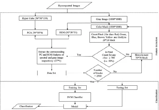
Figure 6. Dimensionality reduction and classification approach for the hyperspectral image.

(32)

22

Figure 7. HOG feature extraction and classification approach.

Figure 8. A combined PCA and HOG feature extraction and classification approach. With these models, the specific objectives towards proving the hypotheses are multi-fold:

Color Mask (1000*1000)

Is Pixel Count ≥ 200

(i.e. 50%)

Count Pixel ( for Red, Green, Blue, Brown, Yellow and Gold) in 20*20

block

Move to next 20*20 block Extract the corresponding

HOG feature (31*1) Data Set If the number of block is 2500

Training Set Testing Set

Model HOG (50*50*31) Pseudo-Color Image (1000*1000*3) Yes No No SVM Classifier Classification F ea tu re E xt ra ct io n C la ss if ic at io n Yes

(33)

23

 Objective-1: Evaluate the performance of the classification model of M1(HYP) hence to conclude if a hyperspectral pixel is effective in recognizing the underlying object types, including structural damage given a complex scene.

 Objective-2: Evaluate and compare the performance of M1(HYP) and M2(HYP_PCA), hence, to conclude if dimensionality reduction is effective in terms of improving the discrimination of different objects.

 Objective-3: Evaluate and compare the performance of M2(HYP_PCA) and M3(GL_HOG), hence, to conclude if hyperspectral pixels are more effective than high-resolution gray-level images towards identifying complex object types.

 Objective-4: Evaluate the performance of the classification model of M4(HYP_PCA, GL_HOG), hence, to conclude if, through simple data fusion, the combined hyperspectral and gray-level features provide more competitive detection performance. With the four models defined previously, they essentially differ in the use of different feature extraction processes based on the original hyperspectral data instance (a data cube and a companion gray-level image). With the colored mask images created as described above, it is denoted as m(u, v)sharing the same spatial domain as the underlying gray image g(u, v). For the sake of simplicity, based on the color coding for the mask images, the value of m(⋅) takes an integer value of 1, 2, …, 6 to indicate the underlying six different surface objects; in addition, the following notations are used to describe the resulting dataset:

𝒟 = { ℎ𝑛(𝑥, 𝑦, 𝑠), 𝑔𝑛(𝑢, 𝑣), 𝑚𝑛(𝑢, 𝑣)| 𝑛 = 1,2, … , 50} (2) To generate the machine-learning data for the models, the following feature extraction and treatment process is developed. Considering the spatial domains of a pair of h(x, y, s) and g(u, v), the following procedure is proposed:

(34)

24

1) Iterating with the location of (xi, yj) with i, j = 1, 2, …, 50, the spectral profile is stored in the vector of {h(xi, yj, s)| s ∈ [1, 139]}, and the gray-values in the corresponding gray image g(u, v) are confined in a neighborhood block of 𝒷 = {(u’, v’) | u’ ∈ [(xi -1)× 20 + 1, xi × 20], and v’∈[(yj -1)× 20 + 1, yj × 20]}. At this neighborhood of 𝒷, the gray-level image patch and the corresponding mask patch corresponding to the hyperspectral pixel at (x, y) are denoted as g(𝒷) and m(𝒷), respectively.

2) Given the mask patch m(𝒷), a simplified process is used to select the underlying class label for the hyperspectral pixel at (xi, yj). By counting the number of pixels belong to different object types within the neighborhood block 𝒷,

a. If a dominant class label exists, namely the number of pixels that belongs to a class is greater than 50% of the total pixels in the block (namely, 200 over 400 pixels), this class label is assigned to (xi, yj).

b. If no dominant class label exists, this pixel (xi, yj) and the corresponding neighborhood 𝒷 is skipped.

3) At a pixel with a dominant class label, and per the feature extraction method (HYP, HYP_PCA, and GL_HOG),

a. If HYP is used, {h(xi, yi, s)| s ∈ [1, 139]} is directly used as the feature vector with a dimension of 139 × 1.

b. If HYP_PCA is used, PCA is conducted over the vector {h(xi, yi, s)| s ∈ [1, 139]}, and the first 6PC scores are used to form a much low-dimensional 6× 1 feature vector.

c. If GL_HOG is used, the feature extraction is based on the gray-level patch g(𝒷) using the HOG-UoCTTI method, resulting in a 31× 1 feature vector.

(35)

25

d. If HYP_PCA + GL_HOG is fused, the two corresponding feature vectors are simply concatenated, resulting in a 37 × 1 feature vector.

4) By iterating this procedure over all the hyperspectral pixels for all the 50 instances of images which includes different types of features in consideration, the following classification data set is obtained for each of the feature extraction methods above.

𝒟𝐹𝐸𝐴 _{= { (𝒑}

𝒌, 𝑐𝑘)| 𝑘 = 1,2, … , 𝐾} (3) where the superscript FEA represents one of the feature extraction processes: HYP, HYP_PCA, GL_HOG, or HYP_PCA+GL_HOG. It is noted that by skipping many background pixels or pixels that do not have dominant labels in Step 2b, the resulting number of meaningful pixels (with dominant class labels) is 29546. Among them, 8132, 6495, 6273, and 5312 features are obtained for the class labels (ck’s) of water, oil, artificial marking and green vegetation, respectively. The number of features for cracks (concrete and asphalt cracks) is 2377. The dry vegetation features have the lowest number of 957.

With the data cubes and gray images for the plain concrete and asphalt surfaces (9 pairs each), 2601 features are arbitrarily extracted at each of feature extraction type but without using mask images each for the concrete or the asphalt labels. After adding these features into Eq. 3, the number of labeled features used in this paper, or K in Eq. 3, is 34748. As described above, given the lowest (957) and the largest (8132) number of features, a moderate imbalance indeed exists.

Principal Component Analysis (PCA)

Principal component analysis (PCA) is the most widely used linear-dimension method based on second-order statistics. PCA is also known as the Karhunen-Loeve transformation, singular value decomposition (SVD), empirical orthogonal function

(36)

26

(EOF), and Hotteling transformation. PCA is a mathematical procedure that facilitates the simplification of large data sets by transforming many correlated variables called

principal components. PCA finds a new set of orthogonal axes that have their origin at the data mean and are rotated to a new coordinate system so that the spectral variability is maximized. Resulting PC bands are linear combinations of the original spectral bands and are uncorrelated.

Given a hyperspectral profile at (x, y), or denoted as a set {h(x, y, s) | s ∈ [1, 2, …, 139]}, if treated as a feature vector, it gives rise to a 139×1 feature vector. As mentioned earlier, such high-dimensionality readily leads to poor performance when training a classification model (particularly when the training data is small, and the model itself cannot accommodate the high-dimensional space). Theoretically, assuming that an image had n pixels, measured at k spectral bands, the matrix characterizing the image is as follows. 𝐗 = [ 𝑥₁ ⋮ 𝑥𝑘 ] (4)

where x1… xk is a vector of n elements.

The first step in the PC procedure is generally the subtraction of the mean from each of the data dimesons. The mean spectrum vector represents the average brightness value of the image in each band and is defined by the expected value as follows:

𝑨 = 1 𝑁∑ 𝑥𝑗− [ 𝑥 ⋮ 𝑥_𝑘] 𝑁 𝑗=1 (5)

Where A is the mean spectrum vector, N is the total number of image pixels, and

xj is a vector representing the brightness of the jth pixel of the image. Therefore, the components of the mean spectrum vector A represent the average brightness of the image in each band. The mean shift is calculated by subtracting the mean of the data. The PC

(37)

27

analysis de-correlates the data mainly by rotating the original axes, and therefore, the mean shift does not change the attribute of the resulting PC images. The only difference is the addition of a constant value in each band. This makes the decorrelation more evident in subsequent stages but is not necessary.

The second step in the PC method is to calculate the covariance matrix, which is a square symmetric matrix, where the diagonal elements are variance and the off-diagonal elements are covariance. From a spectral imagery point of view, the variance represents the brightness of each band and the covariances represent the degree of brightness variation between bands in the image. Additionally, covariance that is large compared to the corresponding variance in a spectral pair indicates a high correlation between these bands while covariance close to zero indicates little correlation in these spectral pairs (Richards, 2013).

The covariance matrix is computed by the formula 𝑪 = 𝟏

𝒏−𝟏 (𝐗 − 𝐀)(𝑿 − 𝑨)

𝑻 ₍₆₎

Where A is the mean spectrum vector of the image and X is the vector

representing the brightness values of each pixel. The next step in the PCA analysis is the calculation of the eigenvectors and eigenvalues of the covariance matrix. The eigenvalues λ = {λ1 … λk}v of a k×k square matrix is its scalar roots and are given by the solution of the characteristic’s equation

|𝛴_𝑥− 𝜆𝑰| = 0 (7)

Where I is the identity matrix. The eigenvectors are closely related to the

eigenvalues and each one is associated with one eigenvalue. Their length is equal to one and they satisfy the equation

(38)

28

Where Vk is the eigenvector corresponding to the λk eigenvalue and its dimension is 1×k.

The eigenvectors are orthogonal to each other and provide us with information about the patterns of the data. The first eigenvector provides a line that approximates the regression line of the data- this axis is defined by maximizing the variance on this line. Therefore, the second eigenvector provides a line that is orthogonal to the first and contains the variance that is away from the primary vector. Then a regression plane can be defined for the data that maximizes the variance. When more than 3 variables are involved, the principles of maximizing the variance are the same but graphical representation is almost impossible.

The fourth step in the PC analysis is the determination is the components that can be ignored. An important property of the eigenvalue decomposition is that the total variance is equal to the sum of the eigenvalues of the covariance matrix, as each eigenvalue is the variance corresponding to the associated eigenvector. The PC process orders the new data space such that the bands are ordered by variance, from highest to lowest. The

eigenvector with the highest eigenvalue is the first principal component (PC) and accounted for most of the variation in an image. The second PC has the second larger variance being orthogonal to the first PC, and so on. Figure. 9 presents the variation of the three principal components for each class that are considered for training and testing the classifier.

(39)

29

Figure 9. Distribution of the first, second and third principal components of concrete,asphalt, color, crack, dry vegetation, green vegetation, water, and oil dataset. A transformed data set is created by using the eigenvectors from the diagonalization of the covariance or correlation matrix. After selecting the eigenvectors that should be retained, the following formula is applied:

(𝐹𝑖𝑛𝑎𝑙 𝐷𝑎𝑡𝑎 𝑆𝑒𝑡) = (𝐸𝑖𝑔𝑒𝑛𝑣𝑒𝑐𝑡𝑜𝑟𝑠 𝐴𝑑𝑗𝑢𝑠𝑡𝑒𝑑)′_{× (𝐷𝑎𝑡𝑎 𝐴𝑑𝑗𝑢𝑠𝑡𝑒𝑑)′} ₍₇₎ Where (Eigenvector Adjusted)’ is the matrix of eigenvectors transposed so that the eigenvectors are in the row with the first eigenvector on the top and (Data adjusted)’ is the matrix with the mean-corrected data transposed.

(40)

30

Figure 10. The first and second principal component plot of the dataset. Histogram of Oriented Gradient (HOG)

The Histogram of Oriented Gradient (HOG) feature descriptor aims to characterize the contextual texture or shape of objects in images through counting the occurrence of gradient orientations in a select block in an image or the whole image. It was first proven effective by Dalal and Triggs (2005) in their seminal effort for pedestrian detection in images (N. Dalal & Triggs, 2005); since then, HOG has been applied extensively for different objective detection tasks in the literature of machine vision. HOG differs from other scale-invariant or histogram-based descriptors in that its extraction is computed over a dense grid of uniformly spaced cells, and it uses overlapping local contrast normalization for improved performance. To this date, there are many variants of HOG descriptors for improving the robustness and accuracy; and a commonly used one is the HOG-UoCTTI as described in (Felzenszwalb, Girshick, McAllester, & Ramanan, 2010).

The basic idea behind HOG is; the appearances and shape of local objects within an image can be well described by the distribution of intensity gradients as the votes for

(41)

31

dominant edge directions. Such a feature descriptor can be obtained by first dividing the image into small contiguous regions of equal size called cells, and collecting a histogram of gradient directions for the pixels within such cells, and hence combining all these obtained histograms from each cell. To improve the detection accuracy against varied illumination and shadowing, local contrast normalization can be applied by computing a measure of the intensities across a larger region of an image, called a block, and using the resultant value to normalize all the cells within the block. Hence HOG consists of gamma and color normalization, gradient and orientation computation, cell histogram computation, normalization across blocks, and flattening into a feature vector. An overview of object detection with HOG is presented in figure 11.

Figure 11: Block diagram for feature extraction with HOG feature descriptors. The first step of HOG feature extraction is the computation of image gradients. The gradient tells how the image changes in the given direction. Gradient computation is done by applying the 1D centered, point discrete derivative most in both the horizontal and vertical direction while calculating gradient value for each pixel describing the relationship of neighboring pixel values according to the mask. Then, the magnitude and orientation at each pixel I(x, y) is calculated by

{

𝐺𝑚𝑎𝑔(𝑥, 𝑦) = √𝐺𝑥2(𝑥, 𝑦) + 𝐺𝑦2(𝑥, 𝑦) 𝜃(𝑥, 𝑦) = 𝑎𝑟𝑐𝑡𝑎𝑛 (𝐺𝑦(𝑥,𝑦)

𝐺𝑥(𝑥,𝑦)) + 𝜋 2⁄

(9)

Where Gx(x, y) and Gy(x, y) are the gradient values at each pixel in the horizontal and vertical direction, respectively.

In the next step, the histogram for each pixel region that is either rectangular or radial is created. The histogram bin is evenly expanded from 0º to 180º for unsigned and 0º

Input Image _{weighted vote into bins}Cell histograms: Block normalization Gamma and color normalization Gradient and Orientation Computation Features

(42)

32

to 360º for signed, so every histogram bin has a spread of 20º. Every pixel in the cell casts weighted voting into one of the 9 histogram bins which can either be the gradient magnitude itself or some function of the magnitude. The voting simply means increasing the frequency of the observed bin by the magnitude of the pixel.

Next, after generating cell histograms, to obtain the robustness against the various illumination and contrast, the gradient strengths must be locally normalized. This can be achieved by grouping the cells into lager pixels regions called bocks. Since the blocks overlap with the neighboring blocks, each block contributes its orientation distribution more than once. Since each scalar cell response contributes several components to the final descriptor vector, each normalized concerning a different block. Overlapping block adds redundant information that can improve the result significantly. There are four variants of the HOG block scheme: Rectangular HOG, Circular HOG, Bar HOG and Center-surround HOG (Navneet Dalal, 2006). (N. Dalal & Triggs, 2005) proposed and compared four different methods for block normalization. Let ʋ denote the non-normalized feature vector that collects all cell histograms from a given block ||ʋ||kdenotes its k-norm for k = 1, 2 and eps denote some small constant. Then the normalized scheme has the following forms:

𝐿2 − 𝑛𝑜𝑟𝑚: ʋ̂ = ʋ √||ʋ||22+𝑒𝑝𝑠2 (10) 𝐿1 − 𝑛𝑜𝑟𝑚: ʋ̂ = ʋ (||ʋ||₁+𝑒𝑝𝑠) (11) 𝐿1 − 𝑠𝑞𝑟𝑡: ʋ̂ = √_(||ʋ||ʋ 1+𝑒𝑝𝑠) (12) L2-Hys is computed by re-normalizing the clipped L2-norm. All the normalization scheme provides much better performance than the non-normalized case. Finally, the HOG feature is the vector containing the elements of the normalized cell histogram from all of the block regions.

(43)

33

In this effort, considering the resolution compatibility between the hyperspectral cube and the companion gray-level image, the feature extraction is conducted in a 20 × 20 sliding-neighborhood in a gray image. Within such a neighborhood four histograms of undirected gradients are averaged to obtain a no-dimensional histogram (i.e. binned per their orientation into 9 bins or no = 9) and a similar operation is performed for the directed gradient to obtain a 2no dimensional histogram (i.e. binned in accordance of their gradient into 18 bins). Along with both directed and undirected gradient, the HOG-UoCTTI also computes another four-dimensional texture-energy feature. The final descriptor is obtained by stacking the averaged directed histogram, averaged undirected histogram and four normalized factors of the undirected histogram. This leads to the final descriptor of size 4 + 3 × no (i.e., a 31 × 1 feature vector).

(44)

34

CHAPTER 5. MACHINE LEARNING APPROACH

Some of the first applications of machine learning to hyperspectral considered the task of classifying land cover, or terrain, into different classes, such as forest, water, agricultural land, and built uplands. Early approach tried to predict the class label ci at a pixel i from a vector Xi (Benediktsson, Swain, & Ersoy, 1990; Bischof, Schneider, &

Pinz, 1992; Paola & Schowengerdt, 1995), with the feature typically just taken to be the values at the different spectral bands at pixels i.

The Bayes’ classifier is one of the simplest and most popular approaches to terrain classification. The Bayes’ classifier makes explicit assumptions about the class

conditional distribution p (xiǀci = k) and the prior class probabilities P (ci = k) and uses Bayes’ rule to obtain the posterior class probabilities P (ci = kǀxi).Various other

simplifying assumptions lead to many popular classifiers. For example assuming that Σk is diagonal lead to the Naïve Bayes classifier for continuous inputs while assuming that P(ci = k) = 1/K lead to what is known in the remote sensing literature as the maximum likelihood classifier (Paola & Schowengerdt, 1995).

The main drawback of Bayes’ of the Bayes’ classifier is the need to explicitly specify the class-condition distribution p(xiǀci = k). Since the multivariate normal distribution is typically used for class-conditional distribution, only linear or quadratic decision boundaries can be learned by such a model. The neural network became a popular alternative to the Bayes’ classifier because they directly model p (xiǀci = k) as a differentiable function whose parameter is learned (Bischof et al., 1992; Lee, Weger, Sengupta, & Welch, 1990). This both sidesteps the need to specify p(xiǀci = k) and allows for richer, non-linear decision boundaries to be learned when at least one hidden layer of units with a non-linear activation function is used. Due to the ability to learn non-linear

(45)

35

decision boundaries, neural networks tend to give higher classification accuracies than various forms of Bayes’ classifier (Benediktsson et al., 1990; J. Zhang & Modestino, 1989). (Bischof et al., 1992) explored adding contextual information by using spectral values from a small patch at the pixel of interest as the input to a neural network, allowing it to learn some contextual features. Others aimed to improve classification accuracy by using hand-designed features that encoded local textural information. (Haralick,

Shanmugam, & Dinstein, 1973; Lee et al., 1990). (Haralick et al., 1973) introduced a popular set of features derived from gray-level values i, and j co-occur at distance d and angle θ.

Support Vector Machine

Discriminating between object classes with similar features, such as concrete, asphalt, vegetation, water, and oil requires some knowledge of spectral profile and context which in turn leads to much more complex decision boundaries than the ones required to discriminate forest and city areas from imagery. Due to the need to learn such highly nonlinear decision boundaries, applications of machine learning to high-resolution imagery have relied on more sophisticated classifiers. While the neural network can learn nonlinear decision boundaries and have been widely used in remote sensing applications, many researchers found them difficult to train due to the presence of local optima

(Benediktsson et al., 1990).

Support Vector Machine (SVM) has been employed in a wide range of real-world problems such as text categorization, handwritten digit recognition, tone recognition, object detection, image classification, regression problem and more colloquially learning from examples since purposed by Vapnik (Cortes & Vapnik, 1995). SVM has been proven to be a good candidate for the machine learning approach due to its high

(46)

36

generalization performance without the need for prior knowledge, even when the dimension of the input space is very high. Given a set of points which belongs to either one of two class, a linear SVM finds the hyperplane leaving the largest possible fraction of points of the same class on the same side while maximizing the distance of either class from the hyperplane. According to Vapnik, this hyperplane minimizes the risk of

misclassifying data from the test set. SVM has often been found to provide higher classification accuracies than other widely used pattern recognition techniques, such as maximum likelihood (Mondal, Kundu, Chandniha, Shukla, & Mishra, 2012) and the multilayer perceptron neural network classifier (Osowski, Siwek, & Markiewicz, 2004). Furthermore, SVM appears to be especially advantageous in the presence of

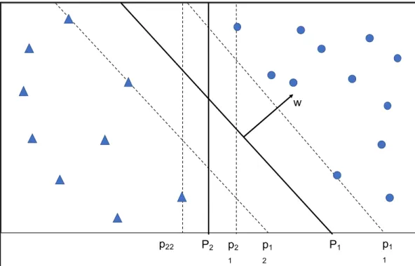
heterogeneous classes for which only a few training samples are available. In the context of hyperspectral image classification, some pioneering experimental investigations preliminary pointed out the effectiveness of SVM to analyze the hyperspectral data directly in the hyperdimensional feature space, without the need of any feature reduction techniques (J. A. Gualtieri & Chettri, 2000; J. Anthony Gualtieri & Cromp, 1999) In Figure 12, triangular data points belong to one of the classes and circular data points belong to another class. SVM tries to find a hyper-plane (P1 and P2) that separates the two classes. As shown in the figure there may be many hyperplanes that can separate the data but SVM chooses the best decision boundary based on the maximum margin

(47)

37

Figure 12. Decision boundary and margin of SVM classifier.

Each hyperplane (Pi) is associated with a pair of supporting hyper-plane (pi1 and pi2) that are parallel to the decision boundary (Pi) and pass through the nearest data point. The distance between these supporting planes is called margin. In the figure, even though both the hyperplane (P1 and P2) divide the data points, P1 has a bigger margin and tends to perform better for the classification of unknown samples than P2. Hence bigger the

margin is, less the generalization error for the classification of unknown samples is. Therefore, in the case of the above figure hyperplane P1 is preferred over hyperplane P2. For a linear SVM, the equation for the decision boundary is

𝒘 ∙ 𝒙 + 𝑏 = 0 (13)

Where w and x are vectors and the direction of w is perpendicular to the linear decision boundary. Vector w is determined using the training dataset. For any set of data points (xi) that lies above the decision boundary the equation is

𝒘 ∙ 𝑿𝒊+ 𝑏 = 𝑘, 𝑤ℎ𝑒𝑟𝑒 𝑘 > 0, (14) And for the data points (xj) which lie below the decision boundary, the equation is

w p2 1 p1 1 P1 p22 P2 p1 2

(48)

38

𝒘 ∙ 𝑿_𝒋+ 𝑏 = 𝑘 ∙, 𝑤ℎ𝑒𝑟𝑒 𝑘 < 0, (15) By rescaling the value of w and b the equations of the two supporting hype planes (p11 and p12) can be defined as

𝑝₁₁: 𝒘 ∙ 𝑿 + 𝑏 = 1 (16) 𝑝₁₂: 𝒘 ∙ 𝑿 + 𝑏 = −1 (17) The distance between the two hyperplanes (margin “d”) is obtained by

𝑑 = 2 ||𝒘||⁄ (18)

The objective of the SVM classifier is to maximize the value of d. The margin can be seen as a measure of generalization ability: the larger the margin, the better the

generalization is expected to be (Palhang, 2009; Vapnik, 1998). This objective equivalent is to minimize the value of ||w||2_{/2. The value of w and b are obtained by solving this}

quadratic optimization problem under the constraints.

𝒘 ∙ 𝑿_𝒊+ 𝑏 ≥ 1 𝑖𝑓 𝑦_𝑖 = 1 (19) 𝒘 ∙ 𝑿_𝒊+ 𝑏 ≥ −1 𝑖𝑓 𝑦_𝑖 = −1 (20) Where yi is the class variable for xi. Imposing these restrictions will make SVM to place the training instances with yi= 1 above the hyperplane p11 and the training instances with yi = -1 below the hyperplane p12. The optimization problem can be solved using the Lagrange multiplier method. The objective function to be minimized in the Lagrangian form can be written as:

𝑳_𝑷 =1 2||𝒘|| 2_{− ∑} _𝛼 𝑖(𝑦𝑖(𝒘 ∙ 𝑿𝒊+ 𝑏) − 𝟏) 𝑁 𝑖=1 (21)

αi are Lagrange multiplier and N are the number of samples. The Lagrange multiplier should be non-negative (αi ≥ 0). To minimize the Lagrangian form, its partial derivatives are obtained with respect to w and b are equated to zero and the equation is transformed to its dual form.

(49)

39 𝑳𝐷 = ∑ 𝜶𝒊− 𝟏 𝟐∑ 𝜶𝒊𝜶𝒋𝒚𝒊𝒚𝒋𝑿𝒊𝑿𝒋 𝑵 𝒊=𝟏 𝑵 𝒊=𝟏 (22)

The training instances for which the value if αi > 0 lies on the hyperplane p11 or h12 are called support vectors. Only these training instances are used to obtain the decision boundary parameters w and b. Hence the classification of unknown samples is based on the support vectors.

Multi Classification System

In the problem, which is dealt with in this thesis work, the recognition of different civil engineering features, binary classification is of course not sufficient since there are more than two different classes of features. Although being a binary classifier, SVM can be formulated to solve a multi-class classification problem as opted in this research. Thus within SVM, there are two well-known methods: “one versus all” and “pairwise

classification” (or “one versus one”) (Duan, Rajapakse, & Nguyen, 2007). The basic idea is to formulate the problem differently: instead of learning “class 1 against class 2 against class 3 and so on…”, the problem can be interpreted as “class 1 against the rest, class 2 against the rest and so on…”.

Kernel Trick

The basic idea with nonlinear SVM is to map training data into higher

dimensional features via some mapping Φ(x) and construct a separating hyperplane with maximum margin in the input space. Sometimes, even with the fair amount of slack, linear classification is not possible and thus finding the optimal hyperplane in the higher dimensional feature space is both complicated and computationally expensive. The issue can be handled with a kernel trick. The kernel trick takes all the point and map them into a higher dimensional space. To do so, a kernel K is defined such that two-point x and x’

(50)

40

on the feature vector have a kernel value K (x, x’). The mathematical formulation is shown in Equation 21.

𝑲(𝒙, 𝒙′) = 𝒆𝒙𝒑 (−‖𝒙−𝒙′‖𝟐

𝟐𝝈𝟐 ) (23)

Where || x-x’||is Euclidean distance between two feature vector and γ = 1 2𝜎2 It can be simply thought of as a transformation of features into infinite-dimensional space, allowing the linear classification which is the basis of SVM. The hyperparameter (C and γ) optimization for this research is achieved by using the Bayesian optimization algorithm which implements the 10-fold cross-validation and iteratively evaluating and updating the promising hyperparameter configuration based on current cross-validation model. In other words, the hyperparameter of the classifier is set by searching the space for the best performance metrics: precision and recall score for each cross-validation model.

Performance Evaluation

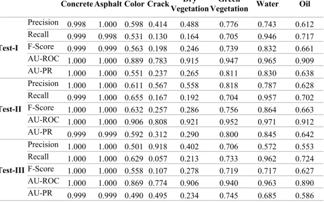
To proceed with the modeling and performance evaluation, a data partition strategy is needed to split the data; hence one part is for the training and the other for model validation. In the literature, the widely used scheme is to use 75% of the total data for training and the rest 25% for testing. Indeed, if there are sufficient amount of data, the data splitting ratio is flexible and up to the analyst. In this paper, it is meaningful to examine if the data size is sufficient, which can be reflected if the prediction performance increases with the size of training data. Three data splitting schemes are considered for any of the obtained feature dataset as expressed above. In the first scheme namely Test-1, and by carrying out a random shuffling, 25% (8147) of the data set is considered for training and the rest 75% (26601) for testing purposes. In Test-2, the total dataset is divided equally (i.e., 17374 for training and testing, separately). In Test-3, 75% (26601)

(51)

41

of the dataset is considered for training and the rest 25 % (8147) for testing. With these three schemes, a total of 12 different models are evaluated in this thesis work.

The accuracy of the classifier needs to be defined for estimating and comparing the quality of the classification result. In this effort, due to the presence of a higher number of classes, it is important to properly analyze each parameter as a higher number of classes in general decrease the classification accuracy. To quantify the performance of the classifiers and more importantly their predictive capacity and robustness, two commonly used performance analytics, receiver operating characteristics (ROC) curve, and

precision-recall (PR) curve, are adopted, which are constructed by setting a variable decision threshold in the classifier. The area under ROC (AU-ROC) and precision-recall (AU-PR) curve are