Production Scheduling and Rescheduling with Genetic Algorithms

Genetic Algorithms

Christian Bierwirth University of Bremen Department of Economics Box 330440 D-28334 Bremen, Germany [email protected] Dirk C. Mattfeld University of Bremen Department of Economics Box 330440 D-28334 Bremen, Germany [email protected] Abstract

A general model for job shop scheduling is described which applies to static, dynamic and non-deterministic production environments. Next, a Genetic Algorithm is presented which solves the job shop scheduling problem. This algorithm is tested in a dynamic environ-ment under different workload situations. Thereby, a highly efficient decoding procedure is proposed which strongly improves the quality of schedules. Finally, this technique is tested for scheduling and rescheduling in a non-deterministic environment. It is shown by experi-ment that conventional methods of production control are clearly outperformed at reasonable runtime costs.

Keywords

Genetic algorithm, permutation representation, tunable decoding, job shop scheduling prob-lem, dynamic scheduling.

1 Introduction

With the spread of automated manufacturing systems the optimization problem of assigning operations to a set of machines receives increasing attention (Parunak, 1992). From the viewpoint of combinatorial optimization the issue of finding an optimal production schedule is known to be

NP

-hard (Błazewicz et al., 1996). Therefore particular attention is paid to local search-based heuristics (Anderson et al., 1997) including Genetic Algorithms (GA). A good deal of previous research on GAs in scheduling concentrates on the static job shop prob-lem (Mattfeld, 1996). However, production is an activity of sustained pursuit and therefore production scheduling is actually a dynamic task.

In a manufacturing system all jobs have release times which define their date of arrival at the shop floor. Job releases are typically unforeseen events and, consequently, neither the release times of jobs nor their specific processing requirements are known in advance. Therefore, scheduling is a non-deterministic problem dealing with an open time horizon. The control of the jobs in a manufacturing system is referred to as rescheduling because unforeseen events frequently require schedule revisions.

In practice predominantly priority-rule based control is used (Baker, 1974). The temporal decomposition of the non-deterministic problem into a series of dynamic, but deterministic

problems also opens this domain for optimization methods (Raman and Talbot, 1993). Since already small improvements of the schedule quality obtained by optimization often lead to considerable cost reductions, advanced optimization techniques are highly appreciated. The transfer of GA experiences to production control was first approached in Bierwirt et al. (1995) and has been taken up recently in Lin et al. (1997) by addressing the GA effectiveness. We think that the GA efficiency is of predominant importance. So far, however, the GA runtimes have hindered a thorough computational study as usually done for priority-rule based scheduling.

This paper proposes an optimization method for the problem sketched above. In Sec-tion 2 we first review the static job shop problem. Next we extend the static scheduling problem to a dynamic one. In Section 3 we present a GA capable of solving the dynamic job shop problem. In Section 4 a highly efficient decoding procedure is presented and evaluated by experiment. In Section 5 the GA is applied to rescheduling and tested in two variants of which one again improves the GA efficiency. The results are compared with the outcome of priority-rule based scheduling before we conclude in Section 6.

2 Job Shop Scheduling

2.1 The Static Model

The static model for job shop scheduling describes a simplified multistage production process. We consider a manufacturing system consisting of

m

machines

M

₁

;:::M

m

for which several assumptions are made. Machines cannot substitute each other and there is no preemption of a processing unit. In this ideal system no machine breakdowns occur and the passing times of jobs between machines are neglected. Furthermore, job-specific setup times of machines are not considered.

A production program consists of

n

jobs

J

₁

;:::J

n

and each job consists of at most

m

operations. All operations have to be processed by dedicated machines but no job has to be processed twice by the same machine. The actual number of operations of job

J

i

(1

i

n

)

is

denoted by

m

i

. Since the jobs do not necessarily have to pass every machine,

m

i

m

holds.

Each job

J

i

defines a production recipe

i

given as an order of the machines it has to pass. The vector

i

points to the machines, hence for

i

(

k

) =

j

(1

k

m

i

)

machine

M

j

is the

k

-th machine that processes

J

i

. The

k

-th operation of job

J

i

processed on machine

M

i(

k

)is

denoted as

o

ik

. The required processing time of

o

ik

is known in advance and denoted by

p

ik

. A schedule of a production program can be seen as a table of starting times

t

ik

for the operations

o

ik

with respect to the technological machine orders of jobs. The completion time of an operation is given by its starting time plus its processing time

(

t

ik

+

p

ik

)

. The earliest possible starting time of an operation is determined by the maximum of the completion times of the predecessor operations of the same job and of the same machine. Hence the starting time for operation

o

ik

is calculated by

t

ik

= max

t

i;k

,1

+

p

i;k

,1

; t

hl

+

p

hl

:

(1)

Here

o

hl

refers to the operation of job

J

h

which precedes

o

ik

on its machine, i.e.

i

(

k

) =

h

(

l

)

. For

k

= 1

we deal with the beginning operation of a job and therefore in this case the first argument in the max-function is set to zero. If

o

ik

is the first operation processed on a machine it has no machine predecessor and now the second argument in the max-function is set to zero.

The completion time

C

i

of a job

J

i

is given by the completion time of its final operation

o

i;m

i, i.e.

C

i

=

t

i;m

i

+

p

i;m

i. As a measure of the performance of a schedule often the

minimization of

C

_max

= max

f

C

1

;:::C

n

gis pursued. This objective function is optimized by

reducing the time span needed in order to make the entire production program.

2.2 The Dynamic Model

We now consider an extension of the static model in which the

n

jobs are released at different points in time. The release time

r

i

of job

J

i

determines the point in time at which

J

i

arrives in the shop floor. The starting time of the beginning operation of a job is now given by the maximum of the release time and the completion time of its machine predecessor operation

o

hl

t

i

1

= max

r

i

; t

hl

+

p

hl

:

(2)

The non-beginning operations of

J

i

are still scheduled according to equation (1). When-ever release times are taken into account for building a schedule, the job shop model is referred to as a dynamic one. Here, we still assume that all release times are known in advance. There-fore, we classify this type of job shop to be dynamic, but deterministic.

In the dynamic model

C

_max predominantly depends on the release time of the latest released job. Therefore it cannot serve as a proper measure of performance anymore. Instead, the mean flow-time of jobs is used. It is calculated by

F

=

1

n

P

n

i

=1

C

i

,

r

i

. Minimizing

F

seeks to complete jobs as soon as possible. In practice short job flows are preferred because they reduce the work in progress inventory costs and increase the flexibility within the shop floor.

2.3 The Non-Deterministic Model

Since production is an activity of sustained pursuit, scheduling of the production process is a non-deterministic problem. The production process is typically supposed to last beyond the completion of any of the known jobs. Therefore scheduling deals with an open time horizon. We follow Raman et al. (1993) to handle situations where jobs arrive non-deterministically in the manufacturing system. In their approach the non-deterministic scheduling problem is decomposed into a sequence of dynamic but deterministic scheduling problems.

Let

P

0be a dynamic job shop problem as introduced in Section 2.2.

P

0arises from the release of a production program at time

t

0

= 0

. At

t

0the program consists of

n

jobs. Up to the next release of new jobs at time

t

₁

> t

₀problem

P

₀can be solved. This leads to a table of potential starting times for all operations involved in

P

₀.

To construct the new problem

P

₁we make a snapshot at the release time of new jobs

t

₁. The operations

o

ik

with potential starting times

t

ik

< t

₁have already been implemented in the manufacturing system and are, therefore, now removed from the problem. We modify the jobs

J

i

of

P

₀which cover operations starting in the period from

t

₀to

t

₁. Then we remove the corresponding operations from the technological machine order and finally decrease

m

₁ to the number of remaining operations of job

J

i

. If

m

i

= 0

we remove job

J

i

completely. If a job has been modified but not removed from the production program we calculate a new release time for the modified job

J

i

by

r

i

= max

₁

k

m

i n

t

ik

+

p

ik

j

t

ik

< t

1 o

:

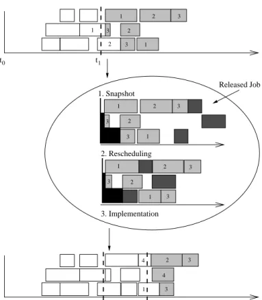
(3)

Released Job 1. Snapshot 2. Rescheduling 0 t 0 t t₁ t₁ t₂ 3. Implementation 3 1 2 3 1 2 3 2 2 1 3 2 1 1 2 2 3 3 1 2 3 4 3 4 1 1 3 3 M M M₁ 2 3 M M M₁ 2 3 3

Figure 1: Production scheduling on a rolling time basis.

Figure 1 shows a snapshot of a manufacturing system at time

t

₁. The operations which have not been started before

t

₁appear in light grey shade. Sometimes the processing of an operation

o

ik

, starting shortly before a new job is released, overshoots

t

₁(

t

ik

< t

₁

< t

ik

+

p

ik

). In this situation

M

i(

k

)is not available at time

t

1. In the charts this is depicted by black shadings

on

M

₂and

M

₃. To model the situation of non-availability of machines we introduce initial setup times

s

j

for the machines

M

j

(1

j

m

)

. The setup times

s

j

denote the earliest point

in time machine

M

j

is available again. It is calculated by

s

j

= max

max

1

i

n

t

ik

+

p

ik

j

t

ik

< t

1

; t

1

:

(4)

Finally, we add the jobs which are released in the shop floor at time

t

₁to the remaining production program. In Figure 1 one job depicted in dark grey shade is appended. The updated production program results in a new dynamic scheduling problem

P

1. Next, the production program can be rescheduled. Thereby the machine setup times

s

j

are taken into account when using machine

M

j

for the first time. If any operation

o

ik

with

i

(

k

) =

j

is the first operation processed by

M

j

we set

t

ik

= max

t

i;k

,1

+

p

i;k

,1

; s

j

:

(5)

being those operations that both a) begin a job and b) are processed as the first operation on their machine. For these operations starting times are calculated by

t

ik

= max(

r

i

;s

i(

k

)

)

.

Until further jobs are released at

t

₂, all operations scheduled before

t

₂can be implemented in the manufacturing system. Repeating this procedure after each new job release, the production program is rescheduled periodically on a rolling time basis.

3 Genetic Algorithm Design

GA approaches to the dynamic job shop problem are scarce. In addition to our previous work (Bierwirth et al., 1995) two further approaches are known from literature (Fang et al., 1996; Lin et al., 1997). In the following a new GA capable of solving the dynamic job shop problem is described. It combines well known components adopted from previous research in the fields of Operations Research and Evolutionary Computation into a very efficient algorithm. First, the solution encoding and the genetic operators, all of them already proven suc-cessful, are sketched. Next a decoding procedure previously proposed by Storer et al. (1992) is introduced in detail. Finally the parameterization of the algorithm is described.

3.1 The Encoding and Operators

Encoding. The encoding of solutions to a problem should ensure that all possible solutions can be generated provided that chromosomes are generated at random. For combinatorial ordering problems, usually permutation encodings are used, because the order of items can be most naturally modeled in this way. Here, the order within the permutation is interpreted as a sequence while scanning it from left to right in the decoding step.

For our purpose, we use a permutation of all operations involved in an instance of a scheduling problem. The order of operations in the permutation serves as a sequence for the decoding procedure which consecutively assembles a schedule from this information. Note that not all permutations represent feasible schedules directly. An operation is schedulable only if its job predecessor has been scheduled already, i.e. a job predecessor of an operation must occur on the left hand side of its position in the permutation. In our approach we neglect this restriction and feasibility is ensured by the decoding procedure.

Crossover. Recombination plays a crucial role for the GA performance. According to the widely accepted design goal for crossover operators, information already existing in the parent solutions should be recombined without introducing new information. For the job shop scheduling problem the precedence relations of an operation to other operations projected for the same machine is of particular importance. This information should be passed on in order to produce competitive offspring.

In the following we describe the Precedence Preservative Crossover (PPX) which was independently developed for vehicle routing problems by Blanton and Wainwright (1993) and for scheduling problems by Bierwirth et al. (1996). The operator passes on precedence relations of operations given in two parental permutations to one offspring at the same rate, while no new precedence relations are introduced. PPX is illustrated in Figure 2 for a problem consisting of six operations A-F.

The operator works as follows: A vector of lengthP

n

i

=1

m

i

, representing the number of operations involved in the problem, is randomly filled with elements of the setf

1

;

2

g. This

vector defines the order in which the operations are successively drawn from parent 1 and parent 2. We can also consider the parent and offspring permutations as lists, for which the

parent permutation 1 A B C D E F

parent permutation 2 C A B F D E

select parent no. (1/2) 1 2 1 1 2 2

offspring permutation A C B D F E

Figure 2: Precedence Preservative Crossover.

operations ’append’ and ’delete’ are defined. First we start by initializing an empty offspring. The leftmost operation in one of the two parents is selected in accordance with the order of parents given in the vector. After an operation is selected it is deleted in both parents. Finally the selected operation is appended to the offspring. This step is repeated until both parents are empty and the offspring contains all operations involved. Note that PPX does not work in a uniform-crossover manner due to the ’deletion-append’ scheme used.

Mutation. This operator should alter a permutation only slightly. The rationale behind this idea is that a small modification in the permutation will result in a small deviation of its fitness value only. In this way the information newly introduced by a mutation has a reasonable chance to be selected and accordingly passed on into future generations.

In our GA we alter a permutation by first picking (and deleting) an operation before reinserting this operation at a randomly chosen position of the permutation. In doing so, at the extreme, all precedence relations of one operation to all other operations are modified. Typically such a mutation has a much smaller effect and often it does not even change the fitness value.

3.2 The Permutation Decoding

Permutations can be decoded into semi-active, active or non-delay schedules. The three properties of schedules are achieved by incorporating domain knowledge such that the size of the search space is continuously reduced. A comparative description of these procedures is given below.

Semi-active. Schedules are built by successively scheduling the operations by assigning the earliest possible starting time according to Equation 1. The permutation to be decoded serves as a look-up array for the procedure described below. In this way the procedure schedules the operations in the order given in the permutation.

However, an operation

o

ik

found in the permutation is only schedulable if its job prede-cessor

o

i;k

,1has been scheduled already. Therefore in a feasible permutation

o

i;k

,1 occurs

to the left of

o

ik

. In the case of infeasible permutations the decoding procedure ensures feasibility of the resulting schedule by delaying an operation until its job predecessor has been scheduled.

1. Build the set of all beginning operations,

A

:=

f

o

i

1j

1

i

n

g.

2. Select operation

o

ik

from

A

which occurs leftmost in the permutation and delete it from

A

,

A

:=

A

nf

o

ik

g.

3. Append operation

o

4. If a job successor operation

o

i;k

+1 of the selected operation

o

ik

exists, insert it into

A

,

A

:=

A

[f

o

i;k

+1g.

5. If

A

6

=

;goto Step 2, else terminate.

Depending on whether the problem under consideration is static, dynamic or non-deterministic, the earliest possible starting times of operations are calculated by Equations (1), (2) and (5) respectively.

Active. Active schedules are produced by a modification of Step 2 in the above procedure which leads to the well known algorithm of Giffler & Thompson (1960).

2.A1 Determine an operation

o

0

from

A

with the earliest possible completion time,

t

0

+

p

0

t

ik

+

p

ik

for all

o

ik

2

A

.

2.A2 Determine the machine

M

0

of

o

0

and build the set

B

from all operations in

A

which are processed on

M

0

,

B

:=

f

o

ik

2

A

j

i

(

k

)

=

M

0

g.

2.A3 Delete operations in

B

which do not start before the completion of operation

o

0

,

B

:=

f

o

ik

2

B

j

t

ik

< t

0

+

p

0

g

:

2.A4 Select operation

o

ik

from

B

which occurs leftmost in the permutation and delete it from

A

,

A

:=

A

nf

o

ik

g.

This algorithm produces schedules in which no operation could be started earlier without delaying some other operation or breaking an order constraint. Notice that active schedules are also semi-active schedules.

Non-delay. Schedules are produced similarly by using a more rigid criterion for picking an operation from the so called critical set

B

. Modify Step 2 as follows:

2.N1 Determine an operation

o

0

from

A

with the earliest possible starting time,

t

0

=

t

ik

for all

o

ik

2

A

.

2.N2 Determine the machine

M

0

of

o

0

and build the set

B

from all operations in

A

which are processed on

M

0

,

B

:=

f

o

ik

2

A

j

i

(

k

)

=

M

0

g.

2.N3 Delete operations in

B

which start later than operation

o

0

,

B

:=

f

o

ik

2

B

j

t

ik

=

t

0

g

:

2.N4 Select operation

o

ik

from

B

which occurs leftmost in the permutation and delete it from

A

,

A

:=

A

nf

o

ik

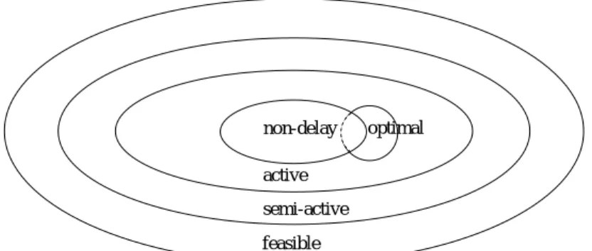
g.

Non-delay scheduling means that no machine is kept idle when it could start processing some operation. Non-delay schedules are necessarily active and hence also necessarily semi-active. This property is illustrated in Figure 3. Concerning the minimization of

C

_maxand

F

it is well known that at least one of the optimal schedules is an active one. Unfortunately there is not necessarily an optimal schedule in the set of non-delay schedules. However, there is strong empirical evidence that non-delay schedules show a better mean solution quality than active ones. Nevertheless, scheduling algorithms typically search the space of active schedules in order to guarantee that the optimum is taken into consideration.

Numerous GA approaches to job shop scheduling have used an active scheduler, e.g. (Yamada and Nakano, 1992; Dorndorf and Pesch, 1995). Contrarily, a non-delay scheduler

optimal non-delay

active semi-active feasible

Figure 3: Relationships of schedule properties.

has been used in the decoding procedure of a GA by Della Croce et al. (1995). They report that a non-delay scheduler can improve the solution quality for some problem instances whereas for others the active scheduler succeeds. As a remedy Della Croce et al. augment the non-delay scheduler with a so called “look ahead” strategy. This strategy is driven by the operation sequence in the permutation and can accept that a machine runs idle although it could start processing an operation. The authors report, that “looking ahead” widens the search space in most cases, but does not codify all the active schedules. In this paper we implement a similar, but tunable hybrid scheduler previously proposed by Storer et al. (1992).

Hybrid. Hybrid schedules can be produced in a flexible way by introducing a tunable parameter

2

[0

;

1]

. The setting of

can be thought of as defining a bound on the length of

time a machine is allowed to remain idle. At the extremes

= 0

produces non-delay schedules while

= 1

produces active schedules. For the details of an efficient implementation of this algorithm in order

O

(

n

2

)

the reader is referred to Storer et al. (1992). Below we give a version of the hybrid scheduler in terms of the framework already used above:

2.H1 Determine an operation

o

0

from

A

with the earliest possible completion time,

t

0

+

p

0

t

ik

+

p

ik

for all

o

ik

2

A

.

2.H2 Determine the machine

M

0

of

o

0

and build the set

B

from all operations in

A

which are processed on

M

0

,

B

:=

f

o

ik

2

A

j

i

(

k

)

=

M

0

g.

2.H3 Determine an operation

o

00

from

B

with the earliest possible starting time,

t

00

=

t

ik

for all

o

ik

2

B

.

2.H4 Delete operations in

B

in accordance to parameter

such that

B

:=

f

o

ik

2

B

j

t

ik

<

t

00

+

((

t

0

+

p

0

)

,

t

00

)

g.

2.H5 Select the operation

o

ik

from

B

which occurs leftmost in the permutation and delete it from

A

,

A

:=

A

nf

o

ik

g.

3.3 The Parameterization of the Algorithm

Thus far we have described major components for a GA capable of solving dynamic job shop scheduling problems. These components are now embedded into the framework of a simple GA. The mean flow time of jobs directly serves as the fitness of schedules. Since we minimize fitness, selection is based on inverse proportional fitness. The PPX operator is applied with

probability

0

:

8

, whereas the mutation operator is applied with the relatively high probability of

0

:

2

. We use a fixed population size of 100 individuals.

The hybrid scheduler is engaged as the decoding procedure. After a permutation has been decoded, the permutation is rewritten with the sequence of operations as they actually have been scheduled. This feature was first used by Nakano and Yamada (1991) under the name “forcing”. In order to take advantage from a fast convergence, a flexible termination criterion is used. The algorithm terminates after a number of generations

T

which are carried out without gaining any further improvement. We confine

T

to the number of jobs contained in a problem instance. In this way larger instances are given a reasonably longer time to converge.

4 GA based Scheduling

The lack of scalability of GAs for scheduling is known as a central weakness in comparison to other proposed methods. This finding is verified in Mattfeld (1996) by a comprehensive study on large-scale benchmarks for static job shop scheduling proposed by Taillard (1993). For 80 problem instances consisting of 225 up to 2000 operations a GA produced a continuously increasing relative error against the best known solutions ranging from 2.03% to 7.59% respectively. Apparently, the capability of GAs for converging to near-optimality vanishes with increasing problem size. We address this issue by an investigation on the hybrid scheduler. First we reveal the GA weakness before we propose a suitable setting for the tunable parameter of the hybrid scheduler.

4.1 Improving Efficiency by Hybrid Scheduling

The appropriate setting of the parameter

, which controls the hybrid scheduler, remains as an open issue. Storer et. al propose values of 0.0 and 0.1 in the context of a different search method. In order to derive a suitable parameterization in the context of GAs, we proceed a computational study in this section. But let us first discuss the influence of the hybrid scheduler on the GA performance.

Let us suppose that the GA has the potential to converge to optimality for a problem of a certain size. If the GA uses the active scheduler (

= 1

), the GA is likely to find the optimal solution. If, however, the GA uses the non-delay scheduler (

= 0

) the solution found is probably of inferior quality because non-delay scheduling may have excluded the optimum from the search space. On the other hand, the algorithm will converge faster if non-delay scheduling is used. Thus we face a tradeoff between the runtime and the solution quality achieved.

Let us change the above assumption in supposing that the GA is likely to converge prematurely for a problem of a certain size, i.e. the optimum will not be found. In this case, reducing the size of the search space by using the non-delay scheduler may lead to better results compared to those achieved by the active scheduler, although the optimal solution may be excluded from search. The property of a faster convergence for the non-delay scheduler remains undeterred for this scenario.

In consequence, for the hybrid-scheduler the choice of

can have a strong influence on the quality achieved as well as on the runtime required by the GA. For an appropriate setting of the parameter within the range

0

1

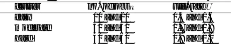
we proceed with a computational study.

Table 1: Three cluster of test problem instances.

cluster no. of jobs

n

util. rate

U

easy 10 and 20 0.5 and 0.6

moderate 30 and 40 0.7 and 0.8

hard 50 and 60 0.9 and 1.0

4.2 Experimental Setup

In order to assess the influence of the decoding procedure on the GA performance we refer to an experimental environment which is often used in literature for simulating manufacturing systems (see e.g. Holthaus & Rajendran (1997)).

Care is taken to model the arrival process of jobs in the manufacturing system. The inter-arrival times of jobs affect the workload of the manufacturing system. The workload is defined as the number of operations in the system which await processing. While modeling a dynamic manufacturing system, the mean inter-arrival time

can be prescribed by dividing the mean processing time of jobs

P

by the number of machines

m

and a desired utilization rate

U

, i.e.

=

P=

(

mU

)

. We simulate a simplified manufacturing system by using the following attributes:

1. The manufacturing system consists of 6 machines.

2. Each job passes 4 to 6 machines resulting in 5 operations on average.

3. The machine order of operations within a job is generated from a uniform probability distribution.

4. The processing times of operations are uniformly distributed in the range of

[1

;

19]

which leads to a mean processing time of

P

= 5

10

.

5. We generate exponentially distributed inter-arrival times based on

by using various utilization rates

U

.

We vary the number of jobs

n

between 10 and 60 in steps of 10. The utilization rate

U

is varied between 0.5 and 1.0 in steps of 0.1. For each of the four combinations of

n

and

U

shown in Table 1 we generate 25 instances at random. These instances are divided into three clusters, each containing 100 problem instances. “Easy” instances consists of a few jobs only which are released with loosely set inter-arrival times. “Hard” instances consists of many jobs which arrive tight after another. An increasing

U

leads to a decreasing

which in turn results in a larger number of operations to be scheduled simultaneously. In short, a large

U

generates difficult problems and vice versa. In this way more or less challenging problem instances are generated.

The GA is run 10 times for all instances and for all

2f

0

;

0

:

1

;

1

g. These

10

300

11

results are separated according to their dedicated cluster. Within each cluster the mean for each

is produced over the corresponding

10

100

results. Finally, the 11 values achieved

for each cluster are normalized to the range

[0

;

1]

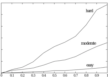
in order to enable comparisons concerning

-0.1 0 0.1 0.2 0.3 0.4 0.5 0.6 0.7 0.8 0.9 1 0 0.1 0.2 0.3 0.4 0.5 0.6 0.7 0.8 0.9 1 moderate hard normalized flow-time easy δ

Figure 4: Influence of hybrid-decoding on GA performance.

4.3 Results and Discussion

The results shown in Figure 4 verify the conjecture made in Section 4.1 suggesting that the proper functioning of GAs for scheduling is limited to a certain size of the search space. Starting from non-delay scheduling with

= 0

, the increase of

leads to improved solutions in all three clusters. Here, previously excluded solutions are now included into the scope of the search while the GA still works sufficiently well. Beyond a borderline a further increase of

leads to a deterioration of the solution quality although potentially better solutions are included into the search space. Obviously, the increasing size of the search space cannot be handled properly by the GA anymore.

We find different values of

to be most suitable for the three clusters, namely 0.4 for “hard”, 0.5 for “moderate”, and 0.7 for “easy” problem instances. To explain this difference, recall that the size of the search space is determined by the

chosen and, of course, by the size of the problem instance. Given a problem of fixed size, an increasing

enlarges the search space beyond a borderline, where the potentials of the GA are exceeded. Obviously, this happens earlier for harder problems because they are of larger size.

One can easily identify that the worst level of solution quality for “easy” problems is produced with non-delay scheduling, while active scheduling still results in a reasonable solution quality. For the “hard” problem instances things are just the other way round. In the case of extremely large problems

close to 0 may work best. In the following we use

= 0

:

5

which produces above average results for all three cluster investigated.

As it has turned out from our above discussion, the active scheduler will need more generations compared to its non-delay counterpart in order to drive the GA to convergence. Accordingly, a GA using an active scheduler is more time consuming. We now reveal the impact of the hybrid scheduling on the GA runtime. Figure 5 depicts the development of the number of generations needed until termination.

For this purpose we subtract the number of generations spent with non-delay scheduling from the number of generations spent with values of

>

0

. This presentation focuses on the possible acceleration of the GA achieved by hybrid scheduling. As one would expect,

0 50 100 150 200 250 300 0 0.1 0.2 0.3 0.4 0.5 0.6 0.7 0.8 0.9 1 easy moderate hard generations δ

Figure 5: Influence of hybrid-decoding on GA generations.

a continuous increase of the number of generations can be seen for increasing

values. At

= 0

:

5

less than the half of generations are needed compared to active scheduling.

Summarizing, a hybrid scheduler parameterized with

= 0

:

5

yields an improved solution quality by saving a significant amount of runtime at the same time. If runtime is the limiting resource, one might think of using a smaller

value in order to speed up the search. Particularly for large problems the expected loss of solution quality for

<

0

:

5

seems to be bounded. 5 GA based Rescheduling

The GA outlined in the previous section is now used to solve a series of dynamic problems resulting from a temporal decomposition in a non-deterministic environment (Raman and Talbot, 1993). Now the GA actually reschedules the production program as it is sketched in Figure 1.

5.1 Improving Efficiency by Biasing the Search

The simplest approach to using the GA for rescheduling is to make a snapshot of the manufac-turing system and to formulate a corresponding dynamic, but deterministic problem. Starting with a randomly generated population, the GA solves this problem and returns the best solu-tion found. This solusolu-tion is implemented in the manufacturing system as far as possible with respect to a forthcoming snapshot. In this manner the GA is restarted after each snapshot taken at the arrival of a new job.

A more sophisticated approach proposed is to reuse some of the work already done (Fang et al., 1993; Bierwirth et al., 1995). Whenever a new job arrives at time

t

, a new problem is created like described above. Different from the previous approach, the population of the newly started GA is now obtained from the final population of the previous GA by adjusting it to the requirements of the new problem, see Section 2.3. In other words, the search process is given a bias by seeding the initial population instead of initializing it at random. The adjustment of the population requires two steps.

1. The operations which have been started before

t

, including those which are still processed, are deleted in all permutations of the population.

2. The operations of new jobs are inserted at random positions in all permutations of the population respecting the job’s operation order.

Furthermore, job release times and machine setup times are updated using Equations (3) and (4). The operations already started before time

t

are not considered any longer. Whenever the final operation of a job is eliminated in this way, the job itself vanishes completely. After all these modifications, the GA continues the optimization process.

Now the initial population contains fragments of favorable solutions found in the previous GA run. We conjecture that these fragments resemble each other strongly, because, due to the termination criterion described in Section 3.3, the population of the previous problem is likely to have already converged regardless of the size of this problem. Therefore biasing the population will lead to a faster convergence which in turn will result in a considerable saving of runtime (Grefenstette, 1987).

Regarding the quality achieved we see two possible impacts: The information transferred may concentrate the search on parts of the search space which are still promising in the current situation. On the other hand, the similarity of individuals in the biased population may hinder a thorough search. This issue is subject to a computational investigation.

5.2 Experimental Setup

We run the decomposition by using both variants of the GA and compare the outcome in terms of solution quality and runtime. Jobs are generated in the same way as done in the experimental setup described in Section 4.2. This time we use slightly different utilization rates which correspond to reasonable workloads of a manufacturing system. Utilization rates of

U

2f

0

:

65

;

0

:

70

grepresent a relaxed situation of the manufacturing system. A moderate

load is produced by

U

2f

0

:

75

;

0

:

80

gwhereas utilization rates of

U

2f

0

:

85

;

0

:

90

gproduce an

excessive workload.

Modeling the inter-arrival times by a Possion process as described in Section 4.2 can lead to extreme deviations of the workload in different phases of the simulation run. Therefore a large variance of both, the quality achieved as well as the runtime required can be observed. In order to alleviate this effect, a large number of job releases has to be simulated. Moreover, a large number of different simulations is needed in order to produce a sound overall mean. Consequently, for each

U

investigated we conduct 50 simulation scenarios consisting of

1000

jobs each.

In a preliminary investigation we run the non-delay scheduler described in Section 3.2. Thereby the selection of an operation from the critical set (Step 2.N4) gives priority to the operation with the shortest imminent processing time (SPT). Jobs waiting in a queue may cause their dedicated successor machines to run idle. The SPT rule alleviates this risk by reducing the length of the queues in the fastest possible way. This in turn reduces the complexity of the manufacturing system. For this reason SPT dominates all other existing priority rules if the minimization of

F

is pursued.

SPT runs are carried out for all utilization rates prescribed. Thereby the workload observed in the system is recorded. Keep in mind that the workload of the decomposed deterministic problem is simply the number of the operations involved.

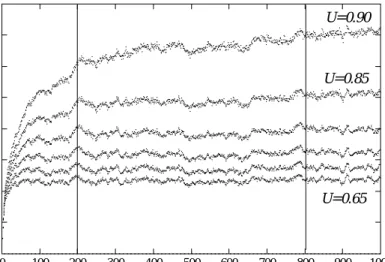
0 10 20 30 40 50 60 70 80 0 100 200 300 400 500 600 700 800 900 1000

workload in the system

number of released jobs

U=0.90

U=0.85

U=0.65

Figure 6: System workload under SPT-based control.

six utilization rates used. Consider the development of the workload in the early phase of the simulation. The workload continuously increases until a stationarity is reached (apart from

U

= 0

:

90

) after approximately 200 job releases. Notice, that the difference between adjacent levels of stable workload increases with

U

. This observation indicates that a small additional increase of the workload may not be handled properly in a tense production situation anymore. Therefore, for

U

= 0

:

90

, a stabilization of the workload cannot be observed within the 1000 jobs released.

The figure depicts that jobs scheduled in the early phase of the simulation distort the

F

measure considerably. The same is true for the final phase of the simulation run. Consider the last problem constituted at job release 1000. Although it still consists of many operations, it must be solved entirely now. By taking these effects into account, we must doubt the results reported by Lin et al. (1997) for a similar study. The scenarios investigated by Lin et al. consist of 100 job releases — the leftmost 10% of job releases shown in Figure 6. In our computational study we discard job 1 to 200 as well as job 801 to 1000 from being evaluated in order to circumvent distortion effects.

5.3 Results and Discussion

After we have carefully designed the experiment, we perform simulation runs for both GA variants described in Section 5.1. The randomly initialized GA is called “rand” and its seeded counterpart is called “bias” in Table 2. The mean flow-times of jobs achieved for the SPT rule and both GA variants are reported. For the GAs also the average number of generations and the average runtime of a simulation scenario are listed. The programs are run on a Pentium/200 Mhz computer.

From Table 2 we see that the flow-times of jobs obtained by SPT increase strongly with the utilization rate. Under high utilization rates the large workload results in long flow-times of jobs. The prescribed average processing time

P

= 50

of jobs can serve as a simple lower bound for

F

. By subtracting this value from

F

we obtain the average waiting time of a job in the system which increases from

42

for

U

= 0

:

65

up to

150

units for

U

= 0

:

90

.

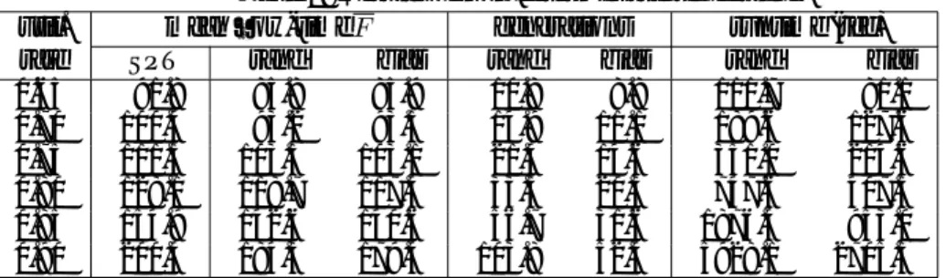
Table 2: Results of non-deterministic scheduling.

util. mean flow-time

F

generations runtime (sec)

rate SPT rand bias rand bias rand bias

0.65 91.8 85.8 85.9 10.8 8.8 111.7 81.1 0.70 100.4 93.2 93.5 14.9 11.1 189.6 127.6 0.75 111.5 103.5 103.1 21.4 14.6 351.0 214.6 0.80 128.1 118.7 117.4 33.5 20.3 747.6 407.5 0.85 154.9 142.6 140.6 56.7 31.6 1876.4 953.0 0.90 200.4 184.3 179.4 103.8 52.4 5928.1 2705.5

The SPT rule is outperformed by both GA variants for all utilization rates tested. Thereby a reduction of 15% of the waiting time of the jobs is gained for all values of

U

. The solution quality produced by the GA variants differ only slightly from each other. As it can be taken from the lower curve in Figure 6, the dynamic problems solved under

U

= 0

:

65

consists of about 25 operations. For such small problems both versions of the GA come up with almost identical results. With an increasing

U

the problem size increases and now the biased GA dominates its rival by a few percent.

Table 2 also reports the average number of generations performed in the GA runs until termination occurred. Recall the flexible termination criterion used. For

U

= 0

:

65

the biased GA uses slightly less generations than its randomly initialized counterpart. In contrast, for a heavily loaded system, the unbiased GA demands up to two times the generations needed when used on a biased basis. The larger the workload increases, the more advantageous the biasing of the initial GA population gets in terms of the generations spent.

The advantage becomes even more clear by considering the runtime required for one simulation scenario. Note that the time needed by the hybrid scheduler increases at

O

(

n

2

)

with the problem size. For

U

= 0

:

90

the GA solves problems of an average size of 73.5 operations. The “rand” GA is clearly outperformed by its “bias” rival. Even under heavy load only 2705.5 seconds are spent on average by the biased GA in order to solve 1000 subsequent problems. Thus, the rescheduling of the system is performed competitively fast in 2.7 seconds. In order to derive the runtime of the SPT-scheduler recall that a priority rule just determines the order of operations in the scheduler. The same scheduler evaluates the fitness within the GA, this time driven by the order of operations in the permutation. Since the population consists of 100 permutations and the biased GA performs 52.4 generations on average for

U

= 0

:

90

, we can easily examine that a priority rule based scheduler performs at least 5240 runs in a time span of 2.7 seconds. Thus we must admit that priority based scheduling requires a fraction of a second only. However, the results presented justify the additional time spent for the biased GA.

6 Summary and Conclusion

Throughout the last decade numerous GA approaches to production scheduling have been reported. These approaches differ strongly from each other with respect to the encoding and operators used, the constraints handled and the goals pursued. Despite these differences, all approaches have in common that domain knowledge is required in order to produce competitive schedules. Although highly desirable, the GA is not capable to conduct the search properly.

have been proposed. Probably the most successful approach is to introduce hill-climbing resulting in a genetic local search approach. Unfortunately, for most scheduling problems hill-climbing lacks an efficient estimate of promising neighborhood moves. For these cases the remedy of reducing the search space by means of an active scheduler has been proven successful.

Despite searching in the set of active schedules only, the capabilities of the GA to conduct a proper search still vanish with an increasing problem size. This weakness of GA based scheduling can be alleviated by a further reduction of the search space. For this end we have proposed a tunable decoding procedure which proportions the size of a search space within useful bounds. Although this procedure may exclude optimal and even near optimal solutions from being searched, the positive effects of the search space reduction do prevail. Moreover, the GA runtime is reduced by approximately 50%.

A temporal decomposition of a non-deterministic production environment opens this domain for GA based scheduling. One way to a further reduction of the computational effort is to fall back on information available at no cost. Based on this principle a rescheduling of the current problem is done whenever a new job is released. Thereby the initial population of the GA is built by modifying the final population of the preceding GA run. Again, this technique cuts down the GA runtime by about one half.

In this paper we have dealt with the minimization of the mean flow-time of jobs, because for this objective the excellent performance of the SPT rule is well known. Against this simple but powerful rival, the GA approach produces far better results at a reasonable runtime. References

Anderson, E. J., Glass, C. A., and Potts, C. N. (1997). Machine scheduling. In Aarts, E. H. L. and Lenstra, J. K., editors,Local Search Algorithms in Combinatorial Optimization, pages 361–414, John Wiley, New York, New York.

Baker, K. R. (1974).Introduction to Sequencing and Scheduling, John Wiley, New York, New York. Bierwirth, C., Kopfer, H., Mattfeld, D. C., and Rixen, I. (1995). Genetic algorithm based scheduling

in a dynamic manufacturing environment. In Palaniswam, M., editor, Proceedings of the Second Conference on Evolutionary Computation, pages 439–443, IEEE Press, New York, New York. Bierwirth, C., Mattfeld, D., and Kopfer, H. (1996). On permutation representations for scheduling

problems. In Voigt, H.-M., et al., editors,Proceedings of Parallel Problem Solving from Nature IV, pages 310–318, Springer Verlag, Berlin, Germany.

Blanton, J. L. and Wainwright, R. L. (1993). Multiple vehicle routing with time and capacity constraints using genetic algorithms. In Forrest, S., editor,Proceedings of the Fifth International Conference on Genetic Algorithms, pages 452–459, Morgan Kaufmann, San Mateo, California.

Błazewicz, J., Domschke, W., and Pesch, E. (1996). The job shop scheduling problem: Conventional and new solution techniques.European Journal of Operational Research, 93:1–30.

Della Croce, F. D., Tadei, R., and Volta, G. (1995). A genetic algorithm for the job shop problem. Computers and Operations Research, 22:15–24.

Dorndorf, U. and Pesch, E. (1995). Evolution based learning in a job shop scheduling environment. Computers and Operations Research, 22:25–40.

Fang, H.-L., Corne, D., and Ross, P. (1996). A genetic algorithm for job-shop problems with various schedule quality criteria. In Fogarty, T., editor,Proceedings of AISB Workshop, pages 39–49, Springer Verlag, Berlin, Germany.

Fang, H.-L., Ross, P., and Corne, D. (1993). A promising genetic algorithm approach to job-shop scheduling, rescheduling, and open-shop scheduling problems. In Forrest, S., editor,Proceedings of the Fifth International Conference on Genetic Algorithms, pages 375–382, Morgan Kaufmann, San Mateo, California.

Giffler, B. and Thompson, G. (1960). Algorithms for solving production scheduling problems.Operations Research, 8:487–503.

Grefenstette, J. (1987). Incorporating problem specific knowledge in genetic algorithms. In Davism, L., editor,Genetic Algorithms and Simulated Annealing, pages 42–60, Morgan Kaufmann, San Mateo, California.

Holthaus, O. and Rajendran, C. (1997). Efficient dispatching rules for scheduling in a job shop. International Journal of Production Economics, 48:87–105.

Lin, S., Goodman, E., and Punch, W. (1997). A genetic algorithm approach to dynamic job shop scheduling problems. In B¨ack, T., editor, Proceedings of the Seventh International Conference on Genetic Algorithms, pages 481–489, Morgan Kaufmann, San Mateo, California.

Mattfeld, D. (1996).Evolutionary Search and the Job Shop, Physica/Springer, Heidelberg, Germany. Nakano, R. and Yamada, T. (1991). Conventional genetic algorithm for job shop problems. In Belew, R.

and Booker, L., editors,Proceedings of the Third International Conference on Genetic Algorithms, pages 474–479, Morgan Kaufmann, San Mateo, California.

Parunak, H. V. D. (1992). Characterizing the manufacturing scheduling problem. Journal of Manufac-turing Systems, 10:241–259.

Raman, N. and Talbot, F. (1993). The job shop tardiness problem: A decomposition approach.European Journal of Operational Research, 69:187–199.

Storer, R., Wu, S., and Vaccari, R. (1992). New search spaces for sequencing problems with application to job shop scheduling.Management Science, 38:1495–1509.

Taillard, E. (1993). Benchmarks for basic scheduling problems.European Journal of Operational Research, 64:287–295.

Yamada, T. and Nakano, R. (1992). A genetic algorithm applicable to large-scale job-shop problems. In M¨anner, R. and Manderick, B., editors,Proceedings of Parallel Problem Solving from Nature II, pages 281–290, Springer Verlag, Berlin, Germany.