Numerical Simulation of Cloud–Clear Air Interfacial Mixing: Effects on
Cloud Microphysics
MIROSLAWANDREJCZUK
Los Alamos National Laboratory, Los Alamos, New Mexico
WOJCIECH W. GRABOWSKI
National Center for Atmospheric Research, Boulder, Colorado
SZYMONP. MALINOWSKI
Institute of Geophysics, Warsaw University, Warsaw, Poland
PIOTRK. SMOLARKIEWICZ
National Center for Atmospheric Research, Boulder, Colorado
(Manuscript received 11 January 2006, in final form 22 March 2006) ABSTRACT
This paper extends the previously published numerical study of Andrejczuk et al. on microscale cloud– clear air mixing. Herein, the primary interest is on microphysical transformations. First, a convergence study is performed—with well-resolved direct numerical simulation of the interfacial mixing in the limit—to optimize the design of a large series of simulations with varying physical parameters. The principal result is that all conclusions drawn from earlier low-resolution (⌬x⫽10⫺2m) simulations are corroborated by the high-resolution (⌬x⫽0.25⫻10⫺2m) calculations, including the development of turbulent kinetic energy (TKE) and the evolution of microphysical properties. This justifies the use of low resolution in a large set of sensitivity simulations, where microphysical transformations are investigated in response to variations of the initial volume fraction of cloudy air, TKE input, liquid water mixing ratio in cloudy filaments, relative humidity (RH) of clear air, and size of cloud droplets. The simulations demonstrate that regardless of the initial conditions the evolutions of the number of cloud droplets and the mean volume radius follow a universal path dictated by the TKE input, RH of clear air filaments, and the mean size of cloud droplets. The resulting evolution path only weakly depends on the progress of the homogenization. This is an important conclusion because it implies that a relatively simple rule can be developed for representing the droplet-spectrum evolution in cloud models that apply parameterized microphysics. For the low-TKE input, when most of the TKE is generated by droplet evaporation during mixing and homogenization, an inho-mogeneous scenario is observed with approximately equal changes in the dimensionless droplet number and mean volume radius cubed. Consistent with elementary scale analysis, higher-TKE inputs, higher RH of cloud-free filaments, and larger cloud droplets enhance the homogeneity of mixing. These results are discussed in the context of observations of entrainment and mixing in natural clouds.
1. Introduction
The impact of entrainment and cloud–clear air mix-ing on the spectra of cloud droplets is an important yet still unresolved issue in cloud physics. As far as bulk
thermodynamical properties of clouds are concerned, elementary conservation principles of total water and moist static energy are sufficient to derive the tempera-ture, water vapor, and cloud water of the homogenized mixture of cloudy and cloud-free air. Predicting the evolution of a cloud droplet spectrum, on the other hand, requires additional constraints because situations where cloud water after homogenization is distributed over either large number of small droplets or small
Corresponding author address:Dr. Miroslaw Andrejczuk, Los Alamos National Laboratory, MS D401, Los Alamos, NM 87545. E-mail: [email protected]
© 2006 American Meteorological Society
number of large droplets are equally possible. The mi-croscale processes—molecular diffusion of water vapor and heat, sedimentation of cloud droplets across the interface between saturated cloudy filaments and sub-saturated clear air, and either complete or partial evaporation of droplets—determine the spectrum of cloud droplets after homogenization. In particular, the width of the droplet spectrum critically depends on whether the mixing is homogeneous (i.e., all droplets are exposed to the same subsaturation) or inhomoge-neous (i.e., the degree of droplet evaporation varies). On larger scales, in turn, the spectral width is important for the water cycle because it determines the onset of gravitational coalescence in warm clouds (cf. Lasher-Trapp et al. 2005and references therein). Furthermore, transformation of cloud droplet spectrum due to en-trainment and mixing is critical for radiative properties of stratocumulus (Chosson et al. 2004) and shallow con-vection (Grabowski 2006), cloud systems essential for the earth’s climate. Herein, we investigate interactions between the cloud microphysical processes and turbu-lence with the emphasis on the net effect on the spec-trum of cloud droplets.
This paper extends our earlier study (Andrejczuk et al. 2004, hereafter AGMS) that reported results from the pilot series of numerical simulations of microscale (submeter) turbulent mixing between cloudy and clear air. The AGMS simulations were motivated by the laboratory investigations of cloud–clear air interfacial mixing of Malinowski et al. (1998; see also Korczyk et al. 2006) and were aimed at bridging the gap between laboratory experiments and natural clouds. The AGMS simulations were set forth in an idealized scenario of decaying moist turbulence, augmenting a homogeneous isotropic turbulence study of Herring and Kerr (1993). To assess the role of larger-scale (than submeter) flow inhomogeneities, three different levels (low, moderate, and high) of the turbulent kinetic energy (TKE) input were considered—in the spirit of the direct numerical simulation (DNS) turbulence studies, which focus on accurate representation of the evolving flow but sim-plify initial and boundary conditions. In AGMS, for each TKE input, a control dry simulation was per-formed together with two moist simulations applying either bulk or detailed cloud microphysics.
The results presented in AGMS can be summarized as follows. As far as the evolution of enstrophy and TKE are concerned, the most significant impact of moist processes occurred at the low intensity of initial, large-scale (domain size) eddies (the TKE input is 2⫻ 10⫺4m2s⫺2, resulting in the maximum eddy dissipation
rate of 5⫻10⫺4 m2s⫺3). In this case, mixing and
ho-mogenization were dominated by the kinetic energy
produced buoyantly due to droplet evaporation. De-tailed microphysics, which explicitly accounts for the size dependence of the cloud droplet sedimentation and evaporation, appeared to have a comparatively small effect. The anisotropy between the horizontal and ver-tical, also observed in the laboratory (Banat and Mali-nowski 1999; Korczyk et al. 2006), prevailed even at the high intensity of initial large-scale eddies (the TKE in-put is 2⫻10⫺2m2s⫺2, the maximum eddy dissipation
rate of 7⫻10⫺3m2s⫺3). Regardless of the TKE input,
cloud droplet spectra at the end of the simulations (i.e., after homogenization) corresponded to neither the ex-tremely inhomogeneous nor homogeneous mixing sce-narios—the two asymptotic limits where, respectively, either the cloud droplet size or the number of cloud droplets remained constant. However, changing the TKE input from low to high shifted the mixing scenario toward the homogeneous case, corroborating the clas-sical argument based on scale analysis (Baker and Latham 1979; Baker et al. 1980).
The relatively coarse spatial resolution of the AGMS simulations leaves uncertain the universality of the de-rived conclusions. The 0.01-m grid length is too coarse to resolve the molecular dissipation, whereupon a sig-nificant fraction of the total dissipation was provided by the model numerics. In effect, the calculations fell into the gray area between poorly resolved DNS and well-resolved implicit large-eddy simulation (LES; cf. Margolin et al. 2002, 2006; Domaradzki et al. 2003 for discussions). Such a coarse spatial resolution may also affect conclusions concerning microphysical transfor-mations, because the edges of cloudy filaments are ar-guably less sharp when compared to mixing in natural and laboratory clouds (see Malinowski and Jaczewski 1999; Korczyk et al. 2006). Furthermore, the initial con-ditions in AGMS considered only half of the domain to be cloudy and half cloud free, thus providing no insights into the role the initial volume proportion of cloudy air played in the dynamics of mixing. The initial volume proportion of cloudy air is defined asX⬅Vc/(Vc⫹Va),
whereVcandVaare, respectively, the initial volumes of
the cloudy part and the clear air part of the computa-tional domain. Here,Xcontrols the macroscopic prop-erties of the buoyancy-reversing systems (see Grabow-ski 1993, and references therein) and constrains the mi-croscopic transformations during mixing and homog-enization. Furthermore, the initial size distribution of cloud droplets together with thermodynamic properties of cloudy and clear air also affect the transformations. It follows that the parameter space for the problem at hand is multidimensional, thus requiring a number of carefully planned numerical experiments to explore the sensitivities and draw general conclusions.
The next section summarizes the numerical model employed and provides essential information about the experimental setup, while referring the reader to AGMS for further details. Section 3 discusses the re-sults of the convergence study—with DNS of the inter-facial mixing in the limit—that seeks the optimal design of a large series of experiments with varying physical parameters. The principal result that coarse AGMS resolution has virtually no impact on the conclusions regarding microphysical transformations permits a wide sensitivity study, discussed in sections 4 and 5. Section 4 presents the results with varyingXusing the same ther-modynamic properties of cloudy and clear air as in AGMS, whereas the investigation of sensitivities to other parameters (e.g., liquid water mixing ratio, rela-tive humidity, and microphysical characteristics) is in-cluded in section 5. A broader cloud physics context for model results is discussed in section 6, together with a comparison between model results and aircraft obser-vations of microphysical properties of diluted cloudy volumes. A summary in section 7 concludes the paper.
2. Numerical model, modeling setup, and model simulations
The design of all experiments follows AGMS and augments Herring and Kerr’s (1993) numerical study of dry transient decaying turbulence. The theoretical for-mulation, posited in AGMS, incorporates both bulk and detailed microphysics for the thermodynamics and a standard incompressible Boussinesq approximation for the dynamics. In the bulk microphysics, the cloud water mixing ratio is the sole variable representing cloud condensate, cloud condensate is carried by the flow, and cloudy volume is always saturated; that is, the adjustment (to saturation) is instantaneous. In contrast, in the detailed microphysics, 16 classes of radii repre-sent the spectrum of cloud droplets in the range of 2.5–12m, each class is subject to a different
sedimen-tation velocity, and condensation–evaporation takes a finite amount of time depending on local supersatura-tion; see AGMS for further details.
The computational domain of 0.643m3is fixed in all
simulations. The initial velocity field is constructed from a few lowest-wavenumber Fourier modes to mimic the instantaneous large-scale input of the TKE. The amplitudes selected to simulate three different large-scale inputs of TKE are 1.45⫻10⫺1, 5.8⫻10⫺3, and 1.62⫻10⫺4m2s⫺2—corresponding to high-,
mod-erate-, and low-intensity levels of TKE input. Note that the span of the initial TKE is greater than that in AGMS (the corresponding values were 2.16 ⫻ 10⫺2,
5.4 ⫻ 10⫺3, and 2.16 ⫻ 10⫺4 m2s⫺2) with the main
difference being the significantly larger initial TKE for the high turbulence intensity regime. Similarly to AGMS, the resulting magnitude of the initial velocity fluctuations is in the range of a few centimeters per second (for the low-TKE input) to a few tens of centi-meters per second (for the high-TKE input); for an illustration, see Fig. 1 in section 3 of AGMS. Initial conditions for the thermodynamic variables prescribeX
within the low-wavenumber filaments congruent with the velocity field. Here,Xis allowed to vary, whereas in all AGMS calculations it was fixed at 0.5.
To facilitate the presentation and analysis of over 50 numerical experiments, all simulations are divided into three groups termed convergence, reference, and sen-sitivity studies (convergence and reference studies are summarized in Tables 1 and 2; sensitivity studies are listed in Tables 3 and 4). Each group is subdivided into sets, each containing a number of experiments with a single variable parameter. In the convergence and ref-erence studies, the initial air temperature is set to 293 K everywhere, the water vapor mixing ratio outside the cloudy filaments is 9.9 g kg⫺1[relative humidity (RH) is
65%], and the initial cloud water within the filaments is 3.2 g kg⫺1. These conditions are selected to mimic the
laboratory investigations of cloud–clear air interfacial TABLE 1. A summary of the numerical simulations in the convergence study. The first column provides an acronym used in the
reference to the set of simulations, the second column enumerates the simulations, the third column lists the grid resolution, the fourth identifies the microphysics scheme (B for bulk, D for detailed), the fifth specifies the input TKE (with L denoting low intensity), the sixth provides the initial cloud water mixing ratio within cloudy filaments, the seventh the initial relative humidity of clear air, and the eighth the initial volume proportion of the cloudy airX.
Set of simulations Simulation Grid Microphysics TKE level qc(g kg⫺1) RH (%) X
S1a 1 643 B L 3.2 65 0.50 2 1283 3 2563 S1b 1 643 D L 3.2 65 0.50 2 1283 3 2563
mixing of Malinowski et al. (1998), Banat and Mali-nowski (1999), and Korczyk et al. (2006). In the sensi-tivity study, the initial cloud water mixing ratio, RH outside cloudy filaments, and selected microphysical
parameters are systematically varied to bridge the gap between laboratory experiments and natural clouds. In all three studies the detailed microphysics simulations assume the initial cloud water distributed among three
TABLE3. As in Table 1 but for a subset of sensitivity simulations that investigates the impact of the initial liquid water mixing ratio of cloudy filaments and the relative humidity of clear air.
Set of simulations Simulation Grid Microphysics TKE level qc(g kg⫺1) RH (%) X
S3a 1 643 D L 0.2 65 0.50 2 0.5 3 1.0 4 1.5 5 3.2 S4a 1 643 D L 1.5 65 0.13 2 0.33 3 0.43 4 0.50 5 0.67 6 0.87 S4b 1 643 D L 0.5 65 0.13 2 0.33 3 0.43 4 0.50 5 0.67 6 0.87 S4c 1 643 D L 0.2 65 0.13 2 0.33 3 0.43 4 0.50 5 0.67 6 0.87 S5a 1 643 D L 3.2 30 0.50 2 45 3 65 4 75 5 90
TABLE2. As in Table 1 but for the reference set of model simulations that investigates the sensitivity to the input TKE and the
initial volume proportion of the cloudy airX. An L, M, or H in the TKE column denotes low, moderate, or high intensity of the in-put TKE.
Set of simulations Simulation Grid Microphysics TKE level qc(g kg⫺1) RH (%)
S2a 1 643 D L 3.2 65 0.13 2 0.33 3 0.43 4 0.50 5 0.67 6 0.87 S2b 1 643 D M 3.2 65 0.13 2 0.33 3 0.43 4 0.50 5 0.67 S2c 1 643 D H 3.2 65 0.13 2 0.33 3 0.50 4 0.87
classes of droplets with 25%, 50%, and 25% of the cloud water mixing ratio in the bins centered at 8, 8.75, and 9.5m, respectively. For completeness, the role of the initial cloud droplet size in the interfacial mixing is also investigated (see Table 4).
As in AGMS, simulations are performed until con-ditions close to the complete homogenization are achieved—for quantification, see AGMS, their Fig. 4 and the accompanying discussion—typically up to 25 s of real time. In low-TKE cases, the final conditions can evince small-scale inhomogeneities, such as the pres-ence of trace cloud water in parts of the computational domain, despite that bulk mixing calls for the mean conditions to remain below saturation. Such instances will be presented.
All numerical procedures are the same as those used in AGMS. The new aspect of the present calculations is the removal of the mean (i.e., volume averaged) buoy-ancy at every time step of the model integration— equivalent to observing a Lagrangian parcel while ne-glecting the pressure variation due to vertical displace-ment (cf. section 2 in AGMS). As a result of droplet evaporation (and latent heat release), mean buoyancy is created; whereupon mean vertical velocity develops in the course of simulations. This mean velocity has no significance for the small-scale mixing and homogeni-zation, because the turbulent stirring is driven by the small-scale vorticity dynamics where only the gradients of buoyancy, and not the mean, are relevant. In par-ticular, removal of the mean buoyancy has no impact on the TKE and enstrophy; see the appendix for a discus-sion. Compared to the calculations of AGMS, the mean buoyancy removal improves the computational effi-ciency by relaxing the computational stability restric-tions.
3. Convergence to DNS
The simulations in sets S1a and S1b of Table 1 inves-tigate the convergence toward DNS and consist of
cal-culations with increasing spatial (and temporal) resolu-tion. The two sets use the bulk and detailed microphys-ics, respectively. Since droplet evaporation was shown in AGMS to have the strongest impact in simulations with low-TKE input, we select this most stringent sce-nario for the convergence study. The increase of the gridpoint number from 643to 2563corresponds to the
reduction of the grid length from 10⫺2 m to 0.25 ⫻
10⫺2 m, the latter being comparable to the minimum
Kolmogorov length scale in the low-TKE simulation (cf. Table 1 in AGMS).
Figure 1 compares the TKE evolutions in all simula-tions from sets S1a and S1b.1 It shows that the TKE
evolution is, to the first approximation, independent of the model resolution for both detailed and bulk micro-physical models. For the detailed (bulk) model, the maximum value of about 2.2⫻10⫺3(1.2⫻10⫺3m2s⫺2)
is reached after 8–10 s into each simulation; the differ-ences between bulk and detailed microphysics come from the absence of droplet sedimentation in the bulk model and its impact on the small-scale buoyancy (sec-tion 3 in Grabowski 1993). The important outcome is that the difference between the detailed and bulk model results depends marginally on the spatial reso-lution. A similar conclusion can be drawn from the time evolution of the mean temperature and moisture (not shown). In the detailed microphysics simulations, this also holds for the mean volume radius of cloud droplets r⬅ 具r3典1/3, where具 典 ⬅(1/V)兰VdwithVdenoting the
volume of the computational domain.
Figure 2 shows histories of the TKE dissipation rate for the detailed model simulations and the three grid resolutions (set S1b). In each panel, the dissipation is calculated in two different ways. First, the dissipation is estimated using the enstrophy representation, where
1Note that the respective Fig. 5 in AGMS that displays a TKE
evolution at 643 gridpoint resolution employs the logarithmic
scale.
TABLE4. As in Table 1 but for a subset of sensitivity simulations that investigates the impact of microphysical characteristics of cloud
droplets. The coefficient ␦multiplies the standard terminal velocity of cloud droplets as given by Stokes’s law. The coefficient␥ multiplies the standard droplet evaporation ratedr/dt⫽AS/r(Sis supersaturation,ris droplet radius,A⫽10⫺10m2s⫺1).
Set of simulations Simulation Grid Microphysics TKE level qc(g kg⫺1) RH (%) X ␦ ␥
S6a 1 643 D L 3.2 30 0.50 0 1 2 1 3 2 4 4 S6b 1 643 D L 3.2 30 0.50 1 0.125 2 0.25 3 1. 4 4. 5 8.
the dissipation is equal to 2具⍀典 (see the appendix). Second, the dissipation is evaluated directly from the TKE evolution, while accounting for the domain-averaged buoyancy production 具w⬘B⬘典[see Eq. (A.8)]. In the absence of any other dissipative processes (e.g., numerical diffusion), the two estimates of the TKE dis-sipation should match each other. Figure 2 documents that this is nearly the case for the 2563grid. For lower
spatial resolutions, the effective numerical viscosity (Domaradzki et al. 2003; Margolin et al. 2006) supple-ments a significant fraction of the total TKE dissipa-tion, while preserving the TKE evolution independent of the grid resolution (cf. Fig. 1). Clearly, the numerical viscosity provides an effective subgrid-scale model, re-sulting in the implicit LES at lower resolutions (Mar-golin et al. 1999, 2002).
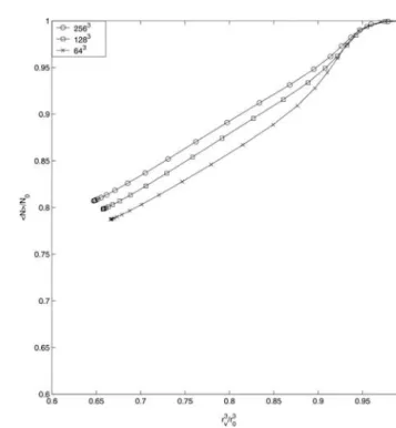
Figure 3 shows the evolution of cloud droplets num-ber,N, plotted as a function of the mean volume radius cubed,r3
, scaled by their initial valuesN0and r0, for
the three simulations in set S1b. This diagram will be referred to as ther⫺Ndiagram throughout the rest of this paper. It was adopted in AGMS after Brenguier and Burnet (1996); see also Chosson et al. (2004) and Burnet and Brenguier (2007, hereafter BB). In AGMS (their Fig. 13), only (r/r0)
3
andN/N0of the final
mix-ture were shown, whereas figures herein document the entire evolution of the microphysical parameters, from the start of the simulations [upper-right corner; (1, 1)] toward the completion of the mixing around (0.65, 0.80).
In ther⫺Ndiagram, the final states of all possible microphysical realizations, for given initial conditions, reside on the hyperbola implied byNr3
⫽ N0r 3
0 ⫽
const (Fig. 13 in AGMS), where, the ratio of the mean cloud water after and before the mixing, is given by the FIG. 2. Evolution of the TKE dissipation in the low-TKE input
simulations applying detailed microphysics: set S1b. The solid lines are the theoretical predictions based on the enstrophy evo-lution, whereas the dashed line is the dissipation diagnosed from the TKE evolution and the buoyancy production term.
FIG. 1. Evolution of the TKE in simulations with the low-TKE input and with bulk (solid line) and detailed (dashed line) repre-sentations of the cloud microphysics: sets S1a and S1b. Results from simulations applying grid sizes of (top) 2563, (middle) 1283,
and (bottom) 643.
FIG. 3. Results from the detailed microphysics simulations with low-TKE input applying grid sizes of 2563, 1283, and 643(set S1b)
plotted in ther⫺Ndiagram. The symbols along the lines are plotted every 0.8 s to demonstrate the elapsed time, from the starting point (upper-right corner) toward the lower left.
bulk thermodynamic properties of cloudy and cloud-free air andX(cf. section 5 in AGMS for a discussion). The impacts of the two limiting conceptual models of the microscale homogenization on cloud droplet spec-tra are easily identified in ther⫺Ndiagram. The ho-mogeneous model assumes that all droplets are ex-posed to the same environmental conditions during ho-mogenization. It follows that all droplets experience some evaporation and the number of cloud droplets does not change. Consequently, homogeneous mixing is represented by a horizontal line segment from (1, 1) to (, 1). In the extremely inhomogeneous model (Baker and Latham 1979; Baker et al. 1980), on the other hand, some droplets evaporate completely whereas others do not change their sizes at all. In such a case, the number of droplets decreases, but their size remains constant. Such a change is represented by a vertical line segment from (1, 1) to (1,).
Results shown in Fig. 3 document that the mixing in the three simulations falls somewhere in between the two limiting conceptual models, and that the simulated microphysical transformations only weakly depend on the model resolution. The latter finding corroborates the validity of the results reported in AGMS, and indi-cates the adequacy of the 643 grid for the sensitivity studies discussed in subsequent sections.
To illustrate the relevance of our numerical studies to the cloud chamber experiment of Malinowski et al. (1998) and Korczyk et al. (2006)—the original motiva-tion behind this work—Fig. 4 compares a cross secmotiva-tion from the 2563 low-TKE input simulation with a laser-sheet photograph of cloudy and clear air filaments in
the laboratory experiment. The size of the two-dimensional cross section is approximately the same (about 0.6 m⫻0.6 m). The photograph from the cloud chamber shows finescale structures within cloudy fila-ments that result from the scattering of laser light by individual droplets. In contrast, the numerical model output displays only a continuous cloud water field. The resemblance of the larger-scale topological struc-tures (filaments and eddies) between the numerical model result and laboratory experiment is noteworthy.
4. Microphysical transformations during turbulent mixing: Reference study
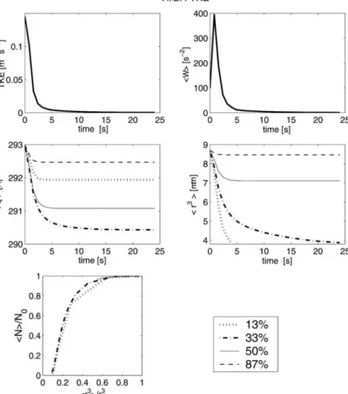
The simulations in sets S2a, S2b, and S2c of Table 2 investigate the sensitivity of microphysical transforma-tions to the TKE input and initial volume proportion of the cloudy airX. All three sets use the detailed micro-physics, 643grid, as well as fixed initial liquid water in cloudy filaments and the relative humidity of clear air. All simulations in AGMS assumed an idealized mix-ing scenario withX⫽0.5. Here, we consider a range of
X∈]0, 1[. VaryingXhas important implications for the thermodynamic state after homogenization. This is il-lustrated in Fig. 5, a mixing diagram for cloudy and clear air (cf. Grabowski 1993) with the thermodynamic initial conditions assumed. The diagram shows the den-sity temperatureT[see Emanuel 1994, Eq. (4.3.6)] af-ter homogenization as a function of X; T ⬇ T(1 ⫹
⑀q⫺qc), whereTis the air temperature,⑀ ⫹1⬅R/Rd
is the ratio of the gas constants for water vapor and dry air, andqandqcare the water vapor and cloud water
FIG. 4. (right) Vertical cross section from the 2563detailed microphysics simulation with low-TKE input att⫽
5 s and (left) a laser-sheet photograph of mixing structures observed in the laboratory. Both panels are about 0.6 m⫻0.6 m. Direction of gravity is from top to bottom.
mixing ratios. The mixing diagram consists of two line segments (theoretical predictions) whose common point (X⬇0.34,T⬇292.6 K) represents a state where the homogenized mixture is at saturation and contains no cloud water. This is the mixture with the lowest density temperature, that is, with the smallest buoyancy gT⬘/T
o (here, g is the gravitational acceleration and
the prime denotes deviations from the initial valueT
o
of the clear air, the same as in the cloudy air in the reference setup). The segment to the left of the com-mon point (X⬍0.34) corresponds to the unsaturated, cloud-free homogenized mixtures, whereas the segment to the right (X ⬎ 0.34) corresponds to the saturated cloudy mixtures. The asterisks on the segments showT of the homogenized mixture, as simulated by the model, for selected values of X, applying detailed mi-crophysics and low-TKE input.
The mixing diagram documents that the model accu-rately reproduces the bulk thermodynamic properties of the homogenized mixture.2Furthermore, the mixing diagram shows that varying X results in substantial changes toT. The estimated negative buoyancy after the homogenization ranges from about ⫺1.7 ⫻ 10⫺2 m s⫺2forX⫽0.87 to about⫺7.7⫻10⫺2m s⫺2X⫽0.33.
The impact of theseT variations on the mean buoy-ancy, and vertical velocity, has already been explained in the closing paragraph of section 2 (and the appen-dix). The impact on the microphysical transformations is discussed below.
The results from simulation sets S2a, S2b, and S2c are summarized in Figs. 6, 7, and 8, respectively, for the low-, medium-, and high-TKE inputs. The figures show the evolution of the domain-average TKE, enstrophy, temperature, and the mean volume radiusr⬅ 具r3典1/3.
Furthermore, the evolution of the cloud droplets num-berNand the mean volume radius cubedr3
are
com-bined in ther⫺Ndiagram.
For the low-TKE input (Fig. 6) most of the TKE is generated as a result of the evaporation of cloud drop-lets during the first 10 s of the simulation. The evolu-tions of the mean temperature and the mean volume radius are consistent with our expectations following the basic physics of mixing: the lowest temperature is obtained forX⫽0.33 (cf. Fig. 5) and the mean radius of the homogenized mixture decreases with diminishingX. For simulations with differentX, the maximum values of TKE are in the range from about 2⫻10⫺3to about 3⫻10⫺3 m2s⫺2, whereas the maximum values of the
mean enstrophy are from about 4 to about 8 s⫺2. These
differences are relatively small considering the differ-ences in the realizable negative buoyancy (within a fac-tor of 5; cf. Fig. 5). Moreover, the actual value of the maximum TKE (aroundt⫽ 10 s) is unrelated to the potential for buoyancy reversal. For instance, the larg-est and smalllarg-est TKE maxima are reached in simula-tions with, respectively,X⫽0.13 andX⫽0.87—the two cases with the lowest potential for the buoyancy rever-sal. The lack of correlation between TKE and the po-tential for the buoyancy reversal suggests that the in-terfacial mixing occurs locally, as a result of molecular diffusion and droplet sedimentation across the inter-face, whileX, a global measure, is of secondary impor-tance. In other words, the global mixing proportion af-fects the mean buoyancy—hence, the Lagrangian par-cel’s acceleration and mean vertical velocity, see the appendix—and not the dynamics of the small-scale tur-bulent mixing.
The most intriguing aspect is the evolution of micro-physical properties displayed in ther⫺Ndiagram. All mixing events appear to follow the same path, starting from the upper-right corner of the diagram and pro-ceeding toward the lower-left corner. This implies that the average microphysical properties are approximately the same regardless of the progress of mixing. For in-stance, the transient microphysical properties forX⫽
0.13, 0.33, and 0.43 all pass close to the final properties
2The case
X⫽0.33 has still not reached the equilibrium con-ditions. Traces of cloud water are present in the computational domain at the end of this simulation because the final point in the
r⫺Ndiagram is not at (0, 0); see Fig. 6.
FIG. 5. Density temperatureTafter homogenization as a func-tion of the initial proporfunc-tion of the cloudy air volumeXfor the reference group of model simulations (cf. Table 2). Solid lines represent theoretical predictions; the asterisks represent values calculated using final thermodynamic properties from numerical simulations with detailed microphysics and the low-TKE input (i.e., set S2a).
of the mixing event withX⫽0.50. In the vicinity of this point (in the diagram) in all transient states, the mean cloud water equals the final value for the mixing event withX ⫽0.50. This is an important finding because it implies that the mean microphysical properties, as mea-sured by the mean number of droplets and the mean volume radius, only weakly depend on the progress of mixing. This suggests that it may be possible to design a relatively simple parameterization to describe micro-physical transformations during entrainment and mix-ing, without the need to consider whether microscale homogenization is already completed or not.
The overall similarities of the TKE and microphysi-cal evolutions observed in the S2a microphysi-calculations for the
low-TKE input are reproduced in the S2b and S2c simulations with moderate- (Fig. 7) and high- (Fig. 8) TKE inputs, respectively. The paths of the TKE evolu-tions are predetermined by the input velocity perturba-tions. The differences in the individual evolutions of the TKE and enstrophy, for differentX, are relatively mi-nor, diminish with increasing TKE input, and vanish in the high-TKE input case. Furthermore, although the r ⫺ N diagrams show, consistent with the low-TKE input case, that microphysical properties depend only weakly on the progress of the mixing, there are system-atic differences between the three sets of simulations. In particular, a higher-TKE input leads to mixing that is initially more of the homogeneous type (i.e., the lines FIG. 6. Results from the set of numerical simulations with low-TKE input and detailed
microphysics applying the reference setup: set S2a. The evolution of the (top left) TKE and (top right) mean enstrophy. The evolution of the (middle left) mean temperature and (middle right) mean volume radius. (bottom left) The evolution of the microphysical properties using ther⫺Ndiagram.
tend to be horizontal) and changes toward the ex-tremely inhomogeneous mixing at later stages (i.e., the lines are not far from vertical).
5. Microphysical transformations during turbulent mixing: Sensitivity study
The simulations described in the previous section ap-ply a selected set of thermodynamic and microphysical parameters, representative of conditions in the labora-tory experiments (Malinowski et al. 1998; Banat and Malinowski 1999; Korczyk et al. 2006). Here, additional simulations are performed to shed light on the univer-sality of the derived conclusions. The sensitivity simu-lations fall into two distinct categories. The first inves-tigates the impact of bulk thermodynamic properties, such as the liquid water mixing ratio of cloudy fila-ments, the global mixing proportionX, and the initial relative humidity (RH) of the dry air. These
simula-tions form sets S3a, S4a, S4b, S4c, and S5a (cf. Table 3). The second group investigates the impact of the initial spectrum of cloud droplets on the resulting microphysi-cal transformations. These simulations are grouped into two sets, S6a and S6b, detailed in Table 4.
a. Impact of initial bulk thermodynamic properties In the first set of simulations, S3a, the initial liquid water within the cloudy filaments is systematically var-ied, from 0.2 to 3.2 g kg⫺1. The amount of liquid water in the cloudy filaments changes the bulk mixing dia-gram shown previously in Fig. 5. In general, decreasing the liquid water mixing ratio increases the mixing pro-portion X that corresponds to the saturated mixture (i.e., the intersection of the two line segments in Fig. 5) and increases the minimum buoyancy. The mixing pro-portions corresponding to the saturated mixtures are
X⫽0.34, 0.52, 0.77, and 0.88 for cloud water equal to, respectively, 3.2, 1.5, 0.5, and 0.2 g kg⫺1. The minimum
buoyancies are⫺7.7⫻10⫺2,⫺4.5⫻10⫺2, and⫺0.6⫻
10⫺2 m s⫺2for cloud water equal to, respectively, 3.2,
1.5, and 0.5 g kg⫺1. There is no buoyancy reversal for a cloud water mixing ratio of 0.2 g kg⫺1because the
satu-rated mixture is positively buoyant, with a buoyancy of 1.4⫻10⫺2m s⫺2, which is about half of the buoyancy of the cloudy air. The assumed range of the initial liquid water aims at representing conditions ranging from cu-mulus (the high end of the liquid water) to stratocumu-lus (the low end).
Figure 9 documents the results of simulations with thermodynamic properties as in simulations described in the previous section and X⫽ 0.5, but with system-atically varied liquid water within cloudy filaments, from 0.2 to 3.2 g kg⫺1(set S3a). Because
X⫽0.5, only the highest initial liquid water mixing ratio (3.2 g kg⫺1)
leads to the homogenized mixture with some conden-sate; all other cases result in subsaturated mixtures
without any liquid water.3 As Fig. 9 shows, in
agree-ment with results discussed in the preceding section, the resulting maximum TKE varies within a factor of 2 be-tween all simulations, and the evolution on ther⫺N diagram follows a similar path to the results shown in Fig. 6 (i.e., close to the lower left-upper right diagonal of the diagram).
The next three figures document the impact of vary-ing mixvary-ing proportionsXon mixing characteristics with various initial liquid water mixing ratios within the cloudy filaments; see sets S4a, S4b, and S4c in Table 3. Except for the initial liquid water, the simulations are otherwise identical to those shown in Fig. 6. Figures 10,
3The case with a 1.5 g kg⫺1initial cloud water mixing ratio
results in a mixture practically at saturation; note that this simu-lation has still not reached the equilibrium conditions because the final point in ther⫺Ndiagram is not at (0, 0).
11, and 12 document the results from simulations with initial liquid water mixing ratios of 1.5, 0.5, and 0.2 g kg⫺1, respectively. As discussed above, reducing the initial liquid water within cloudy filaments reduces the
potential for buoyancy reversal and consequently leads to a systematic decrease of the TKE levels in simula-tions with decreasing initial cloud water. Similar to the reference study simulations, the maximum TKE for a FIG. 9. Results from the set of numerical simulations with low TKE, detailed microphysics,
X⫽0.5, and systematically varied cloud water mixing ratio within cloudy filaments: set S3a. The evolutions of the (left) TKE and (right)r⫺Ndiagram.
FIG. 10. Results from the set of numerical simulations with low TKE, detailed microphysics, cloud water mixing ratio within cloudy filaments of 1.5 g kg⫺1, and systematically varied global mixing proportionX: set S4a. The evolutions of the (left) TKE and (right)r⫺Ndiagram.
given initial liquid water mixing ratio appears uncorre-lated with the global mixing proportionX. Again, as in previous cases with the low-TKE input, the results fol-low a similar path in ther⫺Ndiagram, from the upper right toward the lower left.
The last set of simulations investigating the impact of thermodynamic properties considers systematic changes of the RH within clear air filaments, with the cloud water of cloudy filaments equal to 3.2 g kg⫺1, low input TKE, and the global mixing proportionX⫽0.5 FIG. 11. As in Fig. 10 but for cloud water mixing ratio within cloudy filaments of 0.5
g kg⫺1: set S4b.
FIG. 12. As in Fig. 10 but for cloud water mixing ratio within cloudy filaments of 0.2 g kg⫺1: set S4c.
(set S5a in Table 3). The range of RH considered in this set is from 30% to 90%. The mixing diagrams for these conditions are characterized by shifting the mixing pro-portion corresponding to the minimum buoyancy from
X⫽0.52 for RH⫽30% toX⫽0.13 for RH⫽90%. It follows that for the assumed mixing proportionX⫽0.5, all but the RH ⫽ 30% simulation lead to saturated cloudy mixtures after homogenization. However, since the RH⫽30% simulation has not reached the equilib-rium conditions, the final point in ther⫺Ndiagram is not at (0, 0). The resulting liquid water mixing ratio ranges from about 0.4 g kg⫺1for RH⫽45% to about
1.5 g kg⫺1for RH⫽90%.
The results of simulations with variable RH are summarized in Fig. 13. The RH of clear air filaments has two distinct effects. First, RH affects the amount of cloud water that has to evaporate during homog-enization as discussed above. This impacts both the amount of liquid water left at the end of simulations and the negative buoyancy generated during mixing. The decreasing amount of liquid water with the de-creasing RH is demonstrated by the length of the mixing lines in the r ⫺ N diagram for the fixed global mixing proportion of 0.5 (note that the RH ⫽ 30% simulation is terminated before the equilibrium conditions are reached). Changes of the negative
buoy-ancy, on the other hand, affect the maximum TKE generated during mixing. The maximum TKE mono-tonically increases with decreasing RH, with the TKE for RH of 30% approximately three times higher than for RH of 90%. Second, the RH affects the rate of evaporation of cloud droplets that fall across the cloud– clear air interface into the subsaturated air. As a result, the RH of clear air filaments impacts the homogeneity of mixing, with high RH implying more homogeneous mixing because the homogeneous mixing is anticipated when droplet evaporation time is much longer than the time of turbulent homogenization (Baker and Latham 1979; Baker et al. 1980).4 This is evident in ther⫺N
diagram shown in Fig. 13, which documents that it is no longer true that mixing histories are close to the diagonal of ther⫺Ndiagram, especially for high RH of clear filaments. However, the departures from the diagonal are relatively minor compared to the scat-ter of curves in Figs. 6–12, especially for lower values of RH.
4It has to be pointed out, however, that the distinction between
the homogeneous and extremely inhomogeneous mixing vanishes once the relative humidity of clear air is 100% because no droplet evaporation is needed.
FIG. 13. Results from the set of numerical simulations with low TKE, detailed microphysics, cloud water mixing ratio within cloudy filaments of 3.2 g kg⫺1,X⫽0.5, and systematically varied relative humidity within clear air filaments: set S5a. The evolutions of the (left) TKE and (right)r⫺Ndiagram. The symbols along the lines are plotted every 1.6 s to demonstrate the elapsed time.
b. Impact of initial cloud microphysical properties The final two sets of model simulations, S6a and S6b in Table 4, investigate the impact of the initial cloud droplet spectrum on the microphysical transformations. In general, the initial spectrum of cloud droplets is an-ticipated to play a role via two separate mechanisms. First, larger cloud droplets fall faster across the cloud– clear air interface and may result in a different evolu-tion of the TKE and different spectral changes during homogenization. Second, larger cloud droplets require more time to evaporate (for the same ambient condi-tions) and, thus, can shift the mixing scenario toward more homogeneous mixing. It follows that increasing the droplet size for the same TKE input and the same properties of the clear air should result in more homo-geneous mixing. To show that such elementary consid-erations do provide useful insights, the final two sets of model simulations are performed (S6a and S6b) in the setup corresponding to the low-TKE input, 3.2 g kg⫺1 of cloud water within initial cloudy filaments, RH of cloud-free filaments of 30%, andX⫽0.5.
To focus the investigation (of the impact of the initial cloud droplet spectrum on the microphysical transfor-mations), we adopt an idealized approach, where the initial spectrum of cloud droplets remains fixed, but the sedimentation rate of droplets and their evaporation
rate, both depending on the droplet size, are varied separately. Technically, this is achieved by including factors ␦ and ␥ (constant for each simulation) in the formulas for droplet terminal velocity and droplet evaporation rate, respectively. For instance, by assum-ing that the sedimentation ratetis four times the
origi-nal value (given by Stokes’s law) and the evaporation rate dr/dt is half of the original value (for the same ambient conditions), the results mimic conditions with two times larger initial cloud droplets. The advantage of such an approach is that it emphasizes relevant physical mechanisms through which the initial droplet spectrum affects the mixing and homogenization.
Figure 14 shows results from set S6a of simulations where droplet terminal velocity is multiplied by a factor varying from 0 (i.e., no sedimentation) to 4. Arguably, such a spread covers the expected range of droplet sizes in natural clouds. As the figure shows, increasing the sedimentation rate increases the maximum TKE during mixing. This is consistent with the expectation that more rapid transport of cloud droplets across the cloud–clear air interface should result in enhanced negative buoyancy, and consequently more buoyantly produced TKE. The impact on the microphysical trans-formations, on the other hand, is rather small as docu-mented by ther⫺Ndiagram.
FIG. 14. Results from the set of numerical simulations with low TKE, detailed microphysics, cloud water mixing ratio within cloudy filaments of 3.2 g kg⫺1, RH within clear air filaments of 30%,X⫽0.5, and systematically varied sedimentation rate of cloud droplets: set S6a. The evolutions of the (left) TKE and (right)r⫺Ndiagram.
In contrast, the rate of droplet evaporation affects mostly microphysical transformations. This is docu-mented in Fig. 15, which shows the results of a series of simulations from set S6b, where the droplet growth rate dr/dtis multiplied by a factor (constant in each simula-tion) ranging from 0.125 to 8. Such a range exceeds the range of droplet sizes anticipated in natural clouds be-cause it corresponds to droplets with radii 8 times larger and 8 times smaller than in the standard setup. In fact, considering that the initial cloud droplet spectrum in the reference setup has continental characteristics (i.e., the mean droplet radius is around 9m), model results related to natural clouds would fall within the limits given by the simulations with the factors of 0.25 and 1. As Fig. 15 documents, the impact of such changes on the TKE is rather small (especially when compared to the impact through the terminal velocity), but the char-acter of the mixing is significantly affected. In agree-ment with the discussion toward the end of the previous section (i.e., the impact of clear air RH), larger droplets (i.e., droplets with longer evaporation time) result in mixing that is initially more homogeneous (i.e., the tra-jectory in ther⫺Ndiagram lies above the diagonal). Smaller droplets, on the other hand, featuring shorter evaporation time, lead to initially more inhomogeneous mixing.
In summary, as far as the microphysical transforma-tions during entrainment and mixing are concerned, the
initial cloud droplet spectrum seems to mostly affect the rate of droplet evaporation (i.e., larger droplets re-quiring more time to evaporate), whereas droplet sedi-mentation mostly affects TKE generated during mix-ing, with higher TKE present in simulations with larger droplets. These results imply that, in otherwise identical situations, larger cloud droplets lead to a more homo-geneous mixing through the combination of their ability to generate more TKE via enhanced sedimentation and their longer lifetime.
6. Discussion
For decades, entrainment and mixing have been pos-tulated as crucial processes affecting the spectrum of cloud droplets (cf. Lasher-Trapp et al. 2005; BB, and references therein). The homogeneous and extremely inhomogeneous mixing models represent two limits of admissible microphysical transformations during a mix-ing event with prescribed bulk properties of the two air parcels. As illustrated by results discussed in AGMS and in this paper, the final state of the homogenized mixture has microphysical properties somewhere be-tween the two limiting cases, with both the number of droplets and the mean droplet size modified. Since typi-cally a considerable fraction of the volume of a cumulus or stratocumulus cloud is diluted by entrainment (e.g., Blyth 1993; Wang and Albrecht 1994; Moeng 2000), FIG. 15. As in Fig. 14 but with systematically varied evaporation rate of cloud droplets: set
S6b. The circles along the lines in ther⫺Ndiagram represent the elapsed time, with each circle plotted every 1.6 s.
microphysical transformations during small-scale tur-bulent mixing are important for warm rain develop-ment (e.g., Lasher-Trapp et al. 2005) and radiative transfer through the cloudy atmosphere (Chosson et al. 2004; Grabowski 2006).
Lasher-Trapp et al. (2005) investigated the impact of entrainment on the broadening of cloud droplet spec-tra, and the role of varying supersaturation histories during parcel ascent toward the observation point (Cooper 1989). Their results corroborate the concept of the entrainment leading to the development of a sec-ondary mode, in addition to the mode produced by the adiabatic ascent from the cloud base (cf. Paluch and Knight 1984; Brenguier and Grabowski 1993). The rela-tive magnitudes of the two modes, however, appeared to be sensitive to the assumed mixing scenario— homogeneous versus extremely inhomogeneous—with realistic droplet spectra produced in simulations blend-ing the two limits.
Chosson et al. (2004) documented the impact of the mixing assumption on the radiative transfer by per-forming LESs of a stratoculumulus cloud and applying the results to a radiation transfer model. Because the radiation model requires cloud droplet size distribu-tion, information that is unavailable from the bulk model, the following approach was used. In undiluted (adiabatic) cloud volumes, droplet size distributions were calculated using an adiabatic growth model and the observed droplet spectrum near the cloud base. In the diluted volumes, on the other hand, the homoge-neous and extremely inhomogehomoge-neous mixing scenarios were separately considered and the sensitivity to these two extreme limits was investigated. The results turned out to be surprisingly sensitive to the assumed mixing scenario, with the cloud optical depth about 35% larger for the homogeneous mixing than for the extremely inhomogeneous mixing scenario. This was argued to have far-reaching consequences for satellite remote sensing of clouds.
A similar investigation for the case of cumulus con-vection was reported in Grabowski (2006). Therein, it was shown that varying the assumptions concerning the homogeneity of mixing in diluted volumes of convec-tive clouds had a major impact on the amount of solar energy reaching the surface. In particular, the first in-direct effect of atmospheric aerosols, the so-called Twomey effect (Twomey 1974, 1977), turned out to be the same in either clean clouds assuming the homoge-neous mixing or polluted clouds with the extremely in-homogeneous mixing.
To assess meteorological implications of our results, we attempt to relate model results to cloud
observa-tions. Ther⫺Ndiagram adopted throughout this pa-per uses the total number of droplets involved in the mixing event as one of the variables—a natural choice in reductionistic model simulations. However, it can be easily converted into the Brenguier and Burnet (1996) diagram that uses measured droplet concentration; see also Chosson et al. (2004) and BB. This is demonstrated in Fig. 16, where ther⫺Ndiagram shown in Fig. 6 is transformed such that the vertical axis is the concentra-tionC, that is, the number of dropletsNdivided by the volume of the computational domain (ther⫺C dia-gram). Because the adiabatic concentration Co
corre-sponds to the situation where the entire computational domain is filled with the initial cloudy air, the starting points for lines representing simulations with different mixing proportionsXare no longer at the upper-right corner, that is, at (1, 1). Instead, the starting point for each simulation in the r⫺ C diagram represents the initial mixing proportion; that is, it is located at (1,X). Moreover, because the total number of droplets does not change during homogeneous mixing (unless all droplets evaporate), paths that correspond to the ho-mogeneous mixing are horizontal lines connecting the starting point (1,X) with the nondimensional mean vol-ume radius determined by the bulk mixing characteris-tics (i.e., the cloud water left after homogenization). Clearly, representing the mixing in ther⫺Cdiagram obscures the similarity of solutions obtained with vari-ous mixing proportions in ther⫺Ndiagram.
Converting aircraft observations to the format of the r⫺Ndiagram is not an easy task. First, the limitations of the aircraft instrumentation need to be recognized. FIG. 16. Ther⫺Cdiagram from the set of simulations shown in Fig. 6. The circles show the ending points of the horizontal trajectories, which represent homogeneous mixing given the ini-tial mixing proportionX⫽C/Co.
The entrainment and mixing between a cloud and its clear environment are often envisioned as a two-stage process, where the initial stirring produces filaments of cloudy and clear air, and molecular mixing across the interface separating the filaments completes the mi-croscale homogenization (e.g., Broadwell and Brei-denthal 1982; Jensen and Baker 1989; Malinowski and Zawadzki 1993). When analyzing data from an aircraft flying through a volume still in the first stage of mixing, results obtained with instruments not capable of resolv-ing microscale structures can easily be interpreted as representing extremely inhomogeneous mixing (see a discussion in section 5 of Paluch and Baumgardner 1989). This purely instrumental effect results in an ap-parent dilution of cloud droplets, as illustrated by the starting points of the trajectories in ther⫺Cdiagram in Fig. 16. Moreover, a “mixing event,” where a given mass of cloudy air initiates and completes mixing with a given mass of clear air, is difficult to observe in natural clouds.
One can attempt, nevertheless, to convert aircraft ob-servations into ther⫺Ndiagram applying the follow-ing strategy. First, one has to assume that cloud dilution observed at a given level results from a single mixing event between undiluted cloudy air at this level and subsaturated environmental air at the same level. This assumption is likely often violated in clouds because of a possibility of multiple mixing events and of the ver-tical displacement of a parcel undergoing mixing. It does, however, allow for a straightforward conversion of cloud observations into ther⫺Ndiagram. The pro-cedure is to first use the observed total water (the sum of the water vapor and cloud water mixing ratios, which is invariant when there is no precipitation) to derive the mixing proportion between the undiluted cloudy air and subsaturated environmental air at the same level. Multiplying the mixing proportion by the undiluted droplet concentration (estimated from the area of the cloud that is as close to adiabatic as possible) gives an estimate of the number of droplets (per unit volume) involved in the mixing event. This number, together with the mean volume radius of the undiluted cloudy air, are then used to normalize the observed local con-centration and the local mean volume radius. The result of such a procedure for the Fast-Forward Scattering Spectrometer Probe (Fast-FSSP) data (Burnet and Brenguier 2002; BB) collected during one of the Météo-France Merlin IV flights during the Small Cu-mulus Microphysics Experiment (July–August 1995, in Florida) is shown in Fig. 17. The result is a large cluster of points corresponding to neither the homogeneous nor the extremely inhomogeneous mixing scenarios, which is consistent with our DNS study.
Arguably, the most significant conclusion of our study is that the average microphysical properties of the mixture only weakly depend on the macroscopic mixing proportion and on the progress of mixing. This implies that a parameterization can be developed for represent-ing the small-scale inhomogeneities and their impact on microphysical characteristics. Such a parameterization would be a DNS-derived microphysical subgrid-scale model for a dynamical LES that assumes grid-scale ho-mogenized-dependent variables. Furthermore, the re-duced parameterization would be equally relevant to models with bulk microphysics, when needed to supply microphysical parameters for radiative transfer (e.g., Chosson et al. 2004; Grabowski 2006). Our results sug-gest that it is feasible to account for departures from the homogeneity of subgrid-scale mixing in contemporary cloud models. Possible approaches will be the subject of future research.
Although our results do have potentially significant implications for the warm rain development and radia-tive transfer through warm (ice free) clouds, it is pre-mature to speculate on the specifics. This is because of the small volume considered in the simulations com-pared to the mean free path of a photon inside a cloud (typically several tens of meters or longer) and the lack of vertical motion of the parcel during mixing and ho-FIG. 17. Ther⫺Ndiagram for cloud penetrations near the top of cumulus clusters at an altitude of about 2400 m during the 5 August flight of the Météo-France Merlin IV (from 1402:30 to 1514:00 UTC) during the Small Cumulus Microphysics (SCMS) experiment. Each point corresponds to observed cloud droplet properties converted to the number of droplets involved in a single mixing event.
mogenization, which may provide fresh nucleation and/ or “superadiabatic” growth of some droplets. These is-sues will be addressed in future studies where a subgrid-scale parameterization developed using the current results is applied in LES simulations of warm clouds. Work in this area has already begun and modeling re-sults will be reported upon as they become available.
7. Summary
The reported computational study of decaying moist turbulence extends the calculations of AGMS. Inspired by laboratory experiments (Malinowski et al. 1998; Korczyk et al. 2006), the adopted modeling setup fol-lows the DNS of dry transient isotropic homogeneous turbulence (Herring and Kerr 1993), in an attempt to bridge the gap between laboratory experiments and natural clouds. The emphasis is on the final stage of the entrainment and mixing, when the filamentation by large-scale eddies is already completed and mixing/ evaporative cooling takes place (Jensen and Baker 1989). The present work examines the accuracy of the AGMS results obtained at relatively coarse spatial resolution and the sensitivity of solutions to the initial thermodynamic properties of cloudy and clear air, mix-ing proportions, and microphysical properties of cloud droplets.
The first issue is resolved by means of a convergence study for the fixed initial conditions and physical do-main. The analysis of a series of simulations with 643,
1283, and 2563grid points demonstrates that at the
high-est resolution (⌬x⫽0.25⫻10⫺2m) calculations resolve
the molecular dissipation, that is, fall into the DNS re-gime. The DNS experiments accurately represent physical processes from O(1 m) down to the Kolmo-gorov scale. Most importantly, the integral characteris-tics of the DNS results match the results of coarser-grid simulations, both here and in AGMS, including turbu-lence evolution as well as the turbuturbu-lence effect on cloud microphysics. The implications of this finding are two-fold. First, this corroborates earlier results (Doma-radzki et al. 2003; Margolin et al. 1999, 2002, 2006; and references therein) on implicit LESs ofdryturbulence with a subgrid-scale model supplied by effective nu-merical viscosity. Second, it enables extensive paramet-ric studies of cloud–clear air mixing at affordable reso-lutions.
Several sets of detailed microphysics simulations are performed at the low spatial resolution. First, the role of the initial volume proportion Xin turbulent mixing and homogenization is investigated using low-, moder-ate-, and high-TKE inputs and thermodynamic
param-eters as in AGMS. The parameter Xstrongly impacts the buoyancy of the homogenized volume (Fig. 5), but its effect on the turbulence appears small. This is true even for the low-TKE input, where most of the TKE is produced buoyantly, stemming from droplet evapora-tion near the cloud–clear air interface. This result shows that local buoyancy reversal and microscale dy-namics are independent of the global mixing propor-tion. In contrast, the mean vertical velocity is forced by the mean buoyancy, via (A4), and thus depends onX. The set of detailed microphysics simulations with variableX and variable input TKE demonstrates that the evolution of microphysical properties in ther⫺N diagram (adapted from Brenguier and Burnet 1996) follows a universal path that depends primarily on the initial TKE input. For the low-TKE input, the path of microphysical transformations is along the diagonal in ther⫺Ndiagram, reflecting equal changes of the di-mensionless droplet number and the mean volume ra-dius cubed during the homogenization. For higher-input TKE, the mixing is more complicated. In early stages, mixing shifts toward the homogeneous mixing, corroborating the classical argument based on scale analysis (Baker and Latham 1979; Baker et al. 1980; Jensen and Baker 1989). At later stages, when most of the TKE is already dissipated, the mixing resembles the extremely inhomogeneous type. The similarity of the mixing evolution in ther⫺Ndiagram (i.e., the lack of dependence onX) paves the way to subgrid-scale mi-crophysics models that account for cloud dilution due to entrainment.
In subsequent sensitivity simulations using the low-TKE input, the impact of thermodynamic and micro-physical properties of cloudy and clear air on mixing characteristics is studied. The initial cloud water within cloudy filaments has a small impact, with microphysical transformations for low-TKE input again close to the diagonal in ther⫺Ndiagram. The relative humidity (RH) of clear air filaments turns out to be more impor-tant, with higher RH resulting in a more homogeneous mixing and microphysical transformations deviating from the diagonal in ther⫺Ndiagram. This is consis-tent with the fact that high RH increases droplet evapo-ration time. An additional shift toward the homoge-neous mixing can be provided by assuming larger cloud droplets, featuring longer evaporation time and allow-ing for more TKE generation.
Finally, there are processes neglected in the present study that may play a role in natural clouds. First, the dynamics of cloud droplet motion is simplified by ne-glecting droplet inertia, a resultant of gravity and drag. According to the calculations of Bajer et al. (2000),
Vaillancourt et al. (2002), and Falkovich and Pumir (2004), the inertial effects can influence the local con-centration of cloud droplets even in a homogeneous cloud. Although the quantitative estimates are uncer-tain (see Grabowski and Vaillancourt 1999 for a discus-sion), recent experimental results show fluctuations of the local concentration of droplets of the order of a few percent (Jaczewski and Malinowski 2005), which are most likely insignificant for the processes investigated herein. Second, for the problem at hand, a continuous model for representing the discrete cloud water phase becomes questionable at the DNS resolution ⌬x ⫽ 2.5⫻10⫺3m, which is already on the order of the mean
distance between cloud dropletsO(10⫺3m). An
alter-native multiphase system approach that accounts for individual droplet dynamics and evaporation (Vaillan-court et al. 2002) might be considered in future studies to address such outstanding issues. Finally, fresh nucle-ation of cloud droplets due to entrainment has no im-pact on the spectrum of cloud droplets in the current simulations. In reality, however, fresh nucleation is an-ticipated (cf. Paluch and Knight 1984; Brenguier and Grabowski 1993; Su et al. 1998; Lasher-Trapp et al. 2005). Our interpretation of previous results is that fresh nucleation happens when a cloudy parcel under-going mixing with its subsaturated environment contin-ues to rise. This effect, neglected in the current study, should be investigated in the future as well. One pos-sibility is to use the same modeling setup, but allowing for a gradual change of the ambient pressure as the mixing and homogenization progresses. This may bring some parts of the computational domain to saturation and allow nucleation of new cloud droplets. All of the above factors warrant further numerical studies.
Acknowledgments.This work was supported by the European Commission Fifth Framework Program’s Project EVK2-CT2002-80010-CESSAR, by NCAR’s Clouds in Climate and Geophysical Turbulence Pro-grams, by the Department of Energy’s (DOE) Climate Change Prediction Program (CCPP), by Los Alamos National Laboratory’s Directed Research and Devel-opment Project “Resolving the Aerosol Climate Water Puzzle (20050014DR),” and by NOAA Grant NA05OAR4310107. The computations were per-formed at the Interdisciplinary Center for Mathemati-cal and Computational Modeling of Warsaw University and at NCAR. Comments on earlier versions of this manuscript by Jean-Louis Brenguier, Steve Krueger, and Raymond Shaw are gratefully acknowledged. We thank Jean-Louis Brenguier and Fred Burnet for pro-viding us the aircraft data used in Fig. 17. NCAR is sponsored by the National Science Foundation.
APPENDIX Mean Buoyancy Removal
The momentum and mass continuity equations for the incompressible Boussinesq fluid can be written compactly as follows: ⭸v ⭸t⫹v·v⫽ ⫺⫹kB⫹ⵜ 2 v, 共A1兲 ·v⫽0, 共A2兲
where v ⫽ (u, , w) is the velocity vector, is the pressure perturbation normalized by the reference den-sity,k ⫽(0, 0, 1) is the unit vector in the vertical, B denotes the buoyancy, andis the kinematic viscosity. With periodic boundary conditions and the generation of domain-averaged buoyancy (due to the evaporation of cloud droplets), the mean vertical velocity develops during the course of the simulations. In particular, in-tegrating (A2) over the fixed horizontal domain, ap-plying periodic boundary conditions in the horizontal, and dividing by the integration surface area results in
⭸w
⭸z ⫽0, 共A3兲
thereby implying a uniform (in the vertical) horizon-tally averaged vertical velocitywequal to the volume-averaged具w典.
Integrating the flux form of (A1) over the entire vol-ume of the domain, applying triply periodic boundary conditions, and dividing by the volume reduces (A1) to the equation governing the volume-averaged velocity:
d
dt具v典共t兲⫽k具B典共t兲. 共A4兲 Equation (A4) states that the volume-averaged hori-zontal velocities remain constant in time, whereas the volume-averaged vertical velocity responds to the evo-lution of the volume-averaged buoyancy.
Decomposing the velocity and buoyancy fields into time-dependent volume-averaged components and per-turbations
v⫽具v典⫹vⴕ, B⫽具B典⫹B⬘, 共A5兲 and inserting (A5) into (A1), while using (A4), results in the equivalent, perturbation form of (A1):
⭸vⴕ
⭸t ⫹vⴕ·vⴕ⫽ ⫺⫹kB⬘⫹ⵜ
2
vⴕ⫺具v典·vⴕ.