NBER WORKING PAPER SERIES
TECHNOLOGICAL REVOLUTIONS AND STOCK PRICES Lubos Pastor
Pietro Veronesi Working Paper 11876
http://www.nber.org/papers/w11876
NATIONAL BUREAU OF ECONOMIC RESEARCH 1050 Massachusetts Avenue
Cambridge, MA 02138 December 2005 Revised February 2008
We thank Sreedhar Bharath, Markus Brunnermeier, Leonid Kogan, Lars Lochstoer, Lu Zhang, and
especially Judy Chevalier and two anonymous referees for very helpful comments. We also thank
Malcolm Baker, Robert Barro, Efraim Benmelech, Gene Fama, Bob Fogel, Boyan Jovanovic, John
Heaton, Ali Lazrak, Robert Novy-Marx, Rob Stambaugh, Dmitriy Stolyarov, and the audiences at
the 2008 AEA meeting, 2007 AFA meeting, 2006 EFA meeting, 2006 UBC Summer Conference,
Fall 2005 NBER Asset Pricing meeting, CERGE-EI Prague, Dartmouth College, Ente Einaudi, Harvard
University, Indiana University, London Business School, London School of Economics, New York
University, Stockholm Institute for Financial Re- search, Stockholm School of Economics, University
of Chicago, University of Pennsylvania, and University of Vienna. Shastri Sandy has provided valuable
research assistance. The views expressed herein are those of the author(s) and do not necessarily reflect
the views of the National Bureau of Economic Research.
© 2005 by Lubos Pastor and Pietro Veronesi. All rights reserved. Short sections of text, not to exceed
two paragraphs, may be quoted without explicit permission provided that full credit, including © notice,
Technological Revolutions and Stock Prices Lubos Pastor and Pietro Veronesi
NBER Working Paper No. 11876 December 2005, Revised February 2008
JEL No. G1
ABSTRACT
We develop a general equilibrium model in which stock prices of innovative firms exhibit "bubbles" during technological revolutions. In the model, the average productivity of a new technology is uncertain and subject to learning. During technological revolutions, the nature of this uncertainty changes from idiosyncratic to systematic. The resulting "bubbles" in stock prices are observable ex post but unpredictable ex ante, and they are most pronounced for technologies characterized by high uncertainty and fast adoption. We find empirical support for the model’s predictions in 1830-1861 and 1992-2005 when the railroad and Internet technologies spread in the United States.
Lubos Pastor
Graduate School of Business University of Chicago 5807 South Woodlawn Ave Chicago, IL 60637
and NBER
lubos.pastor@chicagogsb.edu Pietro Veronesi
Graduate School of Business University of Chicago
5807 South Woodlawn Avenue Chicago, IL 60637
and NBER
“Technological revolutions and financial bubbles seem to go hand in hand.” The Economist, Sep 21, 2000.
1.
Introduction
Technological revolutions tend to be accompanied by bubble-like patterns in the stock prices of firms that employ the new technology. After an initial surge, stock prices of innovative firms usually fall in the presence of high volatility. Recent examples of such price patterns include the “Internet craze” of the late 1990s, the “biotech revolution” of the early 1980s, and the “tronics boom” of the early 1960s, as characterized by Malkiel (1999).1 Other examples
include the 1920s and the turn of the 20th century; in both periods, technological innovation spread rapidly while the stock market boomed and then faltered (e.g., Shiller, 2000).2
The bubble-like stock price behavior during technological revolutions is frequently at-tributed to market irrationality (e.g., Shiller, 2000, Perez, 2002). We propose another pos-sible explanation that does not involve irrationality. We argue that new technologies are characterized by high uncertainty about their future productivity, and that the time-varying nature of this uncertainty can also produce the observed stock price patterns.
We build a general equilibrium model of a finite-horizon representative-agent economy with two sectors: the “new economy” and the “old economy.” The old economy implements the existing technologies in large-scale production whose output determines the representa-tive agent’s wealth. The new economy, which is created when a new technology is invented, implements the new technology in small-scale production that does not affect the agent’s wealth. It is optimal for the new technology to be initially employed on a small scale because its future productivity is uncertain. By observing the new economy, the representative agent learns about the average productivity of the new technology before deciding whether to adopt the technology on a large scale. We show that this irreversible adoption takes place if the agent learns that the new technology is sufficiently productive. We define a technological revolution as a period concluded by a large-scale adoption of a new technology.
We show that the nature of the risk associated with new technologies changes over time. Initially, this risk is mostly idiosyncratic due to the small scale of production and a low probability of a large-scale adoption. The risk remains idiosyncratic for those technologies
1
According to Malkiel (1999), “What electronics was to the 1960s, biotechnology became to the 1980s... Valuation levels of biotechnology stocks reached levels previously unknown to investors... From the mid-1980s to the late 1980s, most biotechnology stocks lost three-quarters of their market value.”
2
“Every previous technological revolution has created a speculative bubble... With each wave of technol-ogy, share prices soared and later fell... The inventions of the late 19th century drove p-e ratios to a peak in 1901, the year of the first transatlantic radio transmission. By 1920 shares prices had dropped by 70% in real terms. The roaring twenties were also seen as a “new era”: share prices soared as electricity boosted efficiency and car ownership spread. After peaking in 1929, real share prices tumbled by 80% over the next three years.” (The Economist, September 21, 2000, Bubble.com)
that are never adopted on a large scale. For the technologies that are ultimately adopted, however, the risk must gradually change from idiosyncratic to systematic. As the probability of adoption increases, the new technology becomes more likely to affect the old economy and with it the representative agent’s wealth, so systematic risk in the economy increases.
This time-varying nature of risk has interesting implications for stock prices. Initially, while uncertainty about the new technology is mostly idiosyncratic, the new economy stocks command high market values. As the adoption probability increases, the resulting increase in systematic risk pushes up the discount rates and thus depresses stock prices in both the new and old economies. The new economy stock prices fall deeper because their discount rates rise higher due to an increase in the new economy’s market beta.
Stock prices are affected not only by discount rates but also by expected cash flows. The technologies that are ultimately adopted must turn out to be sufficiently productive before the adoption. This positive cash flow news pushes stock prices up, countervailing the effect of the higher discount rate. The cash flow effect prevails initially, pushing the new economy stock prices up, but the discount rate effect prevails eventually, pushing the stock prices down. The resulting pattern in the new economy stock prices looks like a bubble but it obtains under rational expectations through a general equilibrium effect.
The bubble-like pattern in stock prices arises in part due to an ex post selection bias. Researchers study technological revolutions with the ex post knowledge that the revolutions took place, but investors living through those periods did not know whether the new tech-nologies would eventually be adopted on a large scale. The representative agent in our model never expects stock prices to fall; she always expects to earn positive stock returns commen-surate to the stocks’ riskiness, and she subsequently earns those fair returns, on average. However, in those rare periods that are recognized as technological revolutions ex post, the agent’s realized returns tend to be initially positive due to good news about productivity and eventually negative due to bad news about systematic risk.
Uncertainty about new technologies affects not only the level but also the volatility of stock prices. Due to this uncertainty, the new economy stocks are more volatile than the old economy stocks. After an initial decline, the new economy’s volatility rises sharply when the stochastic discount factor becomes more volatile as a result of a higher probability of a large-scale adoption. The same effect also pushes up the new economy’s market beta and the old economy’s volatility, two different aspects of systematic risk in the economy.
in stock prices should be much stronger in the new economy than in the old economy; stock prices in both economies should reach the bottom at the end of the revolution; the new economy’s market beta should increase sharply before the end of the revolution; the new economy’s volatility should also rise sharply and it should exceed the old economy’s volatility; the old economy’s volatility should rise but less than the new economy’s volatility; the new economy’s beta and both volatilities should all peak at the end of the revolution; and the old economy’s productivity should begin rising at the end of the revolution.
All of these predictions are supported by empirical evidence from the recent Internet revolution. According to the model, this revolution ended (i.e., the probability of a large-scale adoption of the Internet technology reached one) in 2002. The “bubble” pattern was much stronger in the NASDAQ index (our proxy for the new economy) than in the NYSE/AMEX index (the old economy); both stock price indexes reached the bottom in 2002; NASDAQ’s beta doubled between 1997 and 2002; NYSE/AMEX’s return volatility also doubled and NASDAQ’s volatility tripled over the same period; NASDAQ’s volatility always exceeded NYSE/AMEX’s volatility; NASDAQ’s beta and both volatilities peaked in 2002; and the productivity growth of the U.S. economy accelerated sharply after 2002.
We also examine stock prices during the first major technological revolution in the U.S. since the opening of the U.S. stock market – the introduction of steam-powered railroads. In the 1830s and 40s, there was substantial uncertainty about whether the railroad technology would be adopted on a large scale. We analyze stock prices before the Civil War, and find that they fell before and during year 1857, with railroad stocks falling more than non-railroad stocks. The non-railroad stock volatility and price-dividend ratios consistently exceeded their non-railroad counterparts. The volatility of all stocks rose in 1857. The railroad stock beta increased sharply in the 1850s, before falling right after 1857. In the context of our model, all of this evidence is consistent with a large-scale adoption of the railroad technology around 1857, soon after railroads began expanding west of the Mississippi River.
Much of the literature on technological innovation analyzes issues different from those addressed here. Unlike Romer (1990), Aghion and Howitt (1992), and others, we take tech-nological inventions to be exogenous. We do not examine the links between techtech-nological revolutions and human capital (e.g., Chari and Hopenhayn, 1991, Caselli, 1999, Manuelli, 2003). Different but related models of learning are presented in Jovanovic (1982), Jovanovic and Nyarko (1996), and Atkeson and Kehoe (2007). We empirically examine the Internet and railroad revolutions, while other technological revolutions are examined by Jovanovic and Rousseau (2003, 2005), Mazzucato (2002), and others. Mokyr (1990) argues that
tech-nological progress is discontinuous, as assumed in our model, and that occasional seminal inventions (“macroinventions”) are the key sources of economic growth.
A small but growing literature explores the links between technological innovation and stock prices (e.g., Jovanovic and MacDonald, 1994, and Laitner and Stolyarov, 2003, 2004a,b). According to Greenwood and Jovanovic (1999) and Hobijn and Jovanovic (2001), innovation causes the stock market to drop because the incumbent firms are unable or unwilling to im-plement the new technology. Similar initial stock market drops are obtained in the models of Laitner and Stolyarov (2003) and Manuelli (2003). In our model, the stock market value of the old economy also drops after the new technology is invented, mostly because of the costs and risks associated with a large-scale adoption of the new technology, but our focus is on the subsequent bubble-like stock price pattern in the new economy.
The paper is organized as follows. Section 2 presents the model. Section 3 solves for stock prices and analyzes their dynamics. Section 4 investigates the model’s empirical predictions for stock prices during technological revolutions. Section 5 empirically examines the behavior of stock prices in 1830–1861 and 1992–2005 when the railroad technology and the Internet technologies, respectively, spread in the United States. Section 6 concludes.
2.
The Economy
We consider an economy with a finite horizon [0, T]. A representative agent has preferences defined by power utility over terminal wealth WT, with risk aversionγ >1:
u(WT) = W
1−γ
T
1−γ. (1)
At time t = 0, the agent is endowed with capital B0. Subsequently, capital is invested in
a linear technology producing output (net of depreciation) at the rate of Yt = ρtBt. Since
there is no intermediate consumption, all output is reinvested, and capital Bt follows
dBt=Ytdt =ρtBtdt. (2)
Productivityρt follows a mean-reverting process whose mean is determined by the available
technology. There are two technologies: “old” and “new.” Initially, only the old technology is available, and the long-run mean of ρt is equal to ρ. At time t∗, the new technology
becomes available. If the representative agent adopts the new technology at time t∗∗
≥ t∗
, the long-run mean of ρt changes from ρ toρ+ψ. Thus, the dynamics of ρt are given by
dρt = φ(ρ−ρt)dt+σdZ0,t, 0< t < t
∗∗
(3) dρt = φ(ρ+ψ−ρt)dt+σdZ0,t, t∗∗ ≤t < T, (4)
where φ is the speed of mean reversion, ρ is the mean productivity of the old technology, ψ is the “productivity gain” brought by the new technology, and σ2 is the variance of
productivity shocks, represented by the Brownian incrementsdZ0,t. That is, the adoption of
the new technology is equivalent to a shift in the economy’s average productivity.
The representative agent chooses whether and when to adopt the new technology to max-imize utility in equation (1) under the market-clearing conditionWT =BT. In equilibrium,
the agent’s final wealth must equal the amount of capital accumulated by timeT.
Our key assumption is that the productivity gain ψ is unobservable. When the new technology appears at timet∗
,ψ is drawn from a normal distribution with known variance: ψ ∼N 0,bσt2∗
. (5)
All other parameters are known. The adoption of the new technology is irreversible and costly. Converting capital to the new technology incurs a proportional conversion costκ≥0.
The agent has three choices at timet∗
when the new technology becomes available: (i) Adopt the new technology
(ii) Begin learning about the new technology (i.e., about ψ) (iii) Discard the new technology
We show below that the agent optimally chooses option (ii), so he begins learning at timet∗
. The agent learns about ψ by “experimenting” with the new technology – i.e., by implement-ing it on a small scale. After time t∗
, the economy consists of two sectors: the small-scale “new economy,” which employs the new technology, and the large-scale “old economy,” whose productivity ρt follows equation (3). The capital BtN used in the new economy is infinitely
smaller thanBt, so the agent’s wealthWT is affected by the new technology only if this
tech-nology is adopted on a large scale (i.e., by the old economy). Denoting the new economy’s productivity by ρN
t , the processes of BtN and ρNt for t > t
∗
are given by
dBtN = ρNt BtNdt (6)
dρNt = φ ρ+ψ−ρNt dt+σN,0dZ0,t+σN,1dZ1,t, (7)
where Z1,t is a Brownian motion uncorrelated with Z0,t. The agent learns about ψ by
observing ρN
t and ρt. The learning process is characterized by Lemma A1 in the Appendix.
The posterior distribution ofψ conditional on Ft=
ρN τ , ρτ :t∗ ≤τ ≤t is normal, ψ | Ft ∼N b ψt,bσ2t ,
where the posterior meanψbtis a martingale (see equation (17)) and the posterior varianceσbt2
declines deterministically over time due to learning (see equation (18)). If the new technology is adopted at timet∗∗
, the agent continues to learn about ψ by observingρN
t andρt, but the
old economy’s productivity follows equation (4) rather than equation (3). We define a technological revolution as the period [t∗
, t∗∗
] concluded by a large-scale adoption of the new technology. We treat the invention of the new technology as given, and study the conditions under which the invention leads to a technological revolution.
2.1.
Optimal Adoption of the New Technology
The agent can adopt the new technology anytime between times t∗
and T (or never). We solve for the optimal adoption timet∗∗
numerically in Section 4.2. Until then, we focus on a simpler problem in which t∗∗
denotes an exogenously given time at which the agent decides whether or not to adopt the new technology. This simpler problem admits a closed-form solution for stock prices, which improves our understanding of the stock price dynamics. Our numerical results in Section 4.2. show that the dynamics obtained when t∗∗
is endogenously chosen are very similar to those obtained here with an exogenous t∗∗
.
The sequence of events in the model is summarized in Figure 1. We assume that if a new technology is not adopted at time t∗∗
, it continues to operate on a small scale until time T. Our history is full of examples of technologies that have not been adopted on a large scale but still survive on a small scale (e.g., direct-current electric motors, airships, etc.)
Proposition 1: It is never optimal to adopt the new technology immediately at time t∗
. Adopting the new technology is risky – it may increase or decrease average productivity, depending on the sign of ψ. The prior for ψ in equation (5) is centered at zero, making the increases and decreases in productivity equally likely as of time t∗
.3 Since the agent is risk
averse, immediate adoption of the new technology is suboptimal. This intuition is formalized in the Appendix, which shows that the adoption of the new technology at timet∗
yields lower expected utility than no adoption. Proposition 1 holds for any κ, including κ = 0, as it is driven by the increase in risk resulting from the adoption of the new technology.
Proposition 2: The new technology is adopted at time t∗∗
if and only if b ψt∗∗ ≥ψ =−log (1 −κ) A2(τ∗∗) + 1 2(γ−1)A2(τ ∗∗ )bσ2t∗∗ , (8) 3
If the prior is centered atψbt∗ 6= 0, Proposition 1 is modified so that it is not optimal to adopt the new
technology at timet∗ unlessψb
where τ∗∗
=T −t∗∗
and A2(τ) =τ −(1−exp (−φτ))/φ >0.
The new technology is adopted at time t∗∗
if the expected productivity gain, ψbt∗∗, is
positive and sufficiently large. The threshold ψ is always positive, and it increases in the conversion cost κ, uncertainty σbt∗∗, and risk aversion γ, which is intuitive. Note that the
agent makes the adoption decision without knowing the true value of ψ. Regardless of the outcome of the adoption decision, learning about ψ continues after time t∗∗
.
Proposition 3: It is optimal to begin experimenting with the new technology at time t∗
. This proposition, proved in the Appendix, shows that the agent chooses to set up the new economy to begin learning about the new technology immediately after this technology becomes available at time t∗
. The intuition is simple. Experimenting allows the agent to learn about the productivity gain ψ. If this learning leads the agent to believe at time t∗∗
thatψ is sufficiently high, then it becomes optimal to adopt the new technology (Proposition 2). Otherwise, the status quo will prevail. Since experimenting is costless and there is no downside to it, it gives the agent a valuable option for free.4
Since option value generally increases with uncertainty, high uncertainty σbt∗ makes a
new technology desirable for experimentation. If it were costly to experiment with new technologies, or if the agent had to choose from a subset of technologies at time t∗
, then the technologies with the highest bσt∗ would be selected for experimentation, ceteris paribus.
Uncertainty about productivity gains is thus a natural feature of innovative technologies.
3.
Stock Prices
The stocks of the old and new economies pay liquidating dividendsBT andBTN, respectively,
at timeT. There is also a riskless bond in zero net supply, whose yield we normalize to zero, for simplicity. Since the two shocks in the model are spanned by the two stocks, markets are complete. Standard arguments then imply that the state price density is uniquely given by
πt = 1 λEt W−γ T , (9)
whereλ is the Lagrange multiplier from the utility maximization problem of the representa-tive agent. The market values (shadow prices) of the old and new economy stocks, denoted
4
The problem we solve resembles the problem of making an irreversible marriage decision. It is generally suboptimal to marry a new acquaintance immediately because of substantial uncertainty regarding the qual-ity of the personalqual-ity match (cf. Proposition 1). Instead, it seems advisable to first develop the relationship on a small scale, by dating without any commitment (cf. Proposition 3), and then to marry if we learn that the relationship is likely to work in the long run (cf. Proposition 2).
byMt and MtN, respectively, are given by the standard pricing formulas Mt =Et πTBT πt and MtN =Et πTBTN πt . (10)
To normalize the market values, we form “market-to-book” (M/B) ratiosMt/BtandMtN/BtN.
It seems reasonable to interpret capital as the book value of equity, and this interpretation is exact for Bt and BtN in equations (2) and (6) if we also interpret output and productivity
as earnings and profitability, respectively (P´astor and Veronesi, 2003).
Let pt denote the probability at time t, t∗ ≤ t < t∗∗, that the new technology will be
adopted at timet∗∗
. Lemma A3 in the Appendix shows that pt = 1− N
ψ;ψbt,σbt2−bσt2∗∗
, whereN (·;a, s2) denotes the c.d.f. of the normal distribution with meana and variance s2.
Proposition 4: For any t∈[t∗
, t∗∗
), the state price density is given by πt=λ −1 B−γ t n (1−pt)Genot +ptGeyest o , (11) whereGeno t andGe yes
t are expectations of the marginal utility of wealth conditional on whether
or not the new technology is adopted at timet∗∗
. Both values are given in the Appendix.
Corollary 1. For any t∈[t∗
, t∗∗
), the dynamics of πt are given by
dπt πt =−γA1(τ)σdZe0,t−Sπ,tbσt2 φ σN,1 dZe1,t, (12)
where τ = T −t, A1(τ) = (1−e−φτ)/φ, Sπ,t is given in the Appendix, and so are the
orthogonalized Brownian motions (Ze0,t,Ze1,t), which capture the agent’s expectation errors.
This corollary illustrates the time-varying nature of risk during technological revolutions. When a new technology arrives at time t∗
, the adoption probability pt∗ is generally small,
which makes Sπ,t∗ small as well (pt = 0 implies Sπ,t = 0). The volatility of the stochastic
discount factor in equation (12) then depends only slightly on bσ2
t, making uncertainty about
ψmostly idiosyncratic. During a technological revolution, the adoption probability increases, which makesSπ,t larger.5 As a result, the volatility of the stochastic discount factor becomes
more closely tied to bσ2
t, making uncertainty about ψ increasingly systematic.
Proposition 5: For any t∈[t∗
, t∗∗
), the market-to-book ratios are given by Mt Bt = (1−pt)G no t +ptGyest (1−pt)Genot +ptGeyest and M N t BN t = (1−pt)K no t +ptKtyes (1−pt)Genot +ptGeyest , (13) 5
In a technological revolution, pt rises from pt∗ ≈ 0 to pt∗∗ = 1, and Sπ,t rises from Sπ,t∗ ≈ 0 to Sπ,t∗∗ =γA2(τ∗∗)>0. That is, asptincreases,Sπ,t increases from approximately zero to a positive number.
where Geno t , Ge yes t , Gnot , G yes t , Ktno, andK yes
t are given in the Appendix.
In the special case pt = 0, the market-to-book ratio of the new economy simplifies into
MN t
BN t
=eC0(τ)+A1(τ)ρNt +A2(τ)ψbt+12A2(τ)2bσt2, (14)
whereA1(τ) is defined in Corollary 1, A2(τ) in Proposition 2, and C0(τ) is in the Appendix.
Note that MN/BN increases when uncertainty about ψ, bσt2, increases. This relation, first
pointed out by P´astor and Veronesi (2003) in a simpler framework, is due to the idiosyncratic nature of uncertainty. When pt= 0, the state price density does not depend on uncertainty
about ψ, but when pt > 0, it does. When pt is sufficiently large, uncertainty is mostly
systematic, and the associated risk reverses the positive relation betweenMN/BN and bσ2
t.
The return processes for both stocks are given in Corollary A1 in the Appendix. Not surprisingly, the expected stock returns are given by the return covariances withdπt/πt, and
the return volatilities of both stocks increase with uncertaintyσb2
t.
3.1.
The Dynamics of Prices during a Technological Revolution
In a technological revolution, the adoption probability pt rises from a small value at time t∗
to the value of one at time t∗∗
. The effect of pt on stock prices is analyzed next.
Proposition 6: The new (old) economy’s M/B ratio is increasing inptif and only ifhnew >0
(hold>0), where hnew and hold are functions of ψbt given in the Appendix.
For plausible parameter values, hnew > 0 when ψbt is close to zero, but hnew < 0 when
b
ψt approaches the threshold ψ. That is, the conditionhnew >0 holds shortly after time t∗,
but it becomes violated as the adoption at timet∗∗
becomes more likely. Proposition 6 then implies that the new economy’s M/B is initially increasing but ultimately decreasing in pt
during a technological revolution. The condition hold > 0 is never satisfied for the baseline
parameter values, so the old economy’s M/B is always decreasing inpt.
While analyzing M/B as a function of pt seems informative, pt is driven primarily by
b
ψt. Stock prices depend on ψbt through two opposing effects. On one hand, an increase in
b
ψt is good news for prices because it increases expected cash flows (Et[BT] and Et
BTN
) in both economies. This cash flow effect is stronger for the new economy whose perceived productivity is immediately affected; the old economy’s productivity is not affected until time t∗∗
, if at all. On the other hand, an increase in ψbt is bad news for prices because the
systematic, thereby raising the discount rate. This discount rate effect is also stronger for the new economy because πt covaries more with ρNt than with ρt (since both πt and ρNt
correlate with revisions in ψbt but ρt does not). Moreover, the discount rate effect has a
growing impact on the new economy’s M/B because the dependence of πton revisions inψbt
increases as pt increases. For the old economy, the discount rate effect generally outweighs
the cash flow effect from the very beginning, leading to a gradual decline in M/B during a revolution. For the new economy, the cash flow effect tends to dominate at first, but the discount rate effect dominates in the end, producing a “bubble”.
Although the dependence of MN/BN on ψb
t is complicated, its key features can be
estab-lished locally at timest∗
andt∗∗
. We show below that MN/BN is increasing (decreasing) in
b
ψ around timet∗
(t∗∗
), under certain assumptions.
Proposition 7: For any t≥ t∗
there exists ¯p >0 such that ifpt<p¯then ∂(MN
t /BtN)
∂ψbt >0.
In words, if the probability of adoptionptis sufficiently small, thenMN/BN is increasing
in ψbt. When pt is close to zero, so is its sensitivity to changes in ψbt; thus an increase in ψbt
does not produce a large discount rate effect.6 The cash flow effect is large, though, because
MN/BN in equation (14) is strongly increasing inψb
t. Proposition 7 follows.
When a new technology arrives at timet∗
, its probability of eventual adoption is typically small because only a small fraction of new technologies are adopted by the whole economy. Proposition 7 then implies that, for most new technologies, the cash flow effect initially prevails over the discount rate effect and MN/BN is increasing inψb
t shortly after time t∗.
We also have some local results at time t∗∗
. Below, we compare the M/B ratio of the new economy under two scenarios: ψbt∗∗ =ψ±ε, where ε >0 is small.
Corollary 2:
(a) If ψbt∗∗ =ψ+ε, then the new technology is adopted at time t∗∗, and
MN t∗∗
BN t∗∗
=eC0(τ∗∗)+A1(τ∗∗)ρNt∗∗+A2(τ∗∗)ψbt∗∗+12A2(τ∗∗)2(1−2γ)bσ2t∗∗. (15)
(b) If ψbt∗∗ =ψ −ε, then the new technology is not adopted at time t∗∗, and
MN t∗∗ BN t∗∗ =eC0(τ∗∗)+A1(τ∗∗)ρNt∗∗+A2(τ∗∗)ψbt∗∗+12A2(τ ∗∗)2bσ2 t∗∗. (16) 6
Analogously, if a stock option is deep out of the money, a small increase in the stock price does not change the option value by much since its delta is small and the option remains deep out of the money.
The new economy’s M/B is clearly lower when the technological revolution takes place. The reason is the uncertainty termbσ2
t, whose coefficient is negative in part (a) and positive in
part (b). In part (a),σb2
t is systematic (it affectsπt), whereas in part (b), it is idiosyncratic (it
does not affect πt). Since ψbt (expected cash flow) is essentially the same in both scenarios,
the difference between M/B in parts (a) and (b) is due to the discount rate effect. This knife-edge case shows thatMN/BN is likely decreasing in ψb
t close to timet∗∗.
In summary, the cash flow effect usually dominates close to time t∗
, leading to an initial positive relation between MN/BN and ψb
t, but the discount rate effect usually dominates
close to timet∗∗
, leading to an eventual negative relation. During a technological revolution,
b
ψt generally increases, leading to a bubble-like pattern in MN/BN.
3.2.
Discussion
Corollary 2 shows that the adoption reduces the new economy’s M/B, holdingψbt constant.
Intuitively, the adoption does not bring any benefit to the new economy, which already uses the new technology. On the contrary, it increases systematic risk and thus reduces the new economy’s market value. The model features only one shareholder, the representative agent, who employs infinitely more capital in the old economy than in the new economy. This agent wants the adoption to take place because the utility gain from making the old economy more productive outweighs the negligible loss of market value in the new economy.
Analogous to Corollary 2, we can show that the old economy’s market value also decreases at timet∗∗
if the adoption takes place whenψbt∗∗is close toψ. Interestingly, the representative
agent chooses to adopt the new technology even if doing so reduces the market value of her stocks. There is a difference between maximizing utility and maximizing market value. The adoption occurs only if it increases the agent’s expected utility. This adoption changes the economic environment by installing (what the agent perceives to be) a more productive technology and by increasing expected stock returns. In this new environment, stock prices are lower (due to higher discount rates) but expected utility is higher (due to higher expected wealth). Expected utility and stock prices need not move in the same direction because stock prices are related to the agent’s marginal utility rather than to the level of utility.
We solve the social planner’s problem in which a utility-maximizing representative agent owns all output by holding the stocks of the old and new economies. When a new technology is invented, it becomes property of the social planner. The social planner finds it optimal to set up a small-scale new economy to learn about the new technology before deciding whether
to adopt this technology in the large-scale old economy. Upon adoption, there is no transfer from the old economy to the new economy because the new economy does not own the new technology (the social planner does). As an example of a new economy firm, Amazon was an early user of the Internet but it did not own the Internet technology.
As an alternative to the social planner’s problem, we analyze a competitive economy in which firms independently decide whether to adopt the new technology while maximizing their own market values. We present this alternative decentralized model in the Appendix, and find that it produces the same stock price dynamics as the social planner’s problem. The alternative model features “network externalities,” in that the average productivity of a technology increases as the fraction of firms using this technology increases. Each firm makes its own adoption decision independently, taking the decisions of all other firms as given. Adopting the same technology as other firms has two opposing effects. On one hand, it hurts the firm, because the technology adopted by all other firms carries more systematic risk. On the other hand, it benefits the firm through network externality gains. We show that it is possible to choose the magnitude of the network externality gains such that the solution is identical to that in the social planner’s problem. Specifically, the Nash equilibrium at timet∗∗
is such that all firms adopt the new technology ifψbt∗∗ ≥ψ, but none of them do
ifψbt∗∗ < ψ, analogous to our Proposition 2. As a result, all pricing formulas are the same as
in the social planner’s problem, and the same “bubbles” in stock prices obtain.
The alternative model highlights the lack of coordination among firms in a competitive economy. Although each firm maximizes its own market value, the aggregate effect of the firms’ adoptions is to reduce market values. The reason is that firms adopting the new technology do not fully internalize the resulting increases in the volatility of the stochastic discount factor. Each adopting firm imposes a negative externality on the market values of other firms by increasing systematic risk in the economy. We see that the stock price patterns obtained in our simple model with a utility-maximizing social planner hold also in a more complicated model featuring value-maximizing competitive firms.
Other ways of decentralizing the model could also lead to similar stock price dynamics. For example, suppose that firms facing different conversion costs observe signals about ψ. As ψbt rises during a technological revolution, the proportion of firms that adopt the new
technology also rises. This proportion might play the same role as the adoption probability in our model: As the proportion rises from about zero to one, the volatility of the stochastic discount factor also rises, making the uncertainty about ψ increasingly systematic.
coincide. In reality, technological advances lead to permanent increases in productivity but only temporary increases in profitability. In the long run, new technology tends to benefit workers and consumers, not producers. Therefore, we also analyze a richer model in which labor income drives a wedge between productivity and profitability.7 In this model,
productivity gains from new technology last until time T, but profitability gains last only until time t∗∗∗
< T, after which all productivity gains go to labor. Profitability affects the cash flow to stocks, whereas productivity affects the discount rates. Systematic risk depends on uncertainty about productivity because the agent’s total wealth depends on productivity. As a result, our basic mechanism is unaffected by the shorter profitability horizon. Indeed, we find that this richer model produces stock price dynamics very similar to those reported here. For the same parameter values, the bubble pattern is somewhat less pronounced, but more dramatic patterns can be easily obtained after plausible parameter changes.
4.
Empirical Implications
The purpose of this section is to analyze the model-implied paths of the key variables during technological revolutions. We simulate 50,000 samples of shocks in our economy and compute the paths of quantities such as the M/B ratios and volatilities in each simulated sample. We split the 50,000 samples into two groups, depending on whether or not the new technology is adopted at timet∗∗
, and plot the average paths of prices and volatilities across all samples within each group. Our objective is to understand how these paths differ depending on whether or not the new technology leads to a technological revolution.
Table 1 shows the parameters used in our simulations. For the productivity processes, we choose parameter values close to those estimated by P´astor and Veronesi (2006) for the dynamics of profitability. The relation between productivity and profitability in our model is explained in Section 3.2. The parameter values for the conversion cost, time horizon, risk aversion, and prior beliefs about ψ are varied later in our sensitivity analysis.
Figure 2 plots the average paths of ψbt, pt, and σπ ≡ Std(dπt/πt). Panel A shows that
the average drift in ψbt during technological revolutions is positive, due to conditioning on
the ex post event that ψbt∗∗ ≥ψ (without such conditioning, ψbt is a martingale; see equation
(17)).8 Analogously, conditional onψb
t∗∗ < ψ,ψbtin Panel B (no revolution) drifts downward.
The drift is less pronounced in Panel B than in Panel A because ψbt∗ = 0 and ψ > 0. The
7
This model is presented in the Technical Appendix, which is downloadable from the authors’ websites. 8
Brown, Goetzmann and Ross (1995) provide a mathematical proof of a related statement in their analysis of stock returns conditional on the stock’s survival through the end of the sample.
average probability of adoption, pt, drifts up in Panel C (revolution) and down in Panel D
(no revolution), as expected. The volatility of the stochastic discount factor, σπ, is almost
flat whilept is low, but it increases as pt increases (Panel E).
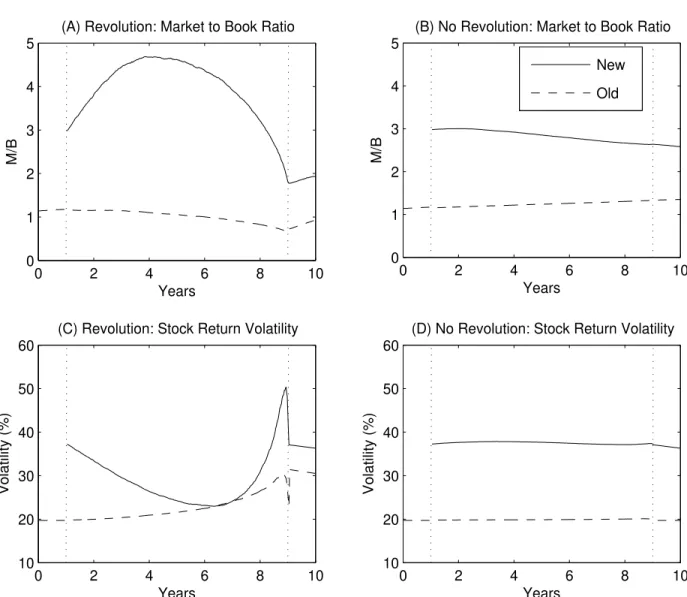
Figure 3 plots the average paths of M/B and volatility for the new economy (solid line) and the old economy (dashed line). The panels on the left are based on the samples in which pt∗∗ = 1 (revolution); the panels on the right condition on pt∗∗ = 0 (no revolution).9 The
dotted vertical lines mark the time when the new technology arrives, t∗
= 1, and the time at which the agent decides whether to adopt the technology, t∗∗
= 9.
Panel A of Figure 3 plots the average paths of M/B across all technological revolutions. The new economy’s M/B rises and then falls, as predicted in Section 3.1. Since we are conditioning on the adoption of the new technology at time t∗∗
, ψbt must go up between t∗
and t∗∗
(Figure 2). This increase in ψbt has two countervailing effects on prices. First, it
increases expected future cash flow from the new technology, pushing M/B up. Second, it increases the adoption probability, which makes the risks embedded in the new technology ever more systematic (affectingWT), which then increases the discount rate applied to future
cash flow, pushing M/B down. For the old economy, the discount rate effect outweighs the cash flow effect from the outset, leading to a slow decline in M/B. For the new economy, the cash flow effect is stronger at first, but the discount rate effect prevails in the end, producing a “bubble.” Since the path plotted in Panel A is an average across all revolutions, it shows that apparent bubbles in high-tech stock prices are not merely possible in a rational world; they should in fact be expected during technological revolutions.
Different technological revolutions produce different paths of M/B, depending on the path of realized productivity. These individual paths look mostly like bubbles that peak at different times, and they are less smooth than the average path plotted in Panel A of Figure 3. On this average path, the peak-to-bottom drop in the new economy’s M/B lasts 5 years, but for some revolutions, the price drop is much more abrupt. For example, for 10% of all revolutions, the peak-to-bottom drop lasts less than 2.56 years, and for 5% of all revolutions, it lasts less than 1.68 years. The magnitude of the price drop also exhibits substantial dispersion across revolutions. On the average path, M/B falls by 2.9 from the peak to the bottom, but for 5% of all revolutions, it falls by more than 7.8.
Panel B of Figure 3 plots the average paths of M/B across all samples in which pt∗∗ = 0
9
The fraction of the simulated samples in whichpt∗∗ = 1 is approximately equal to the ex ante probability
of adoption implied by our parameter choices,pt∗ ≈2%, as expected. In principle, any product innovation
(no revolution). In these samples,ψbtdeclines slightly between t∗ andt∗∗, nudging the M/Bs
down as well. The decline is larger in the new economy, for two reasons. One, the new economy’s M/B is more sensitive to ψbt, as discussed earlier. Two, uncertainty about ψ
gradually declines due to learning, which reduces M/B for the new economy but not for the old economy (see equation (14)). Thanks in part to this uncertainty, the level of M/B is higher in the new economy than in the old economy, in both Panels A and B. Higher productivity is another reason why the new economy’s M/B is higher in Panel A, even after time t∗∗
. Although the adoption makes the long-run means of productivity equal in both economies, the productivity at timet∗∗
is higher in the new economy (ρN
t∗∗ is likely to be high
to makeψbt∗∗ > ψ), lifting the M/B of the new economy above that of the old economy.
Panel C of Figure 3 plots the average paths of stock return volatility across all techno-logical revolutions. Volatility is higher in the new economy than in the old economy, partly due to higher volatility of the fundamentals, but mostly due to uncertainty about ψ. To understand the U-shape in the new economy’s volatility, recall that shocks to ψbt affect stock
prices via the discount rate and cash flow effects, which work in opposite directions. Around time t∗
(t∗∗
), the cash flow (discount rate) effect dominates, so the two effects do not offset each other much and the volatility is high. The volatility is lowest when the two effects cancel each other, which happens at some point between times t∗
and t∗∗
; hence the U-shape. For the old economy, the discount rate effect dominates from the outset, so the old economy’s volatility slowly increases as the rising adoption probability makes the stochastic discount factor more volatile. The spike in volatility at timet∗∗
is caused by those simulated paths for whichψbt∗∗ is close toψ because then pt swings a lot shortly before time t∗∗, making returns
highly volatile (Corollary 2). We show later that the volatility spike disappears (but all other effects remain) when t∗∗
is chosen optimally instead of being fixed exogenously. Panel D plots the average return volatility across all no-revolution samples. In these samples, the discount rate effect is weak and volatility is roughly constant over time.
Panels A and B of Figure 4 plot the market beta of the new economy, β, defined as the slope from the regression of the new economy stock returns on the old economy stock returns. In Panel A, where we condition on pt∗∗ = 1 (revolution), β exhibits an asymmetric
U-shape pattern, for the following reason. Positive shocks to ψbt always reduce the market
value of the old economy stocks, but they increase the value of the new economy stocks initially while the cash flow effect prevails over the discount rate effect, leading to an initial decrease in β. Only after the discount rate effect overcomes the cash flow effect, shocks to
b
ψt begin affecting the market values of both economies in the same direction, leading to an
probability, the rise in β is more dramatic than the initial fall. After a mild decline in the first half of the revolution,β doubles in the second half, from 0.75 to 1.5. The average beta in the no-revolution samples, plotted in Panel B, is almost flat over time.
As explained above, two aspects of systematic risk increase during technological revo-lutions: the old economy’s volatility and the new economy’s beta. The increase in the old economy’s volatility raises the discount rates for both economies, old and new, holdingβ con-stant. The increase inβ gives an additional boost to the discount rate of the new economy, which is why stock prices fall by more in the new economy than in the old economy.
The remaining panels of Figure 4 plot the average realized returns (solid line) and ex-pected returns (dashed line).10 In technological revolutions, realized stock returns are first
positive and then negative for both economies, due to an ex post selection bias. Ex post, we know that a technological revolution took place at timet∗∗
, but ex ante, we only have a probability assessment of this event. Before time t∗∗
, stock prices are not expected to rise and fall; expected returns are given simply by the covariances with the stochastic discount factor. However, conditioning on a technological revolution means that the adoption proba-bilitypt must be revised upward between timest∗ and t∗∗, causing a bubble-like pattern in
prices through the cash flow and discount rate effects discussed earlier. The bias of realized returns relative to expected returns is due solely to ex post conditioning on pt∗∗ = 1; when
this conditioning is removed, the bias disappears. (Across all 50,000 simulations, average realized returns are equal to average expected returns.) The rise and fall in stock prices during technological revolutions are observable ex post but not predictable ex ante.
The unexpected arrival of the new technology causes the old economy’s market value to drop immediately at time t∗
(Panel E of Figure 4). This drop is driven by two forces. The possibility of eventual adoption means that conversion costs might be paid at time t∗∗
, and it also increases systematic risk and so drives up the discount rate.
4.1.
Sensitivity Analysis
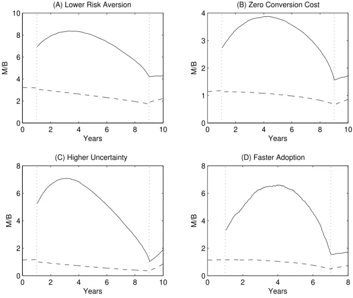
This section examines the sensitivity of the price dynamics to our parameter choices. Figure 5 is the counterpart of Panel A of Figure 3 (revolution), with various parameter changes.
In Panel A of Figure 5, risk aversionγ = 3, as opposed to γ= 4 in Figure 3. Lower risk aversion increases M/B in both economies, as expected, but the pattern of M/B is otherwise the same as that in Figure 3. A hump-shaped pattern inMN/BN obtains for any γ >1.
10
In Panel B of Figure 5, the conversion cost is κ = 0, as opposed to κ= 0.1 in Figure 3. The main effect of the lower κ is to decreaseMN/BN. The lower conversion cost makes it
more likely that the new technology will be adopted, which increases discount rates and thus depresses prices. For the old economy, there is also a counterbalancing effect, as the lower conversion cost increases the old economy’s post-conversion capitalBt∗∗
+ =Bt∗∗−(1−κ). The
two effects approximately cancel out, so the old economy’s M/B is almost unaffected by the change inκ. Most important, the price patterns look just like those in Figure 3.
In Panel C, prior uncertainty about ψ is bσt∗ = 8%, compared to bσt∗ = 4% in Figure 3.
The higher uncertainty increasesMN/BN, especially close to timet∗
whenpt is small
(equa-tion (14)). However, as pt increases during a revolution, uncertainty becomes increasingly
systematic, pushingMN/BN down, and this discount rate effect is stronger when systematic
uncertainty is higher. Therefore, in technological revolutions characterized by high uncer-tainty, the new economy firms tend to start out with high valuations that exhibit a large decline. High uncertainty amplifies the bubble-like pattern in stock prices.
In Panel D of Figure 5, the time until the adoption decision is shortened to t∗∗
−t∗
= 6, compared to t∗∗
−t∗
= 8 in Figure 3. Faster adoption increases MN/BN. To understand
this effect, we note two facts. First, faster adoption implies higher uncertainty about ψ at time t∗∗
because there is less time to learn (equation (18)). Second, faster adoption implies a higher adoption thresholdψ becauset∗∗
is lower and bσt∗∗ is higher (equation (8)). Sinceψbt
has less time to reach a higher threshold, the adoption probabilitypt∗ is lower, which implies
that systematic risk is initially lower and MN/BN starts higher than in Figure 3. MN/BN
then rises higher and falls deeper than in Figure 3, conditional on pt∗∗ = 1, because both the
cash flow effect and the discount rate effect are stronger when adoption is faster. The cash flow effect is stronger because in order for ψbt to reach a higher threshold in shorter time,
the increase in ψbt must be sharper. The discount rate effect is stronger because uncertainty
at time t∗∗
is higher, and conditional onpt∗∗ = 1, this uncertainty is systematic. Since both
effects are stronger, the rise and fall in MN/BN are more striking than in Figure 3. Faster
adoption of the new technology magnifies the bubble-like pattern in stock prices.
4.2.
Optimal Adoption Time
In this section, we relax the assumption that t∗∗
is exogenously given. Without this assump-tion, no closed-form solutions are available, but we can solve the problem numerically. The agent is choosing the optimal timet∗∗
, t∗
≤t∗∗
≤T to adopt the new technology (no adop-tion is a possibility). This is essentially a problem of solving for the best time to exercise an
American real option. The details of our solution are in the Appendix. Figure 6 plots the average paths of M/B and volatility when t∗∗
is chosen optimally. Depending on the path of productivity, the adoption can occur anytime between t∗
and T, but averaging across very differentt∗∗
’s would not be meaningful. For comparison with Figure 3 in which t∗∗
= 9 years, the left panels of Figure 6 report averages across those simulations in which the optimal t∗∗
is between years 8 and 10. Our main results are unaffected by endogenizingt∗∗
. During revolutions, the new economy’s M/B exhibits a rise and fall similar to that in Figure 3, albeit slightly weaker (a stronger “bubble” pattern is obtained forγ = 3, as we show in an earlier draft). The path of volatility in Panel C is also similar, except that the volatility spike observed in Figure 3 disappears, as explained earlier.
5.
Empirical Evidence
In this section, we empirically examine the behavior of stock prices during two technological revolutions, one recent and one distant. For both revolutions, we consider the key quantities in our model, such as the new economy’s market beta and the level and volatility of stock prices, and compare their empirical dynamics with their model-implied dynamics.
5.1.
The Internet Revolution
The Internet’s predecessor, Arpanet, was created in 1969 with funding from the U.S. Depart-ment of Defense. Arpanet ceased to exist in 1990, roughly when the team of Tim Berners-Lee at CERN released the World Wide Web. The first Web site, info.cern.ch, appeared in 1991. The first graphics-based web browser, Mosaic, was launched in 1993 by Marc Andreessen at the National Center for Supercomputing Applications. In 1994, Andreessen co-founded Netscape Communications, which went public in August 1995 in the first Internet IPO. The first big pioneer of e-commerce was the online bookseller Amazon.com, which was launched by Jeff Bezos in 1995 and went public in May 1997. The Internet gradually became main-stream. The number of web servers grew from about 23,000 in mid-1995 to about 30 million in mid-2001 and 65 million in mid-2005 (see www.zakon.org/robert/internet/timeline/). A prominent example of the Internet’s integration into traditional business models was the creation of the first “clicks-and-mortar” company through the merger of AOL and Time Warner.11 Today, the Internet technology is an indelible part of the economic landscape.
11
AOL announced its plan to acquire Time Warner (for some $182bn in stock) in January 2000, and the FTC approved the deal in January 2001. “The merger, the largest deal in history, combines the nation’s top internet service provider with the world’s top media conglomerate. The deal also validates the Internet’s
To provide a benchmark for our empirical analysis, we plot the model-implied dynamics of some key variables in Figure 7. These are the expected dynamics during a revolution, in that we average the model-implied paths across many simulations in which the new technology is adopted at timet∗∗
. We keep all parameters from the baseline case (Table 1) except that we shorten the duration of the revolution from eight to six years because the Internet revolution was relatively fast. Panel A of Figure 7 shows that the new economy’s market beta decreases slightly (from 0.9 to 0.7) in the first half of the revolution, but then it increases sharply in the second half, reaching 1.65 at timet∗∗
before falling to one. This increase in beta is even steeper than in the baseline case (Panel A of Figure 4). Panel B shows that the increase in stock return volatility is also steeper than in the baseline case (Panel C of Figure 3), with the old economy’s volatility doubling to 38% and the new economy’s volatility rising to over 65%. Panel C plots the market values of both economies. There is a clear “bubble” in the new economy, whose market value quintuples and then falls by half. The old economy’s market value also rises and falls, but this pattern is much weaker than in the new economy. Panel D shows that the old economy’s productivity begins rising immediately after the adoption of the new technology, when it begins mean-reverting toward a higher mean.
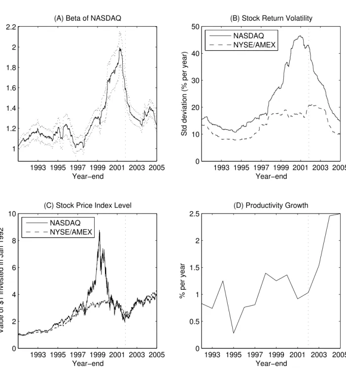
Figure 8 is an empirical counterpart of Figure 7 for the period 1992–2005. For simplicity, we assume that the technology-loaded NASDAQ index represents the new economy and the NYSE/AMEX index is the old economy. We obtain daily index returns from CRSP.
Panel A of Figure 8 plots the market beta of the NASDAQ index, along with its two-standard-error confidence bands. The beta is computed daily as the slope coefficient from the regression of the NASDAQ returns on the NYSE/AMEX returns over the most recent 500 trading days (i.e., about two years). After a slight decrease from about 1.2, NASDAQ’s beta doubles from 1.0 to 2.0 between 1997 and mid-2002, and this increase is highly statistically significant. This empirical pattern is strikingly similar to the model-implied pattern in Panel A of Figure 7, in which the beta also decreases by about 0.2 before rising 2.3-fold by the end of the revolution. According to the model, the time when the beta peaks is the time of the large-scale adoption; hence the evidence on NASDAQ’s beta is consistent with the probability of the Internet’s large-scale adoption reaching one by mid-2002.
Panel B of Figure 8 plots the standard deviations of returns on the NASDAQ and NYSE/AMEX indices, computed daily over the most recent 500 trading days. NASDAQ’s volatility falls from 17% in 1992 to 11% in 1995, before rising to 47% at the beginning of
role as a leader in the new world economy, while redefining what the next generation of digital-based leaders will look like.” (CNN Money, Jan 10, 2000).
2002. NYSE/AMEX’s volatility falls from 13% in 1992 to 8% in 1995, before rising to 21% by the end of 2002. These patterns are similar to the model-implied patterns in Panel B of Figure 7 in several ways: (i) the new economy’s volatility always exceeds the old economy’s volatility; (ii) both volatilities generally rise over time, with a bit of a U-shape pattern; (iii) the new economy’s volatility rises much faster; and (iv) both volatilities peak at about the same time. In the model, both volatilities peak at the time of the adoption; the volatility evidence is thus consistent with the Internet revolution ending sometime in 2002.
Panel C of Figure 8 plots the index levels for NASDAQ and NYSE/AMEX, namely, the value of $1 invested in these indices in January 1992, with dividend reinvestment. The NASDAQ index quadruples between 1996 and March 2000, but then it falls back to the 1996 level by October 2002, after which it rises again. In contrast, NYSE/AMEX exhibits a much smaller rise and fall over the same period. This pattern is similar to the model-implied pattern in Panel C of Figure 7, in which the new economy’s market value also exhibits a “bubble” but the old economy’s rise and fall are much less pronounced.12 According to the
model, the time when both indices stop falling is the time of the large-scale adoption; hence this evidence is consistent with the Internet’s adoption by October 2002.
Panel D of Figure 8 plots a three-year moving average of multifactor productivity growth in the private business sector of the U.S. economy. (This is the most commonly used multi-factor productivity measure, according to the Bureau of Labor Statistics, which is the source of the data.) In year t, we plot the average annual productivity growth in years t−2,t−1, and t. Multifactor productivity growth averaged about 1% per year in the 1990s, but it increased sharply after year 2002: from 1% per year in 2002 to 1.5% in 2003 and 2.5% in 2004 and 2005. A similar pattern is observed for labor productivity.13 The observed
pro-ductivity pattern is similar to the model-implied pattern in Panel D of Figure 7, except that
12
P´astor and Veronesi (2006) show that NASDAQ’s M/B dropped by 5.3 (from 8.5 to 3.2) from the peak to the bottom in 2.7 years. Both the duration and the magnitude of this drop in M/B correspond closely to their counterparts in our model. The corresponding model-implied average pattern in M/B is plotted in Panel D of Figure 5 (in which the revolution lasts 6 years, as it does in Figure 7). This average M/B falls by 4.5 from the peak to the bottom, also in 2.7 years, matching the observed values remarkably closely.
13
In his Remarks Before Leadership South Carolina on August 31, 2006, Ben Bernanke argued that “One of the most important economic developments in the United States in the past decade or so has been a sustained increase in the growth rate of labor productivity... From the early 1970s until about 1995, productivity growth in the U.S. nonfarm business sector averaged about 1.5% per year... Between 1995 and 2000, however, the rate of productivity growth picked up significantly, to about 2.5% per year... Talk of the “new economy” faded with the sharp declines in the stock valuations of high-tech firms at the turn of the millennium. Yet, remarkably, productivity accelerated further in the early part of this decade. From the end of 2000 to the end of 2003, productivity rose at a 3.5% annual rate and it is estimated to have increased at an average annual rate of 2.25% since the end of 2003. These advances were achieved despite adverse developments that included the 2001 recession, the terrorist attacks of September 11, [etc.].”
that figure plots the level of productivity as opposed to its growth rate.14 In the model,
the economy’s productivity begins rising at the time of the adoption; hence the productivity evidence is consistent with a large-scale adoption of the Internet by 2002.
Overall, we find Figure 8 remarkably similar to Figure 7. The patterns of NASDAQ’s beta and NYSE/AMEX’s volatility show that both sectors experienced large increases in systematic risk in 1997–2002, supporting the key prediction of the model. To summarize, the empirical evidence seems consistent with the joint hypothesis that our model holds and that the Internet technology was adopted on a large scale by 2002.
5.2.
American Railroads Before the Civil War
Our paper is motivated by the technological revolutions, listed in the introduction, that were accompanied by apparent bubbles in stock prices. In this section, we conduct an “out-of-sample” analysis of a revolution whose stock prices do not seem to have been analyzed before. We analyze the first major technological revolution that took place in the U.S. since the New York Stock Exchange was organized in 1792 – the introduction of steam-powered railroads (RRs). In the early days of the RR, there was substantial uncertainty about whether the RR technology would be ultimately adopted on a large scale. After examining the historical milestones of American RRs in Section 5.2.1., we argue that the probability of a large-scale adoption rose gradually, and that it approached one in the late 1850s after the RR expansion west of the Mississippi River. We then empirically examine the behavior of the RR stock prices in 1830–1861 in Section 5.2.2. In the context of our model, our evidence is consistent with a large-scale adoption of the RR technology around year 1857.
5.2.1. Brief History
The steam engine, an 18th-century invention, was first used for rail-based transportation in the early 19th century in Britain. The United States followed shortly afterwards. The first RR act in the U.S. was passed in 1815 when the New Jersey legislature awarded a charter to Colonel John Stevens to build a RR between the Delaware and Raritan rivers.15
In 1825, Stevens operated the first locomotive in America – his 16-foot “Steam Waggon” ran around a circular rail track in Hoboken at 12 miles per hour. The construction of the first RR, the Baltimore & Ohio, began in July 1828. The Baltimore & Ohio initially used
14
Our comparison seems reasonable because in the model, average productivity can grow only via techno-logical revolutions, whereas in reality, there are also many non-revolutionary improvements in productivity. Therefore, in the data, it is the growth rate of productivity that sets a technological revolution apart.
15
horses to draw its cars, but it replaced them in 1830 by a steam locomotive, Peter Cooper’s “Tom Thumb.” In 1830, both passenger and freight service commenced on the Baltimore & Ohio. RRs spread quickly. On Christmas Day in 1830, the “Best Friend of Charleston,” the first locomotive built for sale in the U.S., made the first scheduled steam-RR train run in America. Between 1830 and 1840, the RR mileage in the U.S. grew from 23 to 2,808 miles. In 1840, only four of the 26 states had not completed their first mile of track.
The new RR technology competed with the existing modes of transportation such as wagons, stagecoaches, steamboats, and canals. Those were not without problems – wagons were slow and expensive, stagecoaches were uncomfortable, steamboats were dangerous and limited in scope, and canals froze over in winter. However, it was far from obvious in the 1830s and 1840s that the RRs would later come to dominate the transportation industry. For example, waterways were much less expensive than RRs, and wagons were not restricted to rails. While the RR mileage caught up with the canal mileage in the early 1840s, waterways still carried the great bulk of the nation’s freight in the late 1840s. Writes Fogel (1964): “Far from being viewed as essential to economic development, the first RRs were widely regarded as having only limited commercial application. Extreme skeptics argued that RRs were too crude to insure regular service, that the sparks thrown off by belching engines would set fire to buildings and fields, and that speeds of 20 to 30 miles per hour could be “fatal to wagons, road and loading, as well as to human life.” More sober critics questioned the ability of RRs to provide low cost transportation, especially for heavy freight. [Some] placed “a RR between a good turnpike and a canal” in transportation efficiency.”
Nearly all RRs organized as corporations funded by private investors. More than half of the more than $300 million invested in American RRs in 1850 was represented by capital stock, the remainder being in bonds. The freight business was economically more important than passenger traffic, which typically produced around 30% of the total revenue.
While most early RRs were built with local capital to provide local transportation, RR building became more ambitious in the 1850s. This decade “was one of the most dynamic periods in the history of American RRs” (Stover, 1961). RR mileage expanded from 9,021 in 1850 to 30,626 in 1860, and total investment in the industry increased from about $300m to about $1,150m over the same period. This growth was spurred by land grants to RRs by the federal government. The first land-granting act was passed by the Congress in 1850, aiding the Illinois Central and the Mobile & Ohio RRs. The RR growth in the 1850s was also stimulated by the discovery of gold in California and the lure of the trans-Pacific trade. In the 1850s, New York, Philadelphia, and Baltimore all achieved their rail connections with
the west. In 1853, an all-rail route opened from the East to Chicago, and Chicago quickly became the rail capital of the nation. The RR technology also advanced in the 1850s – telegraph was first used to dispatch trains, T-rails became the general rule, and so did the standard track gauge, at least in the North.16 “Instead of merely serving as connectors
between navigable bodies of water as originally conceived, RRs were replacing them as the preferred way of transport” (Klein, 1994).
The dramatic RR growth in the 1850s is also evident in Figure 9, which plots the total rail consumption in the U.S., measured by the number of track-miles of rails laid each year (Fogel, 1964). Rail consumption grew fast in the 1830s, but especially fast during the decade leading up to 1856. After 1856, rail consumption slowed down and even declined in 1861 when the Civil War began, but it accelerated again after the war.
The diffusion of the RR technology made a leap in 1856 when two milestone RRs were completed: the Illinois Central, the longest RR in the world (705 miles), and the Sacramento Valley, the first RR in California. Also in 1856, the first RR bridge across the Mississippi was built near Davenport, Iowa, heralding future westward expansion into the region then known as the “Great American Desert.” This westward expansion was the defining feature of the RR growth in the decades to come. The RRs shaped the economy of the West, creating new national markets and fostering unprecedented economic specialization across the nation.
By the late 1850s, it seemed clear that the RR had become a dominant form of trans-portation. According to Stover (1961), “By 1860 the canal packets and river steamers had lost much of their passenger traffic” to the RR. In 1860, every state save Minnesota and Oregon had RR mileage, and 29 of the 33 states had more than 100 miles of line. Klein (1994) argues that “By 1860... [the RR] had emerged not only as the preferred form of transportation but also as the chief weapon of commercial rivalry.” This evidence suggests that a large-scale adoption of the RR technology took place by the end of the 1850s.
5.2.2. Railroad Stock Prices
To examine the behavior of RR stock prices in the early days of the RR (1830–1861), we use the data compiled by Goetzmann, Ibbotson, and Peng (2001). These data contain monthly individual stock prices for NYSE stocks from 1815 to 1925, as well as annual dividends for a
16
The Northern RRs were using 11 different track gauges in the 1850s, but the standard gauge, 4’8.5”, became by far the most common by 1860, according to Stover (1961). The South was still mostly on the 5’ gauge. Benmelech (2007) exploits the diversity of track gauges in 19th century American railroads to examine the effect of asset liquidation value on capital structure.
subset of stocks from 1825 to 1870. The data are provided at http://icf.som.yale.edu/nyse/. To focus on common stocks, we exclude stocks classified as “preferred” or “scrip” in the database. (Scrips are certificates convertible into shares when fully paid-in.) If such classification is not provided, we examine the stock name and exclude stocks whose name contains an indication of non-common status such as “pref,” “pr.,” “pf,” or “scrip.” Among the 671 stocks in the database, we identify and exclude 85 preferred stocks and 29 scrips.
We identify 284 RR stocks (42.32% of the whole sample) by examining the stock names. The first RRs that appear in our price index (discussed below) in 1831 are Camden & Amboy, Canajoharie & Catskill, Harlem, and Ithaca & Oswego. All RRs that have at least one valid monthly common stock return between 1830 and 1861 are listed in Table 2.
We clean the monthly price file to remove apparent data errors. To proceed in a system-atic fashion, we exclude all prices that imply implausibly large return reversals. Specifically, we exclude prices that more than tripled compared to the most recent available price and then fell to less than a third at the nearest future observation, as well as prices that experi-enced the same reversals in reverse order (first down, then up). We eliminate 34 such prices in our 1830–1861 sample. We also examine all price sequences in which the price increased or decreased at least tenfold without reversal, and eliminate six suspicious price entries between 1830 and 1861. We retain the price entries that imply returns below -90% at the very end of a stock’s price series because these could be stocks heading for bankruptcy. Altogether, we delete 40 of the 15,276 price entries between 1830 and 1861, or 0.26% of the sample.
Before the price coverage in the database improves in 1848, uninterrupted price sequences for RR stocks are rare. In no month before 1848 are there more than five RR stocks with valid monthly returns, and there are months with zero RR returns. An important part of the problem are gaps in the price series, in which one or several missing values are sandwiched between two valid prices for a given stock. To alleviate the data shortage, we fill in such gaps by linear interpolation, but only for gaps that are no more than three months long. This procedure substantially increases the price coverage early in the sample. For example, without interpolating, the RR year-end price-dividend ratio discussed below would have only three valid observations prior to 1847; with interpolation, the number of valid observations increases to eight. Without interpolating, our results would be noisier, with more missing values, but they would lead to the same basic conclusions.