Understanding the Performance of the Java Operating System JX using Visualization Techniques

(1)

Understanding the Performance of the Java Operating System JX

using Visualization Techniques

Michael Golm, Christian Wawersich, Jörg Baumann, Meik Felser, Jürgen Kleinöder

Dept. of Computer Science

University of Erlangen-Nuremberg

{golm, wawersich, bauman, felser, kleinoeder}@informatik.uni-erlangen.de

Abstract

During the development of the Java-based operating

sys-tem JX, we frequently needed tools to assess the

perfor-mance of the microkernel and the Java components. We

instrumented the microkernel and the

bytecode-to-native-code translator to get information about nearly every aspect

of the systems behavior. The gathered data can be visualized

to show CPU time consumption of methods, thread

schedul-ing, object allocation behavior, and object ages.

1 Introduction

In the JX project [4][5] we build a complete operating

sys-tem using the type-safe, object-oriented language Java. One

of the major challenges is achieving a performance that is

competitive to mainstream operating systems, such as

Linux or Solaris. It is in the nature of our microkernel-based

system, that most time is spent executing Java code.

Achiev-ing a good performance therefore requires an optimizAchiev-ing

bytecode-to-nativecode translator and instrumentation/

visualization tools to locate performance problems. In this

paper we concentrate on the second requirement. To

illus-trate the various instrumentation and visualization

tech-niques we use one single application: an NFS server that is

written in Java (as are the RPC/UDP/IP/device driver

lay-ers) and runs on the JX microkernel.

Reed [10] classifies performance instrumentation into

timing, counting, sampling, and tracing. The method timing

system is described in Section 2, Section 3 describes our

sampling system, Section 4 the event tracing. Section 5

describes our tools to assess the memory usage behavior of

the system. The problems that we solved concerning data

collection and transfer are described in Section 6.

2 Method timing

To write faster code, it is necessary for the programmer to

identify the most time-consuming parts of a program. These

hot spots of execution often indicate poor code or

bottle-necks. The hot spots are the parts of the code that benefit

most from optimizations. We instrumented the

bytecode-to-nativecode translator to insert code that measures the

execu-tion times of methods. Method timing creates an overhead

particularly at small methods. To get more exact results, we

use several error correction techniques.

Hardware supported measuring. Method timing uses the

time stamp counter register (TSC) of the Pentium processor

family. The TSC contains the elapsed clock ticks since

sys-tem boot. To measure the time consumed by a method, we

save the TSC in the prolog of the method and subtract the

TSC in the epilog of the method. The result is totalized for

each invocation pair consisting of caller and callee method.

The sum is saved together with the number of invocations

and the caller and callee address in a data structure per

thread. Collecting the data separately per thread avoids

locking overhead and allows to analyze the behavior of a

dedicated thread.

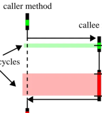
Error correction. Figure 1 shows the flowchart of a single

method invocation. The measurement of the callee method

caused an overhead (extra clock cycles) that falsifies the

result.

The extra cycles are wrongly accounted to the caller

method. To avoid this measurement error, it is necessary to

identify the consumed extra clock cycles. The amount of

extra cycles in the prolog is almost constant and it is

possi-ble to determine a fix value. The more significant and

caller method

callee method

extra cycles

prolog

epilog

method body

(2)

changing number of extra cycles in the epilog is measured

by reading the time stamp count a third time and computing

the number of extra cycles.

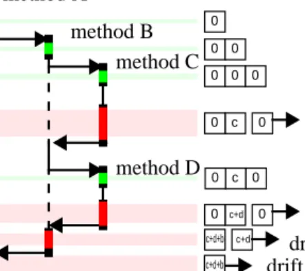
For error correction of a deeper nested method we have

to accumulate the quantified drift and propagate the drift to

the callers. A stack is used for this task. Figure 2 illustrates

the functionality of the stack. On every method invocation

the stack is growing by a new initialized counter. The drift

for a particular method (the small letters in Figure 2) is

always accumulated on the topmost counter. In the epilog of

a method the topmost counter is popped from the stack and

subtracted from the measured clock cycles of the method.

Then the drift is added to the drift of the caller method.

In this way the error made by the measurement is

suffi-ciently compensated for a single thread. This is sufficient to

find the most–time-consuming parts of a program or to

examine the execution path. But it is not sufficient to

deter-mine the exact execution time for a single method or to

determine the variation, because the execution of extra code

during the measurement has noticeable impact on the

mem-ory bandwidth, the caches, the buffers, and the branch

pre-diction of the processor. To measure the exact execution

time of a single method the translator can be configured to

insert the measurement code only into the prolog and epilog

of that method.

Support of multithreading. The JX system, as a Java

run-time environment, usually has more than one thread of

exe-cution. While profiling is active the system scheduler has to

inform the profiler about the suspension of a thread. In this

case the number of clock cycles during the suspension

period is computed. If the thread is suspended outside the

measurement routine the computed value is added to the

current drift counter.

Analyzing the results. To get a better overview of the

exe-cutions paths we produce diagrams that show the execution

times.

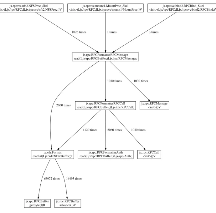
A call graph display (Figure 3) is produced by using the

dot program [1]. After having produced several call graphs

we concluded that this visualization is not well-suited to

give a good picture of the consumed time. This was the

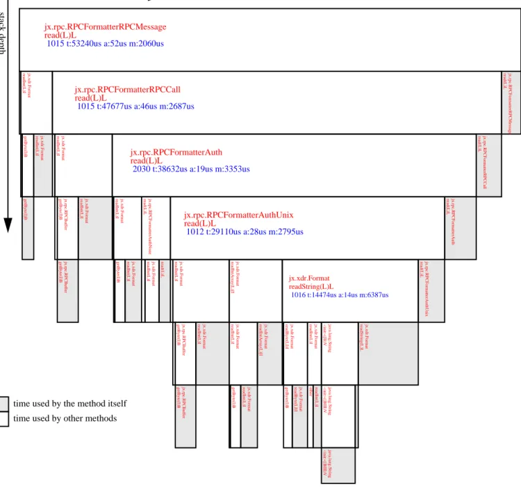
rea-son to develop another visualization (Figure 4) that shows a

box for each method, where the size of the box is

propor-tional to the time consumed by this method.

3 Sampling

Similar to method timing, sampling is used to find hotspots

in the system, but with an considerably lower measurement

overhead. While timing measures the exact execution times

of methods, sampling can only produce a statistical view of

the system. The timer interrupt service routine (ISR) logs

the instruction pointer of the interrupted instruction. The

distribution of the instruction pointers indicates where the

program spends most of its time.

4 Event tracing

User-generated events. JX allows Java components to log

component-specific events. The Java code can register an

event name at the microkernel and gets an event number.

This number is used for subsequent logging. Time and event

number are stored in main memory. The overhead of

log-ging an event is 45 CPU clock cycles.

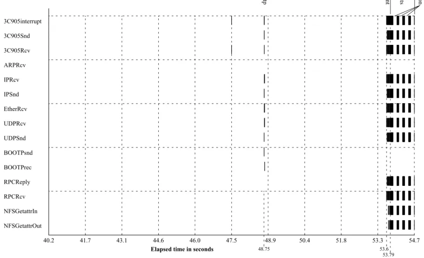
Figure 5 shows the event trace that is produced when the

system boots and acts as an NFS server. The system first

sends a bootp request and receives a reply packet (at about

48.75 sec.). Then the client mounts the NFS file system, and

starts to read the same file in an endless loop. This creates

RPC and NFS traffic starting at about 53.6 sec. 0.2 sec. later

there starts a dense block of events. These are the getattr

requests that are sent by the client during the execution of

the benchmark program. The block of events is interrupted

three times by the garbage collector, that in the current

ver-sion of JX disables all interrupts. This will be changed when

the protocol between GC and intra-domain scheduler is

fin-ished.

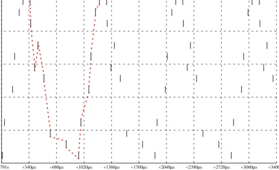
To improve the NFS request rate, we have to look at the

events in more detail, so we zoom into the 3.4 millisecond

interval starting at about 53.791 sec. (Figure 6). There is an

obvious pattern of consecutive events (dotted line) that

starts and ends with a 3C905interrupt event. A complete

cycle needs about 905

µsec. Figure 7 displays the times

between successive events.

Method enter/exit events. For debugging purposes it is

often interesting to know which methods are executed in

which order. Our translator can be configured to insert a

prologue that logs TSC and method pointer. The same

event-recording facilities as with user-generated events are

used. Therefore the diagram looks similar.

0

0 c

0

0 c

0

c+d

0

c+d c+d+b c+d+b

method A

method B

method C

method D

drift of C

drift of D

drift of B

drift of A

(3)

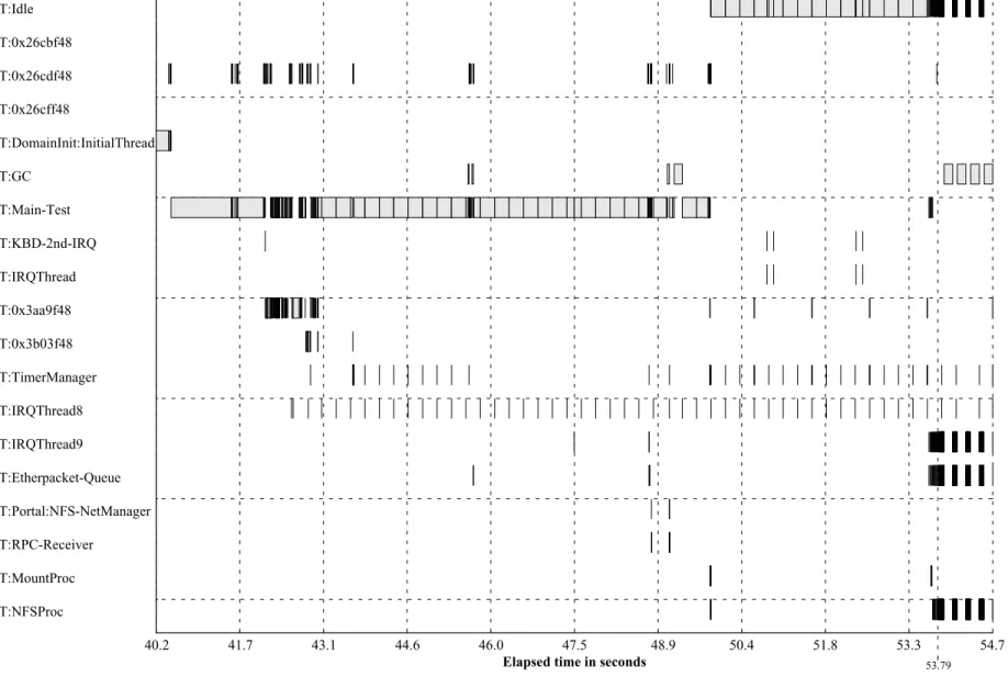
Scheduling events. To visualize the scheduling behavior of

the system we use a thread activity diagram. The kernel is

instrumented to collect events during thread switching. The

TSC and target thread ID are logged.

Figure 8 shows the thread activity during boot and the

NFS test. The y-axis shows either the thread name or the

thread ID for unnamed threads. Some background

informa-tion is necessary to understand this diagram. “Idle” is the

thread that runs when no other thread is runnable. The

“Main-Test” thread is the thread that starts the NFS server.

“IRQThread8” is the first-level interrupt handler for the

RTC interrupt. It runs periodically and fires timers by

unblocking other threads. As “IRQThread8” is a first-level

handler it runs with interrupts disabled and must complete

in a bounded time. Time-consuming tasks are delegated to

the “TimerManager” thread. At about 53.79 sec. the system

starts to receive getattr NFS requests and the thread

switches start to occur more frequently. “IRQThread9” is

the first level interrupt handler for the NIC (network

inter-face card) interrupt. It acknowledges the received packet

with the NIC, places it in a queue, and unblocks the

“Ether-packet-Queue” thread that processes that queue.

5 Memory

Java uses an automatic memory management called garbage

collection. The programmer creates objects but never

destroys them. This is very convenient for the programmer.

But during performance debugging or in order to find

mem-ory leaks the programmer wants to know exactly when

objects are allocated and destroyed.

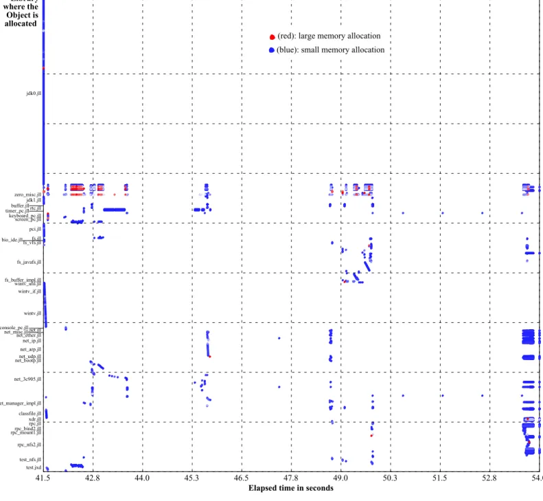
Object creation: time, size and code position. Figure

9 shows at which times and in which libraries, classes, and

methods objects are allocated. The object size is

color-coded: blue means a small, red a large allocation.

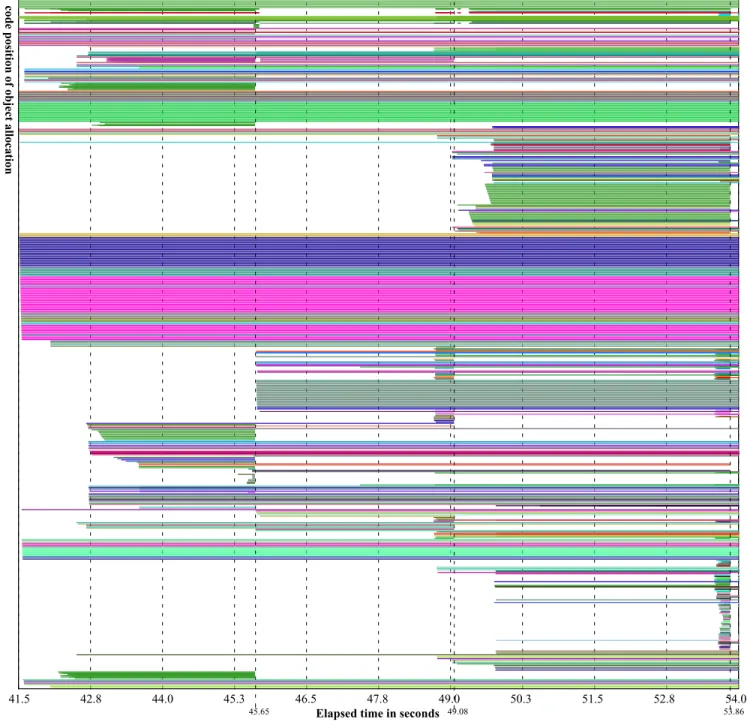
Object creation and destruction. Figure 10 shows the

lifetime of objects. The y-axis shows the instruction pointer,

representing the position of the object allocation (equally

distributed). The color relates to the object type (class). At

one allocation point always the same type of object is

cre-ated. At about 45.65 sec., 49.08 sec. and 53.86 sec. we can

recognize a garbage collector run destroying many objects.

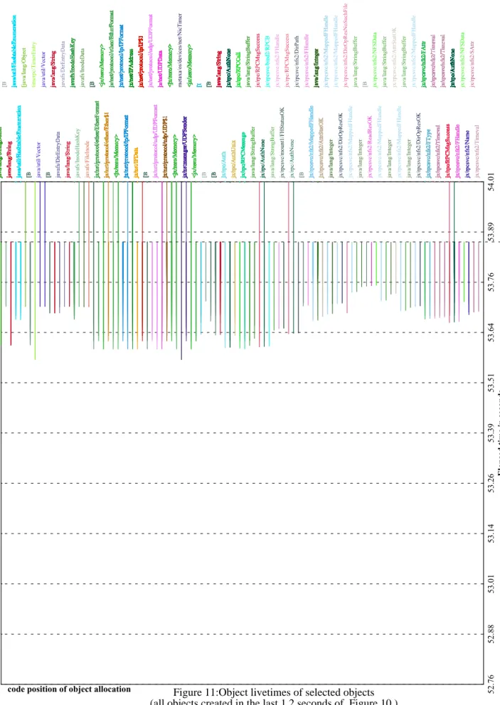
Figure 11 presents a closer look at the objects that are

cre-ated in the last tenth of the diagram in Figure 10.

Object aging. We developed several visualizations to

cap-ture whether objects are long- or short-living and what kind

of objects are more likely to have a long or short lifetime.

Figure 12 shows the age of objects and where they are

allo-cated. The time is measured in allocated memory, that

means an object grows older when memory is allocated.The

number of instances of a class with a certain age is encoded

in the size of the dot. The red line is the average number of

instances with the specific age.

Cache behavior. Figure 13displays the values of the

Pen-tium III performance counters and the thread activity

dia-gram of Figure 8 in the background. During this test the

per-formance counters are configured to measure the number of

lines evicted from the L2 cache and the number of L2

requests. Together with the thread activity diagram the

per-formance counter diagram tells us that there is lot of cache

activity (many accesses and misses) during the boot phase.

Then the code has only few accesses to the L2 cache. Most

requests seem to be satisfied by L1. There is a three seconds

interval where the line is absolutely horizontal. During this

period the system is idle after the initialization of the NIC.

The following steep rise of the curve is created by the GC,

which has poorer locality than the rest of the system.

6 Data collection and transfer

JX is a microkernel with minimal built-in device support.

From a software engineering perspective this architecture is

superior to monolithic OS architectures. Due to the lack of

built-in device drivers and file systems, a microkernel

archi-tecture makes it very difficult to transfer the collected data

from the target system to the outside world. Only the serial

device is supported by the JX microkernel. It is used for

debugging and data transfer.

Especially the GC-aging instrumentation may generate

up to hundreds of megabytes of data. It is very unpractical

to transfer this data in a textual representation via the serial

line. Therefore we transfer it in compressed binary format

using the minilzo [8] compression library.

7 Related work

JVMPI. The Java Virtual Machine Profiler Interface

(JVMPI) is an event-based interface between a JVM and a

profiler agent. Whenever something interesting happens

inside the VM (method is entered or exited, object is

allo-cated, moved, or freed, etc.) the profiler agent is notified.

The profiler agent is also allowed to instrument a class file

after it has been loaded. Because the JVMPI is intended as

a standard interface between different JVMs and profilers

the profiler and JIT are not as tightly integrated as in JX. The

ability of the bytecode-to-native-code translator to insert

special profiling code allows to reduce the measurement

error and to collect trace data with very low overhead.

Fur-thermore, JX allows to collect hardware-specific data using

the CPU’s performance counters, which is essential for the

optimization of the translator.

Hyperprof. Hyperprof uses the data generated by an

unmodified JVM when the “-prof” switch is used. It shows

caller-callee relations and method timing as hyperbolic tree.

While our visualization is not that spectacular it

(4)

neverthe-less makes the same information visually available (method

timing diagram).

Jinsight. IBM’s Jinsight uses a modified JVM to get more

detailed trace information. It is able to display thread

activ-ity, object usage and creation, and garbage collection. It also

provides special features to help diagnosing memory leaks.

As indicated in the previous sections, we can perform

simi-lar diagnostics.

JaViz. JaViz is another performance visualization tool that

collects trace data using a modified JVM. The main focus of

this tool is the analysis of client/server applications. After

collecting and merging the data a call graph can be

dis-played including client/server interaction. While our

profil-ing tools are not designed to merge data collected on

differ-ent computers, it is possible to trace the interaction between

different applications.

Commercial tools. There are also some commercial tools

to profile applications. For example Rational Quantify [9]

counts individual machine cycles by inserting counting

instructions into the object code for every functional block

of code.

JProbe (Sitraka Software) [11], OptimizeIt (Intuitive

Systems Inc.) are similar tools. They all provide a call graph

display, memory usage diagrams etc.

8 Conclusion and future work

A comprehensive analyses of a Java-based OS needs several

instrumentation and visualization techniques.

Instrumenta-tion techniques range from very invasive method timing and

object aging analysis to low overhead application generated

events. The captured data is currently visualized by

gener-ating a FrameMaker MIF file. The MIF backend should be

easily replaceable by other backends, e.g., for X11, which

allow an interactive selection of the interesting data by

spec-ifying time ranges, event types, or object types.

9 References

[1] AT&T Labs-Research: dot-Tool, part of Graphviz - open

source graph drawing software.

http://www.research.att.com/sw/tools/graphviz/

[2] V.Bulatov: HyperProf(v.1.3) - Java profile browser.

http://www.physics.orst.edu/~bulatov/HyperProf/

[3] J. Guitart, J. Torres, E. Ayguadé and J. Labarta. Java

Instru-mentation Suite: Accurate Analysis of Java Threaded

Appli-cations. 2nd Workshop on Java for High Performance

Com-puting, Santa Fe, New Mexico (USA), pp. 15-25. May 2000.

[4] M. Golm, J. Kleinöder: The JX Project.

http://www4.informatik.uni-erlangen.de/Projects/JX/

[5] M. Golm, J. Kleinöder, F. Bellosa: Beyond Address Spaces

- Flexibility, Performance, Protection, and Resource

Man-agement in the Type-Safe JX Operating System. Proc. of

HotOS 2001, May 20-23, 2001, Schloß Elmau, Germany.

[6] IBM: Jinsight - A tool for visualizing and analyzing the

exe-cution of Java programs.

http://www.alphaworks.ibm.com/formula/jinsight

[7] I. H. Kazi, D. P. Jose, B. Ben-Hamida, C. J. Hescott, C.

Kwok, J. A. Konstan, D. J. Lilja, and P.-C. Yew: JaViz: A

client/server Java profiling tool, IBM Systems Journal, 39

(1) , 2000 (http://www.research.ibm.com/journal/sj/391/

kazi.html)

[8] M. Oberhumer: LZO - a portable lossless data compression

library.

http://wildsau.idv.uni-linz.ac.at/mfx/lzo.html

[9] Rational: Rational Quantify for Unix.

http://www.rational.com/products/quantify_unix/index.jsp

[10] D. A. Reed: Performance Instrumentation Techniques for

Parallel Systems. L. Donatiello and R. Nelson (eds), Models

and Techniques for Performance Evaluation of Computer

and Communications Systems, Springer-Verlag, LNCS,

1993, pp. 463-490.

[11] Sitraka: JProbe - Java profiling and testing tools.

http://www.sitraka.com/software/jprobe/

(5)

jx.rpc.RPCFormatterRPCMessage

read(Ljx/rpc/RPCBuffer;)Ljx/rpc/RPCMessage;

jx.rpc.RPCFormatterRPCCall

read(Ljx/rpc/RPCBuffer;)Ljx/rpc/RPCCall;

1030 times

jx.xdr.Format

readInt(Ljx/xdr/XDRBuffer;)I

2060 times

jx.rpc.RPCMessage

<init>()V

1030 times

jx.rpcsvc.nfs2.NFSProc_Skel

<init>(Ljx/rpc/RPC;ILjx/rpcsvc/nfs2/NFSProc;)V

1026 times

jx.rpcsvc.mount1.MountProc_Skel

<init>(Ljx/rpc/RPC;ILjx/rpcsvc/mount1/MountProc;)V

1 times

jx.rpcsvc.bind2.RPCBind_Skel

<init>(Ljx/rpc/RPC;ILjx/rpcsvc/bind2/RPCBind;)V

3 times

jx.rpc.RPCCall

<init>()V

1030 times

4120 times

jx.rpc.RPCFormatterAuth

read(Ljx/rpc/RPCBuffer;)Ljx/rpc/Auth;

2060 times

jx.rpc.RPCBuffer

getByte(I)B

65972 times

jx.rpc.RPCBuffer

advance(I)V

16493 times

(6)

Figure 4:

Method timing

jx.rpc.RPCFormatterRPCMessage

read(L)L

1015 t:53240us a:52us m:2060us

jx.rpc.RPCFormatterRPCMessage

read(L)L

jx.rpc.RPCFormatterRPCCall

read(L)L

1015 t:47677us a:46us m:2687us

jx.xdr.Format readInt(L)I jx.rpc.RPCFormatterRPCCall read(L)L

jx.rpc.RPCFormatterAuth

read(L)L

2030 t:38632us a:19us m:3353us

jx.xdr.Format readInt(L)I jx.rpc.RPCFormatterAuth read(L)L

jx.rpc.RPCFormatterAuthUnix

read(L)L

1012 t:29110us a:28us m:2795us

jx.rpc.RPCFormatterAuthNone read(L)L jx.xdr.Format readInt(L)I jx.rpc.RPCFormatterAuthUnix read(L)L

jx.xdr.Format

readString(L)L

1016 t:14474us a:14us m:6387us

jx.xdr.Format readIntArray(L)[I jx.xdr.Format readInt(L)I jx.xdr.Format readString(L)L java.lang.String <init>([B)V jx.xdr.Format readInt(L)I jx.xdr.Format readByte(LI)I java.lang.String <init>([BIII)V java.lang.String <init>([BIII)V readInt(L)I other jx.xdr.Format readByte(LI)I getByte(I)B jx.xdr.Format readIntArray(L)[I jx.xdr.Format readInt(L)I jx.xdr.Format readInt(L)I getByte(I)B jx.xdr.Format readInt(L)I jx.rpc.RPCBuffer getByte(I)B jx.rpc.RPCBuffer getByte(I)B read(L)L jx.xdr.Format readInt(L)I jx.xdr.Format readInt(L)I getByte(I)B jx.xdr.Format readInt(L)I jx.rpc.RPCBuffer getByte(I)B jx.rpc.RPCBuffer getByte(I)B jx.xdr.Format readInt(L)I getByte(I)B getByte(I)B

stack depth

time consumed (proportional)

time used by the method itself

time used by other methods

(7)

Figure 5:

Application-generated events

mount

getattr requests

garbage collection

40.2

41.7

43.1

44.6

46.0

47.5

48.9

50.4

51.8

53.3

54.7 Events

3C905interrupt

3C905Snd

3C905Rcv

ARPRcv

IPRcv

IPSnd

EtherRcv

UDPRcv

UDPSnd

BOOTPsnd

BOOTPrec

RPCReply

RPCRcv

NFSGetattrIn

NFSGetattrOut

53.6

53.79

48.75 bootp

(8)

Figure 6:

Event trace

53.791s

+340

µ

s

+680

µ

s

+1020

µ

s

+1360

µ

s

+1700

µ

s

+2040

µ

s

+2380

µ

s

+2720

µ

s

+3060

µ

s

+3400

µ

s

Elapsed time (starting at 53.79 sec.)

3C905interrupt

3C905Snd

3C905Rcv

ARPRcv

IPRcv

IPSnd

EtherRcv

UDPRcv

UDPSnd

BOOTPsnd

BOOTPrec

RPCReply

RPCRcv

NFSGetattrIn

NFSGetattrOut

Figure 7:

Time between events

3C905interrupt

6 3C905Rcv

54 EtherRcv

43 IPRcv

83 UDPRcv

82 RPCRcv

210 NFSGetattrIn

168 NFSGetattrOut

29 RPCReply

99 UDPSnd

26 IPSnd

56 3C905Snd

49 3C905interrupt

(9)

Figure 8:

Thread activity diagram

Elapsed time in seconds

T:0x3aa9f48

T:Etherpacket-Queue

T:0x3b03f48

T:GC

T:DomainInit:InitialThread

T:0x26cdf48

T:NFSProc

T:Idle

T:Portal:NFS-NetManager

T:TimerManager

T:Main-Test

T:KBD-2nd-IRQ

T:IRQThread9

T:0x26cff48

T:RPC-Receiver

T:0x26cbf48

T:MountProc

T:IRQThread8

T:IRQThread

40.2

41.7

43.1

44.6

46.0

47.5

48.9

50.4

51.8

53.3

54.7

53.79

(10)

Figure 9:

Object allocations over time

41.5

42.8

44.0

45.3

46.5

47.8

49.0

50.3

51.5

52.8

54.0 Elapsed time in seconds

test.jxd test_nfs.jll rpc_nfs2.jll rpc_mount1.jllrpc_bind2.jll rpc.jll xdr.jll classfile.jll net_manager_impl.jll net_3c905.jll net_bootp.jllnet_udp.jll net_arp.jll net_ip.jll net_ether.jll net_misc.jll net.jll console_pc.jll wintv.jll wintv_if.jll wintv_util.jll fs_buffer_impl.jll fs_javafs.jll fs_vfs.jll bio_ide.jll fs.jll pci.jll screen_pc.jll keyboard_pc.jll timer_pc.jllrtc.jll buffer.jll jdk1.jll zero_misc.jll jdk0.jll