Abstract—The paper presents a one-dimensional transient mathematical model of compressible thermal multi-component gas mixture flows in pipes. The set of the mass, momentum and enthalpy conservation equations for gas phase is solved. Thermo-physical properties of multi-component gas mixture are calculated by solving the Equation of State (EOS) model. The Soave-Redlich-Kwong (SRK-EOS) model is chosen. Gas mixture viscosity is calculated on the basis of the Lee-Gonzales-Eakin (LGE) correlation. Numerical analysis on rapid decompression in conventional dry gases is performed by using the proposed mathematical model. The model is validated on measured values of the decompression wave speed in dry natural gas mixtures. All predictions show excellent agreement with the experimental data at high and low pressure. The presented model predicts the decompression in dry natural gas mixtures much better than GASDECOM and OLGA codes, which are the most frequently-used codes in oil and gas pipeline transport service.
Keywords—Mathematical model, Rapid Gas Decompression I. INTRODUCTION
EW technologies on natural gas production require more intensive gas transmission from one place to another one. A rupture of the pipeline happens and brings numerous problems for oil and gas engineers. The fracture propagation control in gas transport pipeline service is usually performed by using the Battelle two-curve method, which was developed by the Battelle Columbus Laboratories in order to determine of the fracture arrest toughness [1,2]. The fracture propagation speed in the pipeline wall and the decompression wave speed in gas mixtures are required to be employed in the Battelle analysis. The fracture propagation is arrested when the decompression wave speed in gas mixtures is quicker than the fracture propagation velocity in the pipeline wall. Therefore, the information on the decompression wave speed in different natural gas mixtures is very important for the fracture propagation control and pipeline design. The process of the decompression in natural gases is very quick in time. The liquefied fraction is appeared in the shock tube when the temperature and pressure are low enough. The friction due to the liquid appearance significantly changes the decompression speed in natural gases. A transient mathematical model of single- or multiphase flows of multi-component fluid mixtures in a shock tube is highly desirable in this case.
Dr. Evgeniy Burlutskiy was with PETROSOFT-DC, Singapore. He is now with the A*STAR Institute of High Performance Computing (IHPC), 1 Fusionopolis Way, 138632, Singapore (phone: +65 6419 1386; e-mail: [email protected] and [email protected]).
A local distribution of basic flow parameters, which are obtained by using the mathematical modeling, may significantly help in the pipeline design and flow assurance.
The information on the mathematical modeling and experimental study of the decompression in natural gas mixtures is limited in the open source literature. Numerous experimental measurements of the decompression wave speed in rich and dry natural gas mixtures are conducted by TCPL (Trans Canada Pipe Lines) with a high order of accuracy last time [3-7]. The influence of the shock tube inner diameter, gas mixture composition, pressure, and temperature is carefully examined experimentally. Pressure values are varied in those studies in the range between 10 MPa and 37 MPa [3,6]. The temperature is varied from normal values to low [3,5,7]. Most of the measurements are made by using the small-diameter shock tube, where the friction force influences on the flow behavior much stronger compared to large-diameter pipes.
The analytical GASDECOM [1] program is frequently used software in gas transport industry. The decompression wave speed values are successfully calculated by using GASDECOM [3,5]. The program predicts those values with a reasonably good level of accuracy. However, the friction force is not accounted for in the analysis here. The comparison between measured data and GASDECOM’s calculations is usually poor and the values are over-predicted, if the decompression wave speed is determined from the pressure transducers locations, which are mounted far away from the rupture end of the pipe, and where the friction influences on the flow behavior significantly. The over-prediction of the decompression wave speed values is much stronger, if the liquefied fraction is appeared in the shock tube.
The commercial 1D OLGA code [8], which is developed by SPT-group, is the most well-known and frequently used software in the field of oil and gas flow assurance. Numerical simulations of the rapid gas decompression process in rich and dry gas mixtures are performed [5] by using OLGA code as well. All predictions, which are made by using OLGA [5], show a significant over-prediction of pressure time history values and a poor comparison with the experimental data.
The paper presents a one-dimensional transient mathematical model of compressible thermal multi-component gas mixture flow in pipes. Numerical analysis of the decompression in dry natural gases is made on the basis of the proposed mathematical model. The model is successfully validated on the experimental data [5] and it shows a very
Evgeniy Burlutskiy
Numerical Analysis on Rapid Decompression in
Conventional Dry Gases using
One-Dimensional Mathematical Modeling
N
good agreement with the measurements. Predictions, which are made by using the proposed model, are compared in the paper with simulations, which are performed by using the OLGA code and the analytical GASDECOM. Those calculated values (i.e. OLGA and GASDECOM) are taken from [5].
II.ONE-DIMENSIONAL MATHEMATICAL MODEL OF TRANSIENT SINGLE-PHASE FLOW
The set of the mass, momentum and enthalpy conservation equations for the gas phase is solved in the mathematical model. This set of equations for the single phase gas mixture in general form is written as [9]:
0 = ∂ ∂ + ∂ ∂ z U t G G G G Gρ α ρ α (1) Wall G G G G G G G G R z P z U t U − − ∂ ∂ − = ∂ ∂ + ∂ ∂α ρ α ρ 2 α (2) ∂ ∂ + ∂ ∂ = ∂ ∂ + ∂ ∂ z P U t P z h U t h G G G G G G G G Gρ α ρ α α (3)
Here, αG is the volume fraction of the gas mixture; ρG is the density of the gas mixture; U is the velocity of the gas G
mixture; P is the total pressure; RG−Wall is the friction term, h G is the enthalpy of the fluid, t is the time, z is the axial co-ordinate. The friction term is written as [10]:
> = < = = − = − − − − − − − 1600 Re , Re / 316 . 0 1600 Re , Re / 64 , 8 U , S R G 25 . 0 G Wall G G G Wall G 2 G G Wall G Wall G Wall G Wall G ξ ξ ρ ξ τ τ Π (4) G pipe G G G U D / Re =ρ µ (5)
Here, Π is the perimeter of the pipe; S is the cross-sectional area of the pipe; τG−Wall is the friction term (i.e. Gas-Wall interaction); ξG−Wall is the friction coefficient; Dpipe is the diameter of the pipe; µG is the viscosity of the fluid.
III. THERMO-PHYSICAL PROPERTIES OF GAS MIXTURE Thermo-physical fluid properties are modeled by solving of the Equation of State (EOS) in the form of the Soave-Redlich-Kwong model [11]. The set of equations and correlations (SRK-EOS) may be written as [11]:
(
) (
VV b)
a b V T R P + − − = (6)(
)
∑
∑∑
= = = = − = N 1 i i i N 1 i N 1 j ij j i j iz aa 1 k ,b zb z a (7) i C i C i 2 i C i i C 2 i C 2 i P RT 08664 . 0 b , T T 1 m 1 P T R 42748 . 0 a = − + = (8) 2 i i i 0.48 1.574 0.176 m = + ω − ω (9)Here, V is the volume of the gas mixture; N is the number of components in the gas mixture; T is the temperature of the gas mixture; R is the universal gas constant; ωi is the acentric factor of the component i; PCi,TCi are critical values of the pressure and temperature, correspondently; z is the mole i
fraction of the component i. The compressibility factor (Z) of the gas mixture is calculated from the following equation [11]:
(
A B B)
Z AB 0 Z Z3− 2+ − − 2 − = (10) RT P b B , T R P a A= 2 2 = (11) TZ M R P=ρ (12)Here, M is the molar mass of a substance. The viscosity of gas mixture is calculated by using of the Lee-Gonzales-Eakin (LGE) correlation [12]. The algorithm of solving of the set of One- Dimensional transient governing equations of the fluid mixture flow in a pipe is based on the Tri-Diagonal Matrix Algorithm (TDMA), also known as the Thomas algorithm [13]. It is a simplified form of Gaussian elimination that can be used to solve tri-diagonal systems of equations. The set of unsteady governing equations is transformed into the standard form of the discrete analog of the tri-diagonal system [13] by using the fully implicit numerical scheme. In this case the equation is reduced to the steady state discretization equation if the time step goes to infinity.
IV. GAS DECOMPRESSION PROGRAM
A 1D transient mathematical model of compressible thermal multi-component gas mixture flow in pipes was developed under the research project “Multi-component Gas mixture flows in pipelines and wells” in PETROSOFT-DC. This mathematical model was implemented into the FORTRAN computer code and was named the “Gas Decompression Program” (GDP code). More information is available on www.petrosoft-dc.com.
V.NUMERICAL ANALYSIS ON RAPID DECOMPRESSION IN DRY NATURAL GAS MIXTURES
The presented mathematical model was validated [14] on the experimental data on rapid decompression in base natural gas mixtures [3]. The validation of the proposed model on dry gas mixture experimental data of the same authors [5] is presented in this paper. The decompression wave speed
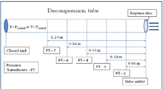
at TCPL Gas Dynamic Test Facility in Didsbury, Alberta, Canada [5] using the same test facility. The main test section of the facility is the shock tube, which has a total length of 172 m. The inner pipe diameter is 49.325 mm. The internal surface of the tube has a roughness, which is better than 1 micron. A rupture disc is placed at one end of the pipe, which is upon rupturing. A decompression wave propagates up into the pressurized test section. High frequency responses Pressure Transducers (PT) are mounted into the tube part, which is most close to the rupture end of the shock tube, in order to capture the time history of the expansion fan [5]. Four pressure-time tracers (PT-2, PT-3, PT-4 and PT-6) were used in order to determinate the decompression wave speed values in those experiments. Distances between pressure transducers PT-2, PT-3, PT-4, PT-6, PT-7 and the rupture disc are 0.06, 0.24, 0.44, 0.84, 1.24 meters, correspondently. Fig. 1 shows the schematic of the experimental decompression tube.
Fig. 1 Schematic of the experimental decompression tube The computational decompression pipe, which has a length of 6 meters long, is simulated by using the proposed model. The set of governing equations is solved on the mesh having 800 grid nodes. The inner pipe diameter is 49.325 mm. One end of the shock tube is selected to be the closed end. The rupture disc condition is modeled in the other end of the pipe. The following initial pressure, temperature and gas compositions (table 1), which are identical to the experimental [5], are chosen to be simulated here:
TABLEI
GAS COMPOSITION (MOLE %),INITIAL PRESSURE (MPA) AND TEMPERATURE (K) Case 1 Case 2 initial P 10.58 20.55 initial T 247.4 248.2 N2 0.569 0.565 CO2 0.781 0.769 C1 95.474 94.986 C2 2.936 3.423 C3 0.190 0.205 i-C4 0.016 0.016 n-C4 0.025 0.026 i-C5 0.004 0.004 n-C5 0.003 0.003 C6+ 0.001 0.002
Two cases (table 1) are simulated using the proposed mathematical model. Predictions are started with the initial pressure of 10.58 MPa and temperature of 247.4 K in each computational cell of the pipe for the case 1. New values of the velocity, temperature, density and pressure are calculated after each time step. The upper limit of the time step is selected from the point of view of the numerical stability of calculations. The decompression is very quick process and basic parameters of gas mixture are changed very rapidly. Therefore, the time step have to be small enough in order to simulate continues change of pressure and temperature values in time at every computational cell. The time step is equal to
5 10
2⋅ − sec in those cases.
The comparison between measured and predicted pressure time history values at PT-2 (fig. 2(a)) and PT-4 and PT-7 (fig. 2(b)) locations are shown in fig. 2. The case 1 (table 1) is simulated first. Experimental points are shown as symbols in all figures here. Continues lines represent calculated values. Numerical predictions of the decompression process in dry gas mixtures in the conditions of the considered case (table 1, case 1) were made by using the commercial 1D OLGA code [5] as well. Those numerical values are taken from [5] and are compared with calculations, which are performed by using the proposed model (fig. 2).
12 13 14 15 16 17 18 19 20 3 4 5 6 7 8 9 10 11 Measured (PT-2) GDP code (PT-2) OLGA code (PT-2) P re ss u re [ M P a] Time [msec] a) 14 16 18 20 22 24 26 4 5 6 7 8 9 10 11 12 Exp (PT-4) GDP (PT-4) OLGA (PT-4) Exp (PT-7) GDP (PT-7) OLGA (PT-7) P re ss u re [ M P a] Time [msec] b)
Fig. 2 Pressure time history at PT-2 (a) and PT-4&PT-7 (b), case 1
Calculations, which are made by using GDP code, are in good agreement with the experimental data. Predicted pressure time history values is decreased under rupturing until the level, which is measured experimentally (i.e. 3.6 MPa at PT-2 and 4.5 MPa at PT-4 locations, fig. 2). The calculated decrease rate (i.e. the slope of the time-pressure curve) is well correlated with the experimental points, too. The pressure time history values, which are calculated by using the OLGA code, show a significant over-prediction (fig. 2). Fig. 2(b) shows that the pressure decrease rate of OLGA’s predictions is much slower compared to the experimental data as well. In general, the OLGA code shows a poor agreement with the measurements. 10 20 30 40 50 60 70 80 -80 -70 -60 -50 -40 -30 -20 Measured (PT-2) GDP code (PT-2) Measured (PT-3) GDP code (PT-3) T em p er at u re [ o C ] Time [msec]
Fig. 3 Temperature time history values at PT-2 and PT-3, case 1
-120 -100 -80 -60 -40 -20 0 5 10 15 20 Phase Envelope case 1 at PT-2 case 2 at PT-2 P re ss u re [ M P a] Temperature [oC]
Fig. 4 Pressure-temperature envelope
The temperature time history is shown in fig. 3. Basing on the fact that the confidence in measured temperature values is low due to late response of the temperature probes on the quick temperature change [5], predicted values are scaled. The collection of time values (i.e. time step) is multiplied on the selected number in order to change the rate of decrease, only. Predicted temperature values are not scaled. Fig. 3 shows the calculations, which are made by using the GDP code. The proposed model reaches measured temperature minimum
values are decreased from the initial temperature level (-25.6oC) to the lowest one (-73oC) within the time of 5-10 msec. Numerical analysis shows, that the non-scaled predicted values of the temperature have much stronger rate of decrease and are decreased from the initial level to the lowest values within the time of 0.5-1 msec at the near rupture end of the pipe.
The pressure-temperature envelope is shown in fig. 4. The liquid fraction is appeared in dry gas mixture for the case 1 when the pressure goes less than 5 MPa and the temperature is lower than -65 Co . The pressure values are increasing after first rapid decrease (fig. 2(a) PT-2 for the time from 15 to 20 ms; and fig. 2(b) PT-4 for the time from 20 to 26 ms) due to the liquid appearance at those locations of the shock tube. Predictions, which are made by using GDP code, do not well correlated with the experimental data in this range because the liquid appearance in the shock tube is not taken into account by the proposed model. An additional friction is produced due to the liquid in the pipe.
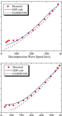
0 100 200 300 400 0.4 0.6 0.8 1.0 Measured GDP code GASDECOM P re ss u re r at io [ -]
Decompression Wave Speed [m/s]
a) 0 100 200 300 400 500 600 0.2 0.4 0.6 0.8 1.0 Measured GDP code GASDECOM P re ss u re r at io [ -]
Decompression Wave Speed [m/s]
b) Fig. 5 Decompression wave speed as a function of pressure ratio,
case 1 (a) and case 2 (b)
Another simulation of the decompression in dry natural gas in the conditions of case 2 (table 1) is performed, too. Fig. 5 shows measured and predicted values of the decompression wave speed, which are determined from PT-2, PT-3, PT-4 and PT-6 pressure transducer locations. Pressure values are
lines represent calculations, which are made using GDP code. Broken curves represent GASDECOM numerical results. Predicted values of the decompression wave speed in dry gases, which are performed by using the analytical GASDECOM [1], are taken from [5]. The proposed model shows much better agreement with the experimental data than GASDECOM predictions. The analytical model does not account for the friction between the gas mixture and pipe wall. The flow behavior is changed significantly in the area of the pipe, which is far away from the rapture place due to the friction. Therefore, GASDECOM does not calculate the decompression process in natural gas mixtures very well in the case of small-diameter tubes, where the friction force is important.The proposed mathematical model of transient compressible thermal multi-component gas mixture flow in pipes predicts the decompression process in dry natural gases much better than other analytical and mathematical models, which are available from the open source literature. All simulations, which are made by using the presented mathematical model, are quick in time also.
VI. CONCLUSION
The one-dimensional transient mathematical model of compressible thermal multi-component gas mixture flows in pipes is presented in the paper. The set of the mass, momentum and enthalpy conservation equations for gas phase is solved in the model. Thermo-physical properties of multi-component gas mixture are calculated by solving the Equation of State (EOS) model. The Soave-Redlich-Kwong (SRK-EOS) model is chosen. Numerical analysis on rapid decompression process in dry natural gas mixtures, which is made by using of the proposed mathematical model, is presented in the paper.
The proposed model is validated on the experimental values of the decompression wave speed in dry gases [5], which are measured at low temperature. Two cases with high and low initial pressure before rupturing are simulated. The proposed mathematical model shows excellent agreement with the experimental data in most of the pressure ratio range, except the lowest part (case 1). The presented model does not predict well the decompression wave speed decrease at low pressure ratio values (case 1) because it does not accounts for the friction due to the liquid appearance in the shock tube. The proposed mathematical model predicts the decompression in dry gas mixtures much better than the analytical GASDECOM and 1D OLGA code.
The presented model is highly necessary and useful in pipeline design and flow assurance. The minimum of fracture arrest toughness of the pipe wall material may be determined on the basis of the Battelle two-curve method with taking into account of the proposed model together with fracture propagation speed model. The model is successfully approved on the experimental data on rapid decompression in base [14] and dry natural gas mixtures. The influence of the pressure, temperature, fluid composition, and pipeline diameter may be examined by using the presented model.
ACKNOWLEDGMENT
The author would like to acknowledge the support of PETROSOFT-DC for giving possibility to use the computer program (GDP code) performing the mathematical modeling and numerical analysis on the rapid decompression in dry natural gas mixtures in a shock tube.
REFERENCES
[1] R.J. Eiber, T.A. Bubenik, W.A. Maxey, “GADECOM, Computer code for the calculation of gas decompression speed. Fracture control for natural gas pipelines,” PRCI Report, N L51691, 1993.
[2] R.J. Eiber, L. Carlson, B. Leis, “Fracture control requirements for gas transmission pipelines,” Proceedings of the Fourth International
Conference on Pipeline Technology, p. 437, 2004.
[3] K.K. Botros, W. Studzinski, J. Geerligs, A. Glover, “Measurement of decompression wave speed in rich gas mixtures using a decompression tube,” American Gas Association Proceedings –(AGA-2003), 2003. [4] K.K. Botros, W. Studzinski, J. Geerligs, A. Glover, “Determination of
decompression wave speed in rich gas mixtures,” The Canadian Journal
of Chemical Engineering, vol. 82, pp. 880–891, 2004.
[5] K.K. Botros, J. Geerligs, J. Zhou, A. Glover, “Measurements of flow parameters and decompression wave speed follow rapture of rich gas pipelines, and comparison with GASDECOM,” International Journal of
Pressure Vessels and Piping, vol. 84, pp. 358–367, 2007.
[6] K.K. Botros, J. Geerligs, R.J. Eiber, “Measurement of decompression wave speed in rich gas mixtures at high pressures (370 bars) using a specialized rupture tube,” Journal of Pressure Vessel Technology, vol. 132, 051303-15, 2010.
[7] K.K. Botros, J. Geerligs, B. Rothwell, L. Carlson, L. Fletcher, P. Venton, “Transferability of decompression wave speed measured by a small-diameter shock tube to full size pipelines and implications for determining required fracture propagation resistance,” International
Journal of Pressure Vessels and Piping, vol. 87, pp. 681–695, 2010.
[8] K.H. Bendiksen, D. Maines, R. Moe, S. Nuland, “The dynamic two-fluid model OLGA: theory and application,” SPE Production Engineering,
vol 6, N 2, pp.171-180, 1991.
[9] G.B. Wallis, “One-dimensional two-phase flows,” McGraw Hill, New
York, 1969.
[10] P.R.H. Blasius, “Das Aehnlichkeitsgesetz bei Reibungsvorgangen in Fluessigkeiten,” Forschungsheft, vol. 131, pp. 1–41, 1913.
[11] G. Soave, “Equilibrium constants from a modified Redlich-Kwong equation of state,” Chemical Engineering Science, vol. 27, pp. 1197-1203, 1979.
[12] A.L. Lee, M.N. Gonzales, B.E. Eakin, “The viscosity of natural gases,”
Journal of Petroleum Technology, pp. 997-1000, 2010.
[13] S. Patankar, “Numerical heat transfer and fluid flow,” Hemisphere
Publishing, New York, 1980.
[14] E. Burlutskiy, “Mathematical modelling of non-isothermal multi-component fluid flow in pipes applying to rapid gas decompression in rich and base natural gases,” Proceedings of the Int. Conference on
Fluid Mechanics, Heat Transfer and Thermodynamics –ICFMHTT-2012 (15-17 Jan 2012), Zurich, Switzerland, 61, pp. 156-161, 2012.