UK regional nowcasting using a mixed frequency vector autoregressive model with entropic tilting

(1)

Manuscript version: Author’s Accepted Manuscript

The version presented in WRAP is the author’s accepted manuscript and may differ from the published version or Version of Record.

Persistent WRAP URL:

http://wrap.warwick.ac.uk/117755 How to cite:

Please refer to published version for the most recent bibliographic citation information. If a published version is known of, the repository item page linked to above, will contain details on accessing it.

Copyright and reuse:

The Warwick Research Archive Portal (WRAP) makes this work by researchers of the University of Warwick available open access under the following conditions.

practicable the material made available in WRAP has been checked for eligibility before being made available.

Copies of full items can be used for personal research or study, educational, or not-for-profit purposes without prior permission or charge. Provided that the authors, title and full

bibliographic details are credited, a hyperlink and/or URL is given for the original metadata page and the content is not changed in any way.

Publisher’s statement:

Please refer to the repository item page, publisher’s statement section, for further information.

(2)

UK Regional Nowcasting using a Mixed Frequency

Vector Autoregressive Model with Entropic Tilting

∗

Gary Koop

†

, Stuart McIntyre

‡

and James Mitchell

§

Abstract:

Output growth data for the UK regions are only available at the annual

frequency and are released with significant delay. Regional policymakers would benefit from more frequent and timely data. We develop a stacked, mixed frequency Vector Autoregression (VAR) to provide, each quarter, nowcasts of annual output growth for the UK regions. The information we use to update our regional nowcasts includes output growth data for the UK as a whole, as these aggregate data are released in a more timely and frequent (quarterly) fashion than the regional disaggregates which it comprises. We show how entropic tilting methods can be adapted to exploit the restriction that UK output growth is a weighted average of regional growth. In our real time nowcasting application we find that the stacked mixed frequency VAR model, with entropic tilting, provides an effective means of nowcasting the regional disaggregates exploiting known information on the aggregate.

∗_{Thanks to ESCoE for financial support; and to the Editor and three anonymous referees, ESCoE}

col-leagues and Aubrey Poon for helpful comments on earlier drafts of this paper. Thanks to Jeffrey Darko and Trevor Fenton, at the ONS, for helping us retrieve historical ONS data.

†_{Rimini Centre for Economic Analysis; Fraser of Allander Institute, Department of Economics, University}

of Strathclyde; Economic Statistics Centre of Excellence (gary.koop@strath.ac.uk)

‡_{Fraser of Allander Institute, Department of Economics, University of Strathclyde; Economic Statistics}

Centre of Excellence (s.mcintyre@strath.ac.uk)

§_{Warwick Business School,} _{University of Warwick;} _{Economic Statistics Centre of Excellence}

(3)

1 Introduction

The fact that official data for many key macroeconomic variables are released with delay sparks interest in nowcasting. Our particular interest is nowcasting nominal output growth for the regions of the UK. This is because regional output data, as measured by Gross Value Added (GVA), are currently available from the Office for National Statistics (ONS) only on an annual basis, with the initial release for a particular year currently occurring more than eleven months after the end of the year. But, for the UK as a whole, GVA data are released quarterly (in fact, since summer 2018, they have also been made available monthly) with a first estimate historically released by the ONS roughly two months after the end of the calendar quarter. We should note that while regional output is measured by GVA rather than Gross Domestic Product (GDP), the two concepts relate closely given that GVA plus taxes (less subsidies) on products equals GDP.

The ONS have published, with a lag of at least eleven months, these annual estimates of nominal output for the regions of the UK since the late 1960s. They only began to publish real estimates in 2013; policy and media interest has therefore resided with the nominal regional GVA data, that are our focus in this paper. But their publication lags mean that the most up-to-date official information on growth in the regions of the UK can be nearly two years old by the time economists and policymakers make decisions and set policy; they are very much looking through the “rear-view mirror” (see Bean, 2007) unable to assess in a timely fashion the regional effects, for example, of the global financial crisis (as stressed by the Chief Economist at the Bank of England, see Haldane (2016)) or indeed monitor the effects of Brexit.

There is a large(r) literature concerned with how best to nowcast or forecast an aggre-gate using disaggreaggre-gated information (e.g. see Giacomini and Granger (2004) for theoretical discussion, and for applications nowcasting UK and Euro Area output growth see Bell, Co, Stone and Wallis (2014), Lui and Mitchell (2013) and Foroni and Marcellino (2014)). In contrast, our interest is nowcasting the regional disaggregates exploiting available data on the UK aggregate (and possibly other available indicators). Accordingly, our paper’s contri-bution is to develop methods to produce, and then evaluate the empirical utility of, quarterly nowcasts of low frequency (regional) output growth data that are updated within the year as new information about higher frequency variables, such as quarterly UK output growth, is released. This means policy and decision makers do not have to wait nearly a year to receive updated estimates of regional output growth.

To provide these regional nowcasts, accommodating both the frequency mismatches be-tween the available data and the increasingly large amounts of data that are available, we draw on and extend the growing literature on mixed frequency Vector Autoregressions (VARs). Al-ternatives to the VAR, including mixed frequency dynamic factor models (e.g. see Marcellino and Schumacher (2010), Mariano and Murasawa (2010) and Frale, Marcellino, Mazzi and Proietti (2011), have been used in other nowcasting applications (with Foroni and Marcellino (2014) offering a comparison). But we follow studies like Carriero, Clark and Marcellino

(4)

(2015) and use the VAR. This choice is also supported by empirical evidence (from papers cited below) that VAR models can be effective nowcasting tools in practice.

There are two main VAR modelling approaches and, in turn, timing conventions used in this literature. The first, often called the stacked VAR approach, can be classified as an “observation-driven” modelling approach (following Cox, 1981) and writes the VAR at the low frequency with the high frequency variables appearing multiple times in each period

(i.e. if there are R regions, then the dependent variables in the VAR will include the R

regional variables plus four UK quarterly values). The stacked VAR can also be interpreted as a multivariate analogue of the univariate unrestricted MIDAS model of Foroni, Marcellino and Schumacher (2015). Pioneering stacked VAR papers include Ghysels (2016), Carriero, Clark and Marcellino (2015) and McCracken, Owyang and Sekhposyan (2018). The second, which can be called the state space VAR approach, is instead a “parameter-driven” modelling approach (see Cox, 1981). It writes the VAR at the high frequency as a state space model with filtering used to fill in the missing observations driven by latent processes (see, e.g., Mariano and Murasawa (2010); Kuzin, Marcellino and Schumacher, 2011; Eraker, Chiu, Foerster, Kim and Seoane, 2015; Schorfheide and Song, 2015 and Brave, Butters and Justiniano, 2016).

Our paper uses a stacked VAR and therefore does not rely on latent processes; this con-fers some computational advantages. That is, Bayesian analysis of models involving such latent processes is typically done using Markov Chain Monte Carlo (MCMC) methods with data augmentation. The computational burden associated with such methods can be avoided by working with the stacked VAR. However, our approach also deviates from conventional stacked VAR approaches in some important ways; and this requires the extension and adap-tation of existing methods. A conventional stacked VAR approach typically exploits the information in many high frequency variables to update a single low frequency variable of in-terest (e.g. using many monthly macroeconomic variables to nowcast quarterly GDP growth). An exception is Ghysels, Grigoris and Ozkan (2017) which forecasts annual government ex-penditures and revenues for 48 US states using quarterly and monthly predictors. Another exception is Mandalinci (2015) which is a regional UK GVA application with a similar fre-quency mis-match to ours. Both these papers use different econometric methods than those we employ and have a different empirical focus. In our regional nowcasting application, the frequency mismatch is reversed. We have many low frequency variables to nowcast (i.e.

GVA growth forRUK regions) and a single high frequency indicator (i.e. quarterly UK GVA

growth) of particular interest. Although, as we discuss below, other indicators can always be added into the model too, we expect this particular aggregate indicator to be of particular utility when nowcasting the disaggregates - given that it is the cross-sectional aggregation of the (regional) data that we are aiming to nowcast. Larger VAR models also raise additional empirical challenges. For example, if we had used the state space VAR when our data set had so many low (and possibly many high) frequency variables, the number of missing obser-vations would be large and estimation burdensome. To-date, mixed-frequency applications of state-space VAR models, as referenced above, have confined their attention to a relatively

(5)

small number of variables given their increased computational burden relative to the stacked VAR.

To overcome these challenges and add some empirically useful features, we follow Car-riero, Clark and Marcellino (2015) and McCracken, Owyang and Sekhposyan (2018) and use Bayesian methods which allow for prior shrinkage (with the degree of shrinkage estimated from the data) so as to avoid over-parameterisation problems in our relatively large stacked VAR. And given strong evidence of volatility changes in many conventional VAR macroeco-nomic forecasting applications (e.g. Clark, 2011), we follow Carriero, Clark and Marcellino (2015), in their mixed frequency nowcasting application, and add multivariate stochastic volatility into our stacked VAR.

We then extend stacked VAR nowcasting methods in two main ways. These extensions let us handle, using the stacked VAR, both data subject to differential publication lags (often referred to as the ragged-edge) and the aggregation constraint. First, each quarter, as new timely releases of UK GVA data (and any other indicators) are received, we entropically tilt towards these new releases so as to produce updated density nowcasts of regional GVA which reflect this information. Secondly, we extend entropic tilting methods to exploit the fact that GVA growth for the UK as a whole should be (approximately, discussed further below) equal to a weighted average of regional GVA growth rates. Our approach, relative to alternative ways these two features could be accommodated in state-space VAR models with latent variables, benefits from being computationally simple and more readily extendable to large VAR contexts. And entropic tilting has established theoretical benefits, given that it imposes the constraints in an optimal way.

Another contribution of this paper lies in the construction of a long time series of annual regional GVA data from 1966 to 2016 for the UK. The current regional nominal GVA dataset

from the ONS only begins in 1997. Details of how we combine these data with earlier

sources are provided in the Data Appendix. Aware of data revisions, our ambition in putting together the database was to use, as close as possible to (over our out-of-sample window), first-release estimates of regional GVA and match these with the appropriate, similarly dated, data release for UK GVA. This means that in producing our nowcasts we are estimating our models on (as close as possible to, as explained in the Data Appendix) first-release estimates and evaluating each nowcast relative to the ONS’s first estimate of regional GVA. Clements and Galvao (2013) have advocated a similar use of ‘lightly revised’ data instead of using data from the latest-available (real-time) vintage.

Using these data and the stacked VAR, we carry out a real-time nowcasting exercise. At the beginning of each year, we provide unconditional (with respect to current year in-formation) density forecasts of regional GVA growth for each region for the current year. These forecasts do, however, condition on data from previous years; and to acknowledge the publication lags of the regional data they are in effect two-year ahead forecasts, rather than just one year ahead, until late in the current year when the previous year’s regional data are published. Then, as each quarter of the current year passes by, and new UK-wide GVA data

(6)

are released, we produce nowcasts of regional GVA growth which update the unconditional forecasts using entropic tilting methods. We find that these updated nowcasts are much more accurate than the initial unconditional forecasts, in terms of anticipating the ONS’s subsequent first releases for regional GVA growth. This provides evidence that the methods developed in this paper can be used to produce quarterly ‘flash’ (i.e. pre ONS first release) estimates of regional GVA growth where currently only annual estimates are available. They let us allocate national growth among the regions of the UK as soon as the quarterly UK figures are published, enabling the production of much more timely estimates of regional GVA growth. For instance, at the end of May 2017 we could already produce a nowcast of regional GVA growth for 2017, conditioning on 2017Q1 UK GVA data. The actual initial release of 2017 regional GVA by the ONS will not be until mid December 2018. In the time between May 2017 and December 2018, our nowcasts might be found useful by a regional policymaker in giving an early and reliable signal of the state of the economy in their region. Methodological improvements at national statistical offices are of course an ongoing pro-cess, and their official estimates are to be preferred over model-based ones. Therefore, while it is anticipated that 2019 will see the ONS starting to produce ‘Regional Short Term Indi-cators’ at the quarterly frequency, the methods developed in this paper will remain relevant - given that these new regional data from the ONS will still be published with a delay of 3 to 4 months. So, in time (as these new data accumulate, and their historical coverage improves facilitating model estimation), one can imagine the methods developed in this paper being used again, perhaps at the monthly frequency exploiting the ONS’s new monthly estimates of UK output growth too. Similar issues are faced in other countries, as Stock (2005) empha-sises: “an important practical challenge facing regional economists is combining...different sources of data to provide a timely and accurate measure of regional economic activity”. Therefore, we also imagine the methods developed in this paper having wider applicability. For example, currently in the US while the Bureau of Economic Aanalysis produce their ‘advance’ US-wide quarterly GDP estimate about one month after the end of the quarter, quarterly state domestic product data are published three months later.

2 The Econometrics of Regional Nowcasting

Our goal is to build an econometric model for nowcasting regional output growth using mixed frequency data comprising annual observations for the regions and quarterly observations for the UK as a whole; although, as we discuss below and consider in the empirical application, other quarterly indicators, that empirically may help explain regional growth, can also be added into the model in a relatively straightforward manner.

Our nowcasts will be of annual growth rates, but they will be updated quarterly using entropic tilting methods. In this section, we first describe the stacked VAR we use. Next we describe the prior used to achieve prior shrinkage and avoid over-parameterisation con-cerns. Subsequently, we describe predictive and posterior inference in the model. Finally, we

(7)

describe how we implement the entropic tilting.

2.1 The Stacked VAR

First, we define our notation:

• r = 1, .., R is an index for the UK regions.

• t = 1, .., T is an index for time at the annual frequency.

• Y_tr,A is annual GVA for region r.

• y_tr,A = Ytr,A−Y r,A t−1 Y_tr,A−1

is annual GVA growth in region r.

• Y_t,qU K is UK GVA in the qth quarter of year t whereq = 1, ..,4.

• y_t,qU K = Y U K t,q −YtU K−1,q YU K t−1,q

is annual GVA growth in the UK relative to the same quarter in the previous year.

Note that we are not approximating the percentage growth rate using log differences. The use of log differences would entail slight changes in our entropic tilting formulae and, in particular, to the weights in (20) below.

The stacked VAR is a VAR (at the annual frequency) using

yt= yt,U K1 , y U K t,2 , y U K t,3 , y U K t,4 , y A t 0 (1)

as the vector of dependent variables where yA_t = y_t1,A, .., y_tR,A stacks all the annual

vari-ables into vectors. In words, this approach stacks GVA growth for all the regions along with the four quarterly values for UK GVA growth into a vector which contains the dependent variables in a VAR. As we consider further below, in section 3.1 of the empirical application, other variables (e.g. regional labour market data and sectoral GVA growth data) can also be

added to yt - in the hope that these indicators help deliver improved nowcasts for regional

GVA growth, yr,A_t . These additional indicator variables could be quarterly or annual, and

measured at the regional, sectoral and/or aggregate levels. It is ultimately, assuming data availability for these indicator variables, an empirical question whether and, if so, what addi-tional indicator variables help explain and nowcast regional GVA growth. Our methodology is in principle applicable irrespective of this; and for ease, but without loss of generality, in setting out our methodology below we focus on the more parsimonious VAR model where

yt = yt,U K1 , yU Kt,2 , yU Kt,3 , yt,U K4 , ytA

0

. While consideration of a larger VAR increases the com-putational costs of estimating our model, in principle the Bayesian methods we use, as in Banbura, Giannone and Reichlin (2010) and the subsequent ‘large Bayesian VAR’ literature,

(8)

mean our modelling approach and use of entropic tilting is both applicable and feasible even when many additional indicators are considered. In sub-section 3.1.1, we do consider such a larger VAR with more indicators. However, our main focus is on showing how entropic tilting methods can be used to exploit the constraint that UK output growth is (approximately) a weighted average of regional growth to produce more accurate nowcasts. Thus, our main results are for a VAR involving only GVA data.

The reduced form version of the stacked VAR with P lags is written as:

yt=B0+

P

X

j=1

Bjyt−j+εt (2)

where B0 is a vector of intercepts. The stacked VAR is often written as a structural VAR

which imposes a sequential ordering on the high frequency variables (see, e.g., McCracken, Owyang and Sekhposyan, 2018). To do impulse response analysis, such an ordering is re-quired. But for unconditional forecasting, it is acceptable to use an unrestricted reduced form (see the discussion in section 2.3 of Ghysels, 2016). In this paper, we use the stacked VAR to produce unconditional forecasts which are then entropically tilted. Hence, we work with this reduced form VAR. Given that, as discussed further in section 2.3, the weighted sum of the four quarterly UK growth rates approximately equals the weighted sum of the regional growth rates, the covariance matrix of our model is close to singular; but this presents no par-ticular difficulties in estimation itself, given our Bayesian approach and the prior/shrinkage or regularisation implied. That is, even if the error covariance matrix were singular (which it is not), the posterior and predictive densities are proper. Given that we wish to nowcast all the disaggregates using known information on the aggregate, our approach to imposing the aggregation constraint is attractive relative to the alternative of avoiding singularities by eliminating one of the disaggregates from the model.

We consider homoskedastic and heteroskedastic versions of the model, (2). The former

assumes εt to be i.i.d. N(0,Σ). The heteroskedastic version of this model uses the

specifi-cation of Cogley and Sargent (2005) which replaces the Σ of the homoskedastic model by Σt

which is written as:

Σt=ADtA0 (3)

where Ais a lower triangular matrix with ones on the diagonal. Dtis a diagonal matrix with

diagonal elements σ2

it which are assumed to follow univariate stochastic volatility processes.

That is,

σ_it2 = exp (hit) (4)

where

hit =γhit−1+vit (5)

with vit i.i.d. N(0, φi). The homoskedastic specification is obtained if φi = 0 for alli.

Note that we are working with annual data which means the sample will be short. And,

(9)

VARs such as this, it is common to use Bayesian methods so as to allow for prior shrinkage to overcome the problems associated with a shortage of data information.

2.2 Bayesian Analysis with the Stacked VAR

With large VARs, Bayesian methods using the Minnesota prior are commonly used (see, among many others, Banbura, Giannone and Reichlin, 2010) and we follow this practice with our mixed frequency VAR. However, following Giannone, Lenza and Primiceri (2015), we estimate the prior shrinkage parameters from the data. In this sub-section, we provide details (see also Dieppe, Legrand and van Roye, 2016, section 3.3).

We begin with the homoskedastic version of the model. The Minnesota prior replaces Σ

byΣ which is the OLS estimate from the stacked VAR. Thus, we need only worry about theb

prior for the VAR coefficients. Let β be the N ×(N P + 1) vector containing all the VAR

coefficients. The Minnesota prior isN β, Vwith particular choices for β andV. These can

be explained by noting that the VAR coefficients can be divided into three categories: i) own

lags (i.e. lags of dependent variable i in equation i), ii) other lags (i.e. lags of dependent

variable i in equation j for i 6= j) and iii) exogenous variables such as the intercept. The

prior mean vector,β, is set to zero except for first own lag coefficients which are set tob. We

consider a grid of values within the intervalb∈[0.1,1.0] with a step size of 0.05 and estimate

b.

The prior covariance matrix, V, is a diagonal matrix with diagonal elements specified as

follows:

• Prior variances for coefficients on own lags at lag l are:

λ1

lλ3

2

. (6)

• Prior variances for coefficients on the lth _{lag of the}_jth _{variable in the} _ith _{equation are:}

s2_i s2 j λ1λ2 lλ3 2 . (7)

• The prior variance for the intercept is:

s2_i (λ1λ4) 2

. (8)

In these expressions, s2

i is the OLS estimate of the error variance from a univariate

autore-gressive model for theith variable.

We estimate the shrinkage parameters. For λ1, which controls overall shrinkage, we use

(10)

other lag shrinkage, we use the grid of values in the interval [0.1,3] with a step size of 0.05.

Forλ3 which controls the rate that shrinkage increases on longer lag lengths, we use a grid of

values in the interval [1,2] with step size 0.2. Forλ4 we use a grid over the interval [100,1000]

with step size 100 which implies a very non-informative prior. All these intervals contain the benchmark recommendations of Dieppe, Legrand and van Roye (2016) within them; and we did not obtain estimates at any of the boundaries of our grids indicating that they are sufficiently wide.

For the heteroskedastic version of the model we use the prior just described for the VAR

coefficients, but additionally require a prior for the parameters controlling Σt. These are A,

γ and φi and hi0 for i = 1, .., N. We set γ = 0.85 and let each free element of the lower

triangular matrix A have a non-informative prior. For φi we use relatively non-informative

inverse Gamma priors:

IG(0.001,0.001). (9) As a general comment about prior specification, we have done extensive experimentation with various choices from the range of priors available in the BEAR Toolbox of Dieppe, Legrand and van Roye (2016). We have also experimented with different lag lengths. The specification and prior choices used in this paper are those which yield the highest marginal

likelihoods. This led us to work with the Minnesota prior and set the lag length, P, to one.

We remind the reader that analytical posterior results are available for the homoskedastic version of the model. But when we allow for stochastic volatility computationally demand-ing MCMC methods are required. Our method for the estimation of shrinkage parameters requires MCMC methods to be repeatedly used at every possible combination of values for our shrinkage parameters. By having 4 shrinkage parameters, the number of combinations

considered is 24_{. This is already more flexible that most of what is done in the existing}

literature (e.g. Banbura, Giannone and Reichlin (2010) only have one shrinkage parameter). It would be possible to have additional shrinkage parameters (e.g. to give lags of UK GVA data a different treatment than regional GVA variables) or to have more refined grids, but computation would increase commensurately.

Posterior and predictive analysis can be done using standard Bayesian MCMC methods and we use the BEAR toolbox to do so (see Dieppe, Legrand and van Roye, 2016). The main output will be draws from the one-step (and two-step) ahead predictive densities. For future

reference, we will denote the predictive density ofyτ+1 given all the information available at

time τ byp(yτ+1|Dataτ), whereDataτ denotes all the data available to the forecaster at the

end of periodτ. Given the aforementioned publication lags associated with the regional data,

such that in the UK regional GVA data for year τ are not currently available until near the

end of year τ+ 1, the predictive density of interest,p(yτ+1|Dataτ), is in effect produced as a

two-year ahead forecast from the stacked VAR until the regional data for yearτ are published

in December of year (τ + 1). That is, until late in year (τ+ 1), rather than contain data for

(11)

2.3 Entropic Tilting Using Quarterly Releases of UK Data

The previous sub-section described how to produce unconditional (with respect to current year information) forecasts using annual data. Given the (as of the time of writing this paper)

nearly one year delay in releasing regional GVA data, these forecasts,p(yτ+1|Dataτ), can be

used as nowcasts for the year. However, we want to update these nowcasts throughout year

(τ + 1) as new information on UK GVA, and any other indicators, is released each quarter.

We will do so using entropic tilting methods as described in this sub-section.

The standard stacked VAR defined by (2) captures the general property that quarterly GVA growth data for the UK as a whole (or indeed any additional indicators) might help nowcast regional GVA growth, since lags of UK GVA growth (or any additional indicators) appear on the right hand side of the equation for each region and the VAR error covariance matrix allows for contemporaneous correlations between the equations for regional GVA growth and that of the UK as a whole. This structure means that if we update UK GVA figures as they are released after each quarter, the regional GVA growth figures will also be updated. If, for instance, an unexpectedly favourable outcome for UK GVA growth occurs in the first quarter of a year, this is a strong signal that growth in most or all UK regions has also increased. It is desirable to incorporate this information now (i.e. after the first quarter value of UK GVA has been released) and update the estimates of regional GVA throughout the year rather than waiting for the release of regional GVA data. The interlinkages built into the VAR allow us to do this. However, this assumes a balanced dataset. In practice, as the quarterly

UK GVA data, and any additional indicators, arrive sequentially throughout year (τ + 1) we

have a “ragged-edge” with current quarter/year values known for some indicators but not others. We will show how entropic tilting can be used to update the unconditional density

forecast (produced from the balanced dataset,Dataτ) as these new data arrive through year

(τ + 1). An alternative, practical way of modifying the stacked VAR model to accommodate

differential publication lags of any additional indicators, is simply to include leads of them in the VAR. However, as we go onto explain, this is less attractive when handling the UK GVA data themselves - that we anticipate are an important, and stable, indicator for regional GVA - given that we also wish to modify the stacked VAR to reflect the reality that these regional data (spatially) sum, at a given point in time, to the (temporal) sum of the four quarterly UK-wide estimates.

But there is a second way that the quarterly releases of UK GVA data can be used to shed light on what is happening in the regions. This is through what we call the cross-sectional restriction. This restriction, as just discussed, embodies the fact that GVA growth for the UK as a whole is a weighted average of regional growth rates. In this sub-section, we discuss how to incorporate these types of information in the context of the stacked VAR using entropic tilting methods.

Increasingly, macroeconomic forecasters want to move beyond unconditional forecasts to incorporate extra information or restrictions on their forecasts (see, among many others,

(12)

such as our cross-sectional restriction. Conditional forecasting and entropic tilting are two ways of doing this. A previous literature in statistics dating back to Deming and Stephan (1941), with Bryon (1978) and Smith, Weale and Satchell (1998) developing the statistical theory, imposes constraints using least squares methods and focuses on the mean as opposed to the entire predictive density as here.

The idea of (“hard”) conditional forecasting (see Waggoner and Zha, 1999) is that you impose this condition exactly on the forecasts. This is increasingly done by policymakers in, for example, central banks. For instance, the policymaker may be interested in forecasts of inflation for different interest rate paths. An unrestricted VAR for inflation, the interest rate and other variables would provide unrestricted forecasts of inflation. Conditional forecasting procedures would allow, for instance, for a forecast of inflation conditional on the interest rate remaining at 0.5%, another forecast conditional on the interest rate being raised to 0.75%, etc. And more relevantly for us, in their nowcasting application using a stacked VAR, McCracken, Owyang and Sekhposyan (2018) show how nowcasts of quarterly US GDP growth can be produced and updated within-quarter via conditional forecasting methods as high-frequency indicator data are released throughout the quarter. “Hard” conditional forecasting methods impose the restriction exactly. That is, in a predictive simulation algorithm which

provides draws (call themy(_τs₊₁) for s= 1, .., S) from the predictive density, every single draw

will satisfy the restriction. This contrasts with entropic tilting (that relates to the “soft” conditioning approach of Waggoner and Zha, 1999) where only the predictive mean (or other predictive moments specified by the researcher) will satisfy the constraint.

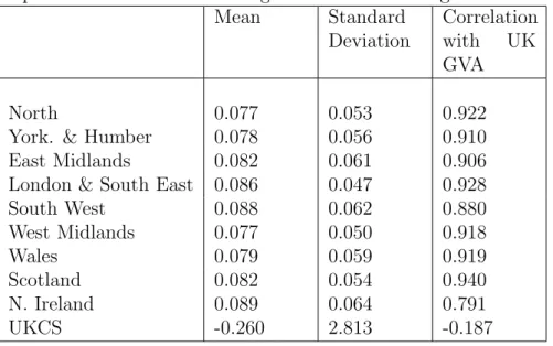
In this paper we use entropic tilting since we expect the cross-sectional restriction to hold only approximately and, thus, we do not wish to impose it exactly as in (“hard”) condi-tional forecasting (or least squares methods). In our case, this cross-seccondi-tional relationship is approximate since the GVA data for the regions that we use do not exactly add up to UK GVA because of measurement error (see the Data Appendix) and because our main results exclude GVA produced in the UK continental shelf (UKCS). UKCS data are dominated by the activities of the UK oil and gas sector.

As Table 5 shows, the UKCS data exhibit volatile behaviour that is also inconsistent with how the other regions relate to UK GVA. As a result, for our main results, we do not include

UKCS in yA

t for fear of contaminating the relationship between the other UK regions and

UK GVA with potentially deleterious effects on the accuracy of the nowcasts. However, as it is ultimately an empirical matter what works best, we also present results which do include

UKCS in yA

t. In both cases, UKCS remains part of yt,qU K; i.e. the UK GVA figures that we

condition the regional nowcasts on include the UKCS. This means that for those VARs that

exclude UKCS inyA

t this is an additional reason, to measurement error, why we expect the

cross-sectional relationship to hold only approximately. Note that it is not possible to remove UKCS activity from the overall estimates of UK quarterly GVA and then entropically tilt towards that estimate. While some sectoral detail for GVA is available for the UK as a whole on a more timely basis, not all Oil and Gas related activity in the UK ‘Mining & quarrying

(13)

including oil and gas extraction’ sector is activity which takes place in the UKCS. Some of this activity relates to onshore activity in support of activity in the UKCS. Similarly, not all of the activity in this sector relates to oil and gas extraction. It would therefore not be appropriate to treat the ‘Mining & quarrying including oil and gas extraction’ sector as synonymous with the UKCS activity series.

The idea of entropic tilting is to produce a new predictive density,

p∗(yτ+1|Dataτ), which has a mean which satisfies the restriction but is in all other respects

as close as possible to p(yτ+1|Dataτ). “As close as possible” is defined according to the

Kullback-Leibler Information Criterion (KLIC) which is a measure of the relative entropy

of p∗(yτ+1|Dataτ) to p(yτ+1|Dataτ). So, in our case, the predictive mean (i.e. the point

forecast) produced byp∗(yτ+1|Dataτ) will satisfy the restrictions but otherwise the predictive

density will be as close as possible to the unrestricted predictive density produced by the stacked VAR.

We use results based on a Normal approximation. Conditional on the parameters of the model, the predictive density from our model is Normal. The unconditional predictive density integrates out the parameters and, thus, is no longer Normal but is likely to be nearly so.

Assume that the unrestricted predictive density is Normal:

yτ+1|Dataτ ∼N(µ, V) (10)

and break down the parameters into UK and regional blocks as follows:

µ= µU K µR , V = VU K VU K,R0 VU K,R VR . (11)

The estimation procedure of the preceding sub-section will provide µand V.

Now suppose that we want to tilt the multivariate predictive density so that the mean of

some variable (or set of variables) is fixed (e.g. so as to set the predictive mean of y_τU K₊₁ to

µ∗_{U K} whereµ∗_{U K} is chosen to reflect periodτ+ 1 UK-wide information that has come available

before the τ + 1 regional data are released), but otherwise we want to leave the predictive

density to be as close to p(yτ+1|Dataτ) as possible. It can be shown (see, e.g., Altavilla,

Giacomini and Ragusa, 2017) that the tilted predictive density is:

y∗_τ₊₁|Dataτ ∼N(µ∗, V∗) (12)

where V∗ =V (i.e. tilting does not change the predictive variance) and

µ∗ = µ∗_{U K} µR−VU K,RV_{U K}−1 (µU K−µ∗U K) = µ∗_{U K} µ∗_R . (13)

Note that this type of entropic tilting relates to UK variables since this is what is being released throughout the year. Thus, it may appear that it does not directly impact on the

(14)

that, unless VU K,R = 0 and the UK nowcasts are uncorrelated with the regional nowcasts,

the updating of UK GVA nowcasts will spill over into the regional nowcasts. Note that

cross-region dependencies are captured viaVR.

But we also want to tilt toward the cross-sectional constraint which does directly relate to the regional growth nowcasts. To add the latter restriction, we extend the conventional

result given in (12). To this end, we define a new variablez =Ayt+1. The properties of the

multivariate Normal distribution imply

z ∼N(Aµ, AV A0) (14)

for any M×N matrix A. If we set

A= w IN (15)

where w = (0,0,0,0, w1,t−1, .., wR,t−1) and wr,t−1 for r = 1, .., R are region-specific weights

to be defined below, then z contains the weighted average of the nowcasts of regional GVA

growth as its first element, followed by the four quarterly UK GVA growth nowcasts, followed

by theR regional nowcasts.

We apply the entropic tilting formula of (12) to z. To this end, let µ† = Aµ and V† =

AV A0 where µ†= µ†₁ µ†₂ , V† = V₁₁† V₂₁†0 V₂₁† V₂₂† (16)

and assume that the tilting restrictions are µ†₁ = µ∗₁. Let z† denote the tilted version of z.

Then the same derivations used to find (12) can be used to show that:

z‡ ∼N µ‡, V† (17) where µ‡= " µ∗₁ µ†₂−V₂₁†V₁₁†−1µ†₁−µ∗₁ # . (18)

Note that V† will be a singular matrix, but this causes no problem for our derivations

as they only involve inverting V₁₁† (which is non-singular) and we are only interested in the

tilted predictive densities for the regional GVA variables which have predictive covariance

matrix V₂₂† (which is non-singular).

The preceding material described the general motivation and formulae relating to entropic

tilting. To describe the precise way we implement it (i.e. the exact choice for µ∗₁), we first

define the temporal and cross-sectional constraints we will use. These results arise from the

fact that annual UK GVA, YU K

t , can be written in two different ways:

Y_tU K = 4 X q=1 Y_t,qU K = R X r=1 Y_tr,A. (19)

(15)

In growth rates, this implies y_tU K = Y U K t −YtU K−1 YU K t−1 = 4 X q=1        Y_tU K₋₁_,q 4 X q=1 YU K t−1,q        yU K_t,q (20) = R X r=1       Y_tr,A₋₁_,q R X r=1 Y_tr,A₋₁_,q       y_tr,A = 4 X q=1 wuk_q,t₋₁yU K_t,q = R X r=1 wr,t−1y r,A t

whereyU K_t,q is UK growth relative to the previous year and thew’s are the weights.

Now imagine we know yU K

t+1,1 i.e. UK growth in the first quarter of year (t+ 1). We wish

to impose this information when nowcasting, but yU K

t+1,2, ytU K+1,3, ytU K+1,4 are still unknown. We

therefore assume, when tilting to reflect the cross-sectional constraint, that y_tU K₊₁_,₂ =y_tU K₊₁_,₃ =

yU K

t+1,4 = ytU K+1,1 i.e. growth continues through year t+ 1 at the rate seen in the first quarter.

Given that our data are seasonally adjusted, the assumption of constant growth throughout the year is the most reasonable one and, as we shall see, it works well empirically. This implies we tilt to reflect

y_tU K₊₁_,₁ =

R

X

r=1

wr,tyr,At+1. (21)

Now assume we know yU K

t+1,1 and ytU K+1,2 and again assume growth continues at the most

recent quarterly rate through the remainder of the year. This means we now tilt to reflect:

w₁uk_,ty_tU K₊₁_,₁ + 3wuk₂_,tyU K_t₊₁_,₂= R X r=1 wr,ty r,A t+1. (22)

Noting that the first element of µ∗₁ will relate to the variable

R

X

r=1

wr,tyr,At+1, the following

summarises how we proceed as we update our nowcasts using entropic tilting as new UK

data (Q1 to Q4, i.e. yU K

τ+1,1 toyU Kτ+1,4) are released:

1. After the release of Q1 UK GVA growth (in May of each year) set:

µ∗₁ = yU K

τ+1,1, yU Kτ+1,1

0

(16)

2. After Q2 release (in August of each year) set:

µ∗₁ = wuk₁_,τy_τU K₊₁_,₁+ 3wuk₂_,τy_τU K₊₁_,₂, y_τU K₊₁_,₁, yU K_τ₊₁_,₂0. 3. After Q3 release (in November of each year) set:

µ∗₁= wuk 1,τyτU K+1,1+wuk2,τyτU K+1,2+ 2w3uk,τyτU K+1,3 , yU K τ+1,1, yτU K+1,2, yτU K+1,3 0 . 4. After Q4 release (in February of each year) set:

µ∗₁ = yU K

τ+1, yτU K+1,1, yτU K+1,2, yU Kτ+1,3, yU Kτ+1,4

0

.

In fact, since prior to release of the Q4 data for yearτ + 1 the regional GVA data for year τ

are not yet available (since 2005 the regional data have been published in December of each year), and so as to respect this publication lag and produce genuinely real-time nowcasts, we condition our Q1 to Q3 nowcasts on 2-year rather than 1-year ahead (unconditional) density forecasts from the VARs. While this does not affect how we condition the regional nowcasts

on within-year (τ + 1) data for the UK, as detailed in 1. to 4. above, for the Q1 to Q3

nowcasts we consider an augmented A matrix and an augmented µ† vector, see (23) below,

that let us impose the additional cross-sectional constraint that the regional data for yearτ,

while now forecast rather than assumed known as in Q4, are consistent with known UK data

for (the previous) yearτ that are available from when the Q1 nowcast is made for yearτ+ 1.

A=                     0 0 0 0 0 0 0 0 w_τ0₋₁ 01×R 1 0 0 0 0 0 0 0 01×R 01×R 0 1 0 0 0 0 0 0 01×R 01×R 0 0 1 0 0 0 0 0 01×R 01×R 0 0 0 1 0 0 0 0 01×R 01×R 0 0 0 0 0 0 0 0 01×R wτ0 0 0 0 0 1 0 0 0 01×R 01×R 0 0 0 0 0 1 0 0 01×R 01×R 0 0 0 0 0 0 1 0 01×R 01×R 0 0 0 0 0 0 0 1 01×R 01×R 0 0 0 0 0 0 0 0 IR 0R 0 0 0 0 0 0 0 0 0R IR                                     yU K_τ,₁ yU K_τ,₂ yU K τ,3 yU K τ,4 yU K τ+1,1 yU K τ+1,2 yU K τ+1,3 yU K τ+1,4 yA τ y_τA₊₁                 ; µ†=                     yU K τ y_τ,U K₁ y_τ,U K₂ yU K τ,3 yU K τ,4 yU K τ+1 yU K τ+1,1 yU K τ+1,2 yU K_τ₊₁_,₃ yU K_τ₊₁_,₄ y_τA yA τ+1                     (23)

3 Empirical Results

In this section, we examine the performance of our nowcasting methods using data from 1967-2016. We continue to use quarterly UK GVA growth data and annual GVA growth data for either 9 UK regions or 10 if we include UKCS; i.e. we continue to focus in these

baseline empirical results on stacked VAR models inyt, as defined in equation (1), before we

turn to consideration of larger VAR models, with additional indicator variables, in section 3.1 below.

(17)

Figure 1: GVA Growth for the UK Regions (in %: 100×y_tr,A) 1970 1975 1980 1985 1990 1995 2000 2005 2010 2015 Year -5 0 5 10 15 20 25 30 35 Percentage North

Yorkshire & Humber East Midlands London & SE South West West Midlands Wales Scotland Northern Ireland UK

Definitions of these regions and further details of the data are given in the Data Appendix. It is worth reiterating that in this empirical exercise we use, as closely as possible, first release GVA estimates in our model, and compare our nowcasts to these same data (plotted in Figure 1). In this way our empirical exercise is as near as possible real-time. The key question of interest is whether the entropic tilting using timely, quarterly, UK-wide data will improve the nowcasts of (ONS first release) regional GVA data. This is the question we will focus on in this section To evaluate the nowcasts from the VAR models, we use a variety of standard measures of forecast performance. In particular, we use root mean squared forecast errors (RMSFE) to evaluate the quality of the point nowcasts. The evaluation of the accuracy of the entire predictive density uses log predictive scores (LPS) and the continuous ranked probability score (CRPS). See Appendix A.10 of Dieppe, Legrand, and van Roye (2016) for definitions of all these nowcast (forecast) evaluation metrics. We report these results for the VAR models relative to the (2-year ahead density) forecasts from AR(1) models (with Normal errors). These models simply take the annual regional data for each region individually and use ordinary least squares (OLS) methods; but given the aforementioned publication lags we use 2-year ahead forecasts. Comparison against a univariate benchmark enables us to assess the utility in our VAR models of conditioning the regional nowcasts on within-year UK data exploiting inter-regional dynamics. While arguably the most common forecasting benchmark in applied macroeconomics, with some attractive robustness properties in the presence of structural breaks (e.g. see Clements and Hendry, 1999), we examine the sensivity of our

(18)

results to this specific choice for the benchmark model in section 3.1 below by considering a more sophisticated mixed frequency univariate benchmark.

To aid in interpretation, note that relative values for the CRPS and RMSFE measures less than unity indicate that there are forecast gains associated with use of our VAR models; these

relative values are calculated as the CRPS or RMSFE from our nowcasting model divided by the CRPS or RMSFE from the benchmark model. For the LPS we subtract the LPS for the benchmark model from those for each of our VAR models; positive values now therefore indicate improved forecast accuracy, relative to the univariate benchmark and are similar to a Bayes factor (except that the Bayes factor is an evaluation of predictive performance over the entire sample). With Bayes factors a common rule of thumb (see Kass and Raftery, 1995) is that there is strong evidence in favour of one model over another if the log Bayes factor is greater than 3. The reader is advised to keep this value in mind when comparing LPS results from different approaches.

Our nowcast evaluation period begins in 2006. Our methods are recursive, and involve repeated re-estimation of our models. That is, we do a real-time out-of-sample nowcasting exercise using an expanding window of data beginning in 2006.

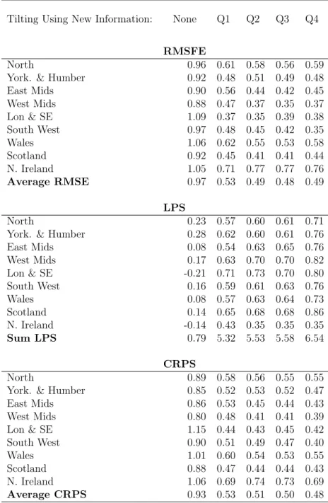
Tables 1 and 2 present these three forecast metrics, relative to the AR model, for the 9 UK regions for the homoskedastic and heteroskedastic stacked VARs. Tables 3 and 4 repeat the analysis using 10 regions, where UKCS is included in the stacked VAR. The final row of each panel of each table presents an average (for RMSFE and CRPS) or sum (for LPS) over all regions. As one moves from left to right in the tables, the forecasting metrics reflect more and more information. The first column of numbers in each table is based on unconditional nowcasts (i.e. 2-year density forecasts from the VARs). In all these tables, it can be seen that, except on one occasion if interested in nowcasting the UKCS, incorporating new information on UK GVA (as it accumulates each quarter) via our entropic tilting methods, produces more accurate nowcasts. That is, substantial decreases in RMSFEs and CRPSs and increases in LPSs, relative to the AR benchmark, are observed as we move through the year. For instance, in Table 1 we find that the average (across regions) of the RMSFEs is almost half as small by the end of the year as it was at the beginning (i.e. it drops from 0.97 to 0.49 as we move through the year). Thus, overall, the point forecasts are improving substantially. The LPS results show that similar improvements occur for the entire predictive density. For instance,

in Table 1 the sum of the LPSs over all regions increases from 0.79 to 6.54, which is strong

evidence in favour of conditioning on UK GVA values bearing in mind that log Bayes factors greater than 3 are generally seen as strong. The gains are also strong using the CRPSs with, in Table 1, the average over all regions dropping from 0.93 to 0.48 and the average CRPS dropping from 0.85 to 0.55 in Table 2. Interestingly most of the gains in nowcast performance are found after the first quarter of UK GVA data are released. Thus, nowcasts produced as early as May by our stacked VAR approach are appreciably better than the unconditional nowcasts that would have been produced in February. There are nevertheless modest gains seen, on average in Table 1, as quarterly information accrues through the year with the RMSE

(19)

and CRPS ratios declining and the LPS differences increasing. Interestingly, conditioning on the Q4 release does not help much; this is despite the fact that it is only with this Q4 release of UK GVA that the regional data for the previous year become available, so that we can condition on a 1 rather than a 2-year (unconditional) density forecast from the VAR.

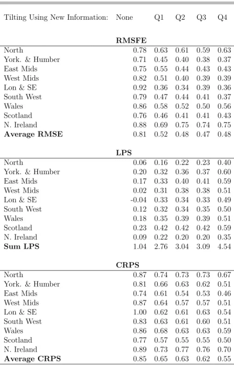
The fact that our four tables are producing similar results offers reassurance that our results are robust to changes in specification and in data. We note that there is little evidence that inclusion of stochastic volatility is important in this application, perhaps related to our use of yearly rather than higher frequency forecasts. It is true that, if we use conventional model comparison measures using the unconditional forecasts, the inclusion of stochastic volatility does lead to slight improvements relative to the homoskedatic model. For instance, the sum of the log predictive scores is 1.04 in Table 2 (which includes stochastic volatility) and 0.79 in Table 1 (which does not). A similar pattern can be found if we compare Tables 3 and 4. However, when we look at the entropically tilted nowcasts, the homoskedastic version of the model tends to do better. For instance, the sum of log predictive scores using tilted nowcasts with 4 quarters of UK GVA growth is 6.54 in Table 1 but only 4.54 in Table 2.

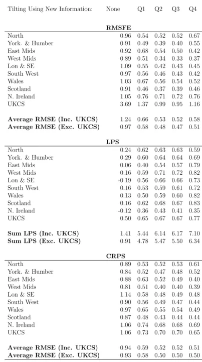
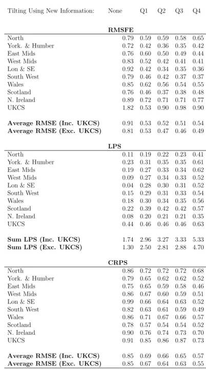
A comparison of Tables 3 and 4 with Tables 1 and 2 indicates that including UKCS as a region does not tend (with a few exceptions) to lead to any improvements in nowcast performance for the 9 other UK regions. For instance, the best overall summary of evidence is probably the sum of the log predictive scores for the 9 UK regions; and for this a comparison of Table 1 and Table 3 indicates that including UKCS leads to a rise of 0.12 in the unconditional forecast case, but reductions in the log predictive scores across the other four nowcasts (relative to the AR benchmark). On this basis, we conclude that omitting UKCS is not harmful and take the homoskedastic mixed frequency VAR with nine regions as being our preferred specification to look at in more detail. We are not surprised by this result, given the distinct (univariate) time series properties of UKCS relative to the other regions of the UK as summarised in Table 5.

If we look at the individual regions, they uniformly exhibit the same patterns noted above. As new information about UK GVA is released (on a quarterly basis) it clearly is helping to improve nowcasts for every region. These (relative) nowcast improvements are particularly large for London and the South East. This is not surprising, since this region comprises a large share of UK GVA; and, as Table 5 shows, it is (in-sample) the most correlated English region with UK GVA growth. Following Pesaran (2006), UK GVA growth - as a cross-sectional average - can be interpreted as the common “factor” driving regional growth dynamics. But even for smaller regions (e.g. Scotland), we find nowcast improvements which are similarly large. This is consistent with these regions’ growth dynamics still being dominated by (com-mon) UK dynamics, again as illustrated via the high correlations of regional GVA growth with UK GVA growth shown in Table 5. The weakest relative performance is for Northern Ireland. As seen in Table 5, GVA growth in Northern Ireland exhibits the lowest correlation with UK GVA at 0.8 compared with at least 0.9 for the other regions (with the exception of the UKCS). This suggests that GVA movements in Northern Ireland depend less on the

(20)

common UK “factor” than in the other regions of the UK. But even for Northern Ireland, the nowcast metrics improve as new information on UK GVA growth is incorporated throughout the year; and the nowcasts are clearly more accurate than those from the AR benchmark (with gains of at least 20% across the three evaluation metrics).

It can be seen that while there are often gains from using an unconditional multivariate forecasting method which allows information from different regions and the UK as a whole to inform the forecasts of a particular region, our unconditional forecasting metrics (i.e. without entropic tilting) do not always beat the AR(1) benchmark. London and the South East is a leading example in Table 1. It is only when entropic tilting is used that we see the more substantive gains. That is, when we use the additional quarterly UK data as it released throughout the year large gains are made relative to a simple univariate method.

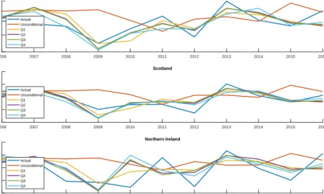
Tables 1 to 4 reflect average performance over our nowcast evaluation period. Figures 2 to 4 shed light on whether there are particular time periods when incorporating new in-formation using our tilting methods is particularly important. These figures are based on the homoskedastic mixed frequency stacked VAR and do not include the UKCS. They plot, for each region, actual regional GVA growth (i.e. the subsequent realisation using the first estimate from the ONS) along with our five different nowcasts (conditional means of the now-cast densities). One clear pattern which emerges, to varying degrees across regions, is that 2009 is a year where updating regional nowcasts, in the light of the more timely UK data, is particularly important. As the Great Recession hit, the unconditional forecast of 2009 GVA growth turned out to be much higher than the realisation in every region. However, our tilting methodology quickly downgraded the 2009 nowcasts. 2013 is another year when the tilted nowcasts showed big improvements relative to the unconditional forecasts. In this case, realised GVA growth in all regions was higher than expected and the unconditional forecast was too low in every region. By tilting towards UK-wide releases as they came available, the nowcasts were upgraded and ended up being much closer to the actual 2013 realisation.

3.1 Robustness

3.1.1 Larger VAR models

In other nowcasting and forecasting applications, albeit of aggregate output growth, it has been found that consideration of a larger set of indicators can be beneficial; e.g. see Banbura, Giannone, Reichlin (2010), Foroni and Marcellino (2014) and Carriero, Clark and Marcellino (2015). Similarly, in our application, we might hope that additional indicators help explain and anticipate regional output growth. It is ultimately an empirical matter. But we should

admit that we are (a priori) somewhat cautious about the predictive content of these

ad-ditional indicators, given that they do not share the characteristic of UK GVA growth, the main indicator considered above, of being the cross-sectional aggregation of the regional GVA data that we are in fact seeking to nowcast.

(21)

nowcasts when additional quarterly and/or annual indicators, at the regional, sectoral and aggregate levels, are included in our VAR models, in this section we provide some evidence that evaluates how nowcast accuracy is affected empirically when we do consider some stacked VAR models augmented with additional indicators. We should emphasise that our stacked VAR models are already pretty ‘large’, given our consideration of regional data, and of a comparable size to the ‘large’ VAR models considered, for example, in Carriero, Clark and Marcellino (2015)’s nowcasting application. So consideration of appreciably larger VAR mod-els raises computational challenges, given our model specification and strategy to estimate the shrinkage parameters preclude use of analytical methods. We therefore restrict our attention to VAR models with a dozen or so additional indicators.

Our experiments involved adding to yt candidate indicator variables that might credibly

be believed to offer some additional (to quarterly UK GVA growth and lagged regional GVA growth) explanatory power for regional GVA growth. In searching for these indicator variables, inevitably we face some data constraints and limitations. In applications which nowcast country-wide output growth, timely data on industrial production are often found to improve accuracy (e.g. see Mazzi, Mitchell and Montana, 2014). However, the ONS do not publish higher-frequency and/or more timely breakdowns of regional industrial production. Drawing on Bell, Co, Stone and Wallis (2014) in their application which nowcasts (aggregate) output growth in the UK, we might also hope to use qualitative business survey data, as they find these survey data are useful and timely indicators of UK output growth. While regional breakdowns of these business survey data, for example PMI data, are available, in fact at the monthly frequency, their historical coverage is limited; regional PMI data date back to 1997 only. But the historical coverage of regional labour market data is better. So we do augment our stacked VAR model with regional data on jobseeker’s allowance (JSA), an ONS measure of unemployment. JSA data are in fact available monthly, but we choose to work with them aggregated to the quarterly frequency. But in aggregating we accommodate the fact that these JSA data are currently released just two weeks after the end of the month of

interest. So, for example, in definingytwe match the JSA annual growth rate ending in April

(published in May) with the Q1 UK GVA growth estimates,yU K_t,₁ , that also become available

in May. Similarly, the Q2 data, yU K

t,2 , are matched to JSA annual growth rates ending in

July, and so on for the other quarters. These regional JSA data, which are not typically revised so we use latest vintage data, date back to 1975; we backcast earlier estimates using the UK aggregate. We also add to our VAR model sectoral GVA growth data: for the service sector, manufacturing, construction and agriculture. These data are released at the same time as the quarterly UK GVA data; with historical data available from the Bank of England’s real-time database. As the sectoral composition of the UK regions varies, we might find that regional output growth is better explained by sectoral rather than total output growth. Consideration of these extra indicators at the quarterly frequency would increase

the dimension of our stacked VAR model by (9 + 4)×4. To facilitate computation, but after

(22)

VAR by including only the Q4 values of these additional indicators; these are always, in any case, the latest estimates known when the unconditional predictive densities are recursively computed. However, when tilting we do so conditioning on the latest quarterly estimate of annual growth available for that indicator at each of the four points within the year at which we update the nowcasts.

Accordingly, we repeated the real-time out-of-sample nowcasting exercise above using this larger VAR model (as discussed, having also experimented with alternatives, dropping or including subsets of these additional indicators, and finding results to be similar). Table 6 reports results, continuing to focus on the homoskedastic stacked VAR that does not include the UKCS - given this was found to be the preferred model above. Comparing Tables 1 and 6 we are therefore able to evaluate the empirical utility of using the larger set of indicators. Looking first at the accuracy of the unconditional forecasts, we see little evidence to suggest that the larger set of indicator delivers improved accuracy; this is so irrespective of which of the three measures of forecast performance we consult. In fact, it is striking how similar accuracy is across Tables 1 and 6 when confining attention to the unconditional forecasts; if anything the slight edge goes to the smaller VAR in Table 1. But when we turn to look at the conditional nowcasts, we find the larger VAR model to be outperformed by the smaller VAR model. This is especially so when measures of density accuracy are consulted. The CRPS and LPS statistics are clearly worse than for the smaller model - even when we condition on the Q4 release. Inspection of the underlying density nowcasts from the larger VAR models (not reported) indicates this may be explained by the extra uncertainty apparently associated when nowcasting with this larger set of indicators; the variances of the predictive nowcasts are often double those from the smaller VAR model, with the extra parameter estimation error associated with the larger VAR model no doubt contributing to this. An explanation for these results is that, in contrast to other relationships in the larger VAR model, there is a more stable relationship between UK output growth and regional output growth. These other indicators offer little or no, given their noise, value-added relative to conditioning the regional nowcasts on UK-wide output growth (and lagged values).

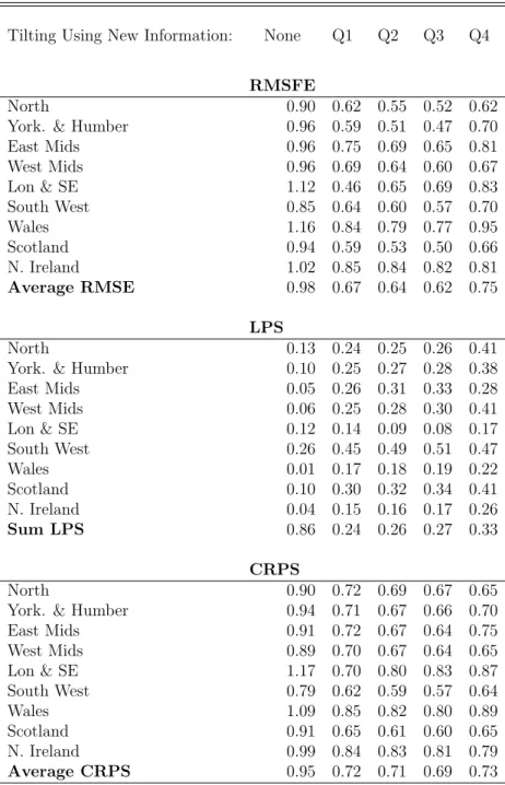
3.1.2 A mixed frequency (MIDAS) benchmark

To assess the incremental gains of entropic tilting and imposing the cross-sectional constraint on our cross-region stacked VAR model, we also compare our results with those from a mixed frequency univariate benchmark model that allows the regional nowcasts to be updated through the year as the quarterly UK GVA data are released. To accommodate the fact that this benchmark model now conditions on available quarterly UK GVA data, and is therefore mixed frequency, we follow Foroni, Marcellino and Schumacher (2015) and, in effect, use “Unrestricted” U-MIDAS models. These involve recursively forecasting using regressions of annual regional GVA growth on lagged (again by two years) growth, as with the AR benchmark, but then adding Q1-Q4 quarterly UK GDP as (an) additional indicator(s). So while the first (Q1) nowcast, produced before the first release of Q1 UK GVA growth, is the

(23)

same as the nowcast produced from the AR, the second nowcast also conditions on current year Q1 UK GVA growth, the third nowcast on both Q1 and Q2 UK GVA growth, and so on.

We construct the density nowcasts from these U-MIDAS models analytically, assuming normality for the errors, with the variance of the density nowcast computed to account for parameter estimation uncertainty as suggested by Clements and Galvao (2017); for a more general discussion see Aastveit, Foroni and Ravazzolo (2017). We should note that accommodating parameter estimation error does little to affect the AR results considered in Tables 1 to 4 above; but for these less parsimonious U-MIDAS models it does make a difference.

Table 7 reports the RMSE, CRPS and LPS statistics from these U-MIDAS models relative to those from the AR; with numbers less than unity, for RMSE and CRPS, again indicating that the U-MIDAS model is more accurate; and numbers for LPS greater than zero indicating that the U-MIDAS model is more accurate. Looking at RMSE first, for several regions, but a decreasing number as we move right in the tables, U-MIDAS is better. But looking at the measures of density accuracy, we see overwhelming evidence that the U-MIDAS models are less accurate than the arguably more naive AR benchmark. This result is less surprising when we note that the U-MIDAS models, as they condition on accumulating within-year (Q1-Q4) UK GVA growth data fit the regional GVA growth data increasingly well in-sample - as within-year data accumulates. The in-sample fit of these regressions is considerably higher than those of the AR benchmark. This in-sample accuracy then translates into narrower pre-dictive nowcasts for regional GVA growth, notwithstanding some extra parameter estimation error as the U-MIDAS models are less parsimonious. And given the out-of-sample ‘shocks’ evident over our out-of-sample period, these narrow density nowcasts from the U-MIDAS models often appear to miss or attach a very low probability to the subsequent regional GVA growth outturn.

4 Conclusions

In this paper we have highlighted the need for more timely macroeconomic data for the UK regions. Our desire is to produce regional GVA estimates which are more frequent (quarterly instead of annual) and also more timely. We have developed an econometric procedure which combines a mixed frequency stacked VAR with entropic tilting. Our key contributions lie in the incorporation of the new, more timely, information provided by the quarterly releases of UK wide data acknowledging the fact that UK growth is a weighted average of growth for the individual regions. Exploiting this cross-sectional constraint, and noting that we do not expect it to hold exactly, we are able to produce updated regional nowcasts to the same timescale as the ONS currently produce their quarterly UK estimates. That is, the latest UK data help allocate national growth among the regions of the UK. In a real-time nowcasting exercise we find our methods to work well. As new, quarterly UK wide information is released throughout

(24)

the year our nowcasts of regional GVA growth improve. Thus, using the methods we propose, regional policymakers can have at their disposal more accurate nowcasts of current growth rates. They do not have to rely on out-of-date figures or indeed have to wait many months for new regional data releases from ONS.

We hope that entropic tilting, with mixed frequency stacked VARs, as developed in this paper will find other applications when interested in nowcasting and forecasting with data subject to aggregation constraints and differential publication lags.

(25)

Table 1: Nowcasting Performance Using Homoskedastic Mixed Frequency VAR (Results

Relative to AR Benchmark)Note: the RMSFE and CRPS values from our VAR nowcasting

model are presented relative to (divided by) those from the benchmark AR model; in the same way the LPS are presented relative to (by subtraction of ) the LPS from the AR model.

Tilting Using New Information: None Q1 Q2 Q3 Q4

RMSFE

North 0.96 0.61 0.58 0.56 0.59 York. & Humber 0.92 0.48 0.51 0.49 0.48 East Mids 0.90 0.56 0.44 0.42 0.45 West Mids 0.88 0.47 0.37 0.35 0.37 Lon & SE 1.09 0.37 0.35 0.39 0.38 South West 0.97 0.48 0.45 0.42 0.35 Wales 1.06 0.62 0.55 0.53 0.58 Scotland 0.92 0.45 0.41 0.41 0.44 N. Ireland 1.05 0.71 0.77 0.77 0.76 Average RMSE 0.97 0.53 0.49 0.48 0.49 LPS North 0.23 0.57 0.60 0.61 0.71 York. & Humber 0.28 0.62 0.60 0.61 0.76 East Mids 0.08 0.54 0.63 0.65 0.76 West Mids 0.17 0.63 0.70 0.70 0.82 Lon & SE -0.21 0.71 0.73 0.70 0.80 South West 0.16 0.59 0.61 0.63 0.76 Wales 0.08 0.57 0.63 0.64 0.73 Scotland 0.14 0.65 0.68 0.68 0.86 N. Ireland -0.14 0.43 0.35 0.35 0.35 Sum LPS 0.79 5.32 5.53 5.58 6.54 CRPS North 0.89 0.58 0.56 0.55 0.55 York. & Humber 0.85 0.52 0.53 0.52 0.47 East Mids 0.86 0.53 0.45 0.44 0.43 West Mids 0.80 0.48 0.41 0.41 0.39 Lon & SE 1.15 0.44 0.43 0.45 0.42 South West 0.90 0.51 0.49 0.47 0.40 Wales 1.01 0.60 0.54 0.53 0.55 Scotland 0.88 0.47 0.44 0.44 0.43 N. Ireland 1.06 0.69 0.74 0.73 0.69 Average CRPS 0.93 0.53 0.51 0.50 0.48

(26)

Table 2: Nowcasting Performance Using Mixed Frequency VAR with Stochastic Volatility

(Results Relative to AR Benchmark) Note: the RMSFE and CRPS values from our VAR

nowcasting model are presented relative to (divided by) those from the benchmark AR model; in the same way the LPS are presented relative to (by subtraction of ) the LPS from the AR model.

RMSFE

North 0.78 0.63 0.61 0.59 0.63 York. & Humber 0.71 0.45 0.40 0.38 0.37 East Mids 0.75 0.55 0.44 0.43 0.43 West Mids 0.82 0.51 0.40 0.39 0.39 Lon & SE 0.92 0.36 0.34 0.39 0.36 South West 0.79 0.47 0.44 0.41 0.37 Wales 0.86 0.58 0.52 0.50 0.56 Scotland 0.76 0.46 0.41 0.41 0.43 N. Ireland 0.88 0.69 0.75 0.74 0.75 Average RMSE 0.81 0.52 0.48 0.47 0.48 LPS North 0.06 0.16 0.22 0.23 0.40 York. & Humber 0.20 0.32 0.36 0.37 0.60 East Mids 0.17 0.33 0.40 0.41 0.59 West Mids 0.02 0.31 0.38 0.38 0.51 Lon & SE -0.04 0.33 0.34 0.33 0.49 South West 0.12 0.32 0.34 0.35 0.50 Wales 0.18 0.35 0.39 0.39 0.51 Scotland 0.23 0.42 0.42 0.42 0.59 N. Ireland 0.09 0.22 0.20 0.20 0.35 Sum LPS 1.04 2.76 3.04 3.09 4.54 CRPS North 0.87 0.74 0.73 0.73 0.67 York. & Humber 0.81 0.66 0.63 0.62 0.51 East Mids 0.74 0.61 0.54 0.53 0.46 West Mids 0.87 0.64 0.57 0.57 0.51 Lon & SE 1.00 0.62 0.61 0.63 0.54 South West 0.83 0.63 0.61 0.60 0.51 Wales 0.86 0.68 0.63 0.63 0.59 Scotland 0.77 0.57 0.55 0.55 0.50 N. Ireland 0.89 0.73 0.77 0.76 0.70 Average CRPS 0.85 0.65 0.63 0.62 0.55

(27)

Table 3: Nowcasting Performance Using Homoskedastic Mixed Frequency VAR including

UKCS (Results Relative to AR Benchmark)Note: the RMSFE and CRPS values from our

VAR nowcasting model are presented relative to (divided by) those from the benchmark AR model; in the same way the LPS are presented relative to (by subtraction of ) the LPS from the AR model.

RMSFE

North 0.96 0.54 0.52 0.52 0.67

York. & Humber 0.91 0.49 0.39 0.40 0.55

East Mids 0.92 0.68 0.54 0.50 0.42 West Mids 0.89 0.51 0.34 0.33 0.37 Lon & SE 1.09 0.55 0.42 0.43 0.45 South West 0.97 0.56 0.46 0.43 0.42 Wales 1.03 0.67 0.56 0.54 0.52 Scotland 0.91 0.46 0.37 0.39 0.46 N. Ireland 1.05 0.76 0.71 0.72 0.76 UKCS 3.69 1.37 0.99 0.95 1.16

Average RMSE (Inc. UKCS) 1.24 0.66 0.53 0.52 0.58

Average RMSE (Exc. UKCS) 0.97 0.58 0.48 0.47 0.51

LPS

North 0.24 0.62 0.63 0.63 0.59

York. & Humber 0.29 0.60 0.64 0.64 0.69

East Mids 0.06 0.40 0.54 0.57 0.79 West Mids 0.16 0.59 0.71 0.72 0.82 Lon & SE -0.19 0.56 0.66 0.66 0.73 South West 0.16 0.53 0.59 0.61 0.72 Wales 0.13 0.50 0.59 0.60 0.82 Scotland 0.16 0.62 0.68 0.67 0.83 N. Ireland -0.12 0.36 0.43 0.41 0.35 UKCS 0.50 0.65 0.67 0.67 0.77

Sum LPS (Inc. UKCS) 1.41 5.44 6.14 6.17 7.10

Sum LPS (Exc. UKCS) 0.91 4.78 5.47 5.50 6.34

CRPS

North 0.89 0.53 0.52 0.53 0.61

York. & Humber 0.84 0.52 0.47 0.48 0.52

(28)

Table 4: Nowcasting Performance Using Mixed Frequency VAR with Stochastic Volatility

and including UKCS (Results Relative to AR Benchmark) Note: the RMSFE and CRPS

values from our VAR nowcasting model are presented relative to (divided by) those from the benchmark AR model; in the same way the LPS are presented relative to (by subtraction of ) the LPS from the AR model.

RMSFE

North 0.79 0.59 0.59 0.58 0.65

York. & Humber 0.72 0.42 0.36 0.35 0.42

Average RMSE (Exc. UKCS) 0.81 0.53 0.47 0.46 0.49

LPS

North 0.11 0.19 0.22 0.23 0.41

York. & Humber 0.23 0.31 0.35 0.35 0.61

Sum LPS (Inc. UKCS) 1.74 2.96 3.27 3.33 5.33

Sum LPS (Exc. UKCS) 1.30 2.50 2.81 2.88 4.70

CRPS

North 0.86 0.72 0.72 0.72 0.68

York. & Humber 0.79 0.65 0.62 0.62 0.52