Michael Wibral1*, Nicolae Pampu2, Viola Priesemann3, Felix Siebenhu¨hner1,4, Hannes Seiwert1, Michael Lindner5, Joseph T. Lizier6,7, Raul Vicente1,3,8
1MEG Unit, Brain Imaging Center, Goethe University, Frankfurt, Germany,2Center for Cognitive and Neural Studies (Coneural), Cluj-Napoca, Romania,3Frankfurt Institute for Advanced Studies (FIAS), Goethe University, Frankfurt, Germany,4Department of Physics, University of California Santa Barbara, Santa Barbara, California, United States of America,5Center for Economics and Neuroscience, Friedrich-Wilhelms University, Bonn, Germany,6Max Planck Institute for Mathematics in the Sciences, Leipzig, Germany,7CSIRO Information and Communication Technologies Centre, Marsfield, New South Wales, Australia,8Max-Planck Institute for Brain Research, Frankfurt, Germany
Abstract
In complex networks such as gene networks, traffic systems or brain circuits it is important to understand how long it takes for the different parts of the network to effectively influence one another. In the brain, for example, axonal delays between brain areas can amount to several tens of milliseconds, adding an intrinsic component to any timing-based processing of information. Inferring neural interaction delays is thus needed to interpret the information transfer revealed by any analysis of directed interactions across brain structures. However, a robust estimation of interaction delays from neural activity faces several challenges if modeling assumptions on interaction mechanisms are wrong or cannot be made. Here, we propose a robust estimator for neuronal interaction delays rooted in an information-theoretic framework, which allows a model-free exploration of interactions. In particular, we extend transfer entropy to account for delayed source-target interactions, while crucially retaining the conditioning on the embedded target state at the immediately previous time step. We prove that this particular extension is indeed guaranteed to identify interaction delays between two coupled systems and is the only relevant option in keeping with Wiener’s principle of causality. We demonstrate the performance of our approach in detecting interaction delays on finite data by numerical simulations of stochastic and deterministic processes, as well as on local field potential recordings. We also show the ability of the extended transfer entropy to detect the presence of multiple delays, as well as feedback loops. While evaluated on neuroscience data, we expect the estimator to be useful in other fields dealing with network dynamics.
Citation:Wibral M, Pampu N, Priesemann V, Siebenhu¨hner F, Seiwert H, et al. (2013) Measuring Information-Transfer Delays. PLoS ONE 8(2): e55809. doi:10.1371/ journal.pone.0055809
Editor:Satoru Hayasaka, Wake Forest School of Medicine, United States of America ReceivedAugust 12, 2012;AcceptedJanuary 2, 2013;PublishedFebruary 28, 2013
Copyright:ß2013 Wibral et al. This is an open-access article distributed under the terms of the Creative Commons Attribution License, which permits unrestricted use, distribution, and reproduction in any medium, provided the original author and source are credited.
Funding:MW, RV, and VP received financial support from LOEWE Grant ‘‘Neuronale Koordination Forschungsschwerpunkt Frankfurt(NeFF).’’ VP received financial support from the Max Planck Society. MW thanks the Max Planck Institute for Mathematics in the Sciences for funding a visit which contributed to this work. JL thanks the LOEWE Grant ‘‘Neuronale Koordination Forschungsschwerpunkt Frankfurt(NeFF)’’ for funding a visit which contributed to this work. The funders had no role in study design, data collection and analysis, decision to publish, or preparation of the manuscript.
Competing Interests:The authors have declared that no competing interests exist. * E-mail: [email protected]
Introduction
Many phenomena in the world around us, such as traffic systems, gene regulatory networks, neural circuits and the Internet can be best understood in terms of complex networks. Under-standing such networks requires knowledge about the existence and direction of the interactions in the network. Often, the network function also depends on the interaction timing. For example, understanding of the railway system is incomplete if only the location of train tracks and the direction in which they are used is known. At least information on train travel times is necessary to catch a glimpse of how the network serves its purpose, and only a timetable enables one to use this network efficiently. As in this example, interaction delays may have a pivotal role in under-standing the function of complex networks.
In neuroscience, interaction delays arise mainly due to propagation of action potentials (‘spikes’) along axonal processes and can amount to several tens of milliseconds. The presence of axonal delays is of particular importance for coordinated neural activity (e.g. synchronization, Hebbian learning) because they add an intrinsic component to the relative timing between spikes. For
example, two neurons projecting to a downstream neuron will be observed to spike simultaneously by this downstream neuron only when their relative timing of spikes compensates the difference in their axonal delays and in the dendritic delays to the soma of the target neuron. Indeed, disruption of coordinated activity by the pathological modification of axonal delays is thought to account for some deficits in diseases such as multiple sclerosis [1], schizophrenia [2], and autism [3]. Thus, the estimation of both, interaction delays and interaction strengths from multichannel brain recordings are needed to better resolve the dynamic coordination between different areas. In this paper we propose an extension of an information-theoretic functional, transfer entropy, to determine both the information transfer and interac-tion delays between processes.
In the following, we review the key concepts of Wiener causality and transfer entropy, and describe the outline of the paper.
Causality, Transfer Entropy, and the Estimation of Interaction Delays
Ideally, in explorative analyses both the presence of directed interactions between two physical systems, as well as their timing
should be detected without anya prioriknowledge of the coupled systems or their specific interaction mechanism, i.e. a model free analysis is required. To keep our analysis as model-free as possible, we assume that the coupled physical systems X,Y produce the observed time seriesfx1,. . .,xTg,fy1,. . .,yTgvia measurements at discrete times t[1:::T. These time series are understood as realizations xt,yt of stationary random processes X,Y for mathematical treatment. The stationarity assumption for the random processes is convenient here as it allows to replace ensemble averages by time averages, but the proposed method will also work for ensemble averaging. In the remainder of the text, upper case lettersX,Y refer to these random processes,Xt,Ytto the random variables the processes are composed of, while lower case letters with subscript indicesxt,ytrefer to scalar realizations of these random variables. Bold case lettersX,Y,Xt,Yt,xt,ytrefer to the corresponding processes, random variables, and their realiza-tions in a state space representation (see the methods section for the construction of these state spaces).
The structure of directed interactions can be analyzed by assigning a causal influence from a processXto another oneY, if knowledge about the past of realizations of X and Y together allows one to predict the future ofYbetter than knowledge about the past ofY alone. This is known as Norbert Wiener’s principle of `causality’, and does not by itself entail a modeling approach. Although this principle paved the way for a formal analysis of directed interactions, we note that today for an analysis of truly causal interactions more stringent requirements have to be met [4,5]. If only Wiener’s principle is met, we speak of predictive information transfer [6]. However, predictive information transfer may often be exactly the quantity of interest when analyzing directed interactions in networks, especially when these networks actively process information [6,7].
Wiener’s principle can be directly translated into an informa-tion-theoretic framework by reformulating it as the question: ‘‘What information does the past ofXprovide about the future ofY, that the past of Y did not already provide?’’. Schreiber [8] formalized this question in terms of a conditional mutual information I(:;:D:)
between the involved quantities: TE(X?Y)~I(Yz
;X{DY{), ð1Þ whereYz
is a future random variable of the processY, whereas X{andY{denote suitably reconstructed paststate variablesof the processesXandY, respectively. The corresponding quantity has been described several times in the literature (e.g. [8,9]) and is most often refered to astransfer entropy[8].
The use of transfer entropy or related methods [10,11] for model free analyses of directed interactions has seen a dramatic surge of interest recently, both in neuroscience [9,12–31], physiology [32–34], as well as in the general theories of computation [7,24,35] and causality [5]. For specific application scenarios transfer entropy has proven to be clearly superior compared to alternative analyses of interactions [22].
Schreiber originally defined the transfer entropy functional for random processesX andY, with discrete-valued time indext, as [8]:
TE(X?Y)~I(Ytz1;XtDYt), ð2Þ
Yet, it was noted early on that in real world physical systems information fromXneeds a finite timedto arrive atY. Because of this, past states variablesXt,Ytand future future random variables
Ytz1, that replace the abstract quantitiesX
{
,Y{andYz in the functional from equation 1 in the calculation of a specific estimator, such as in equation 2, have to be redefined appropri-ately to reflect this fact. Therefore, two suggestions were made to adapt transfer entropy:
N
First, we and others suggested to use the following formula to take efficiently into account the possibility of a non-vanishing interaction delay [9,12,13,29],TE(X?Y,u)~I(Ytzu;XtDYt), ð3Þ where the parameteruis the time which an influence needs to propagate fromXtoY[9,12,13,29]. A scanning approach for the parameteruwas suggested to recover the delay with the largest predictive information transfer and, thereby, recover the dominant interaction delay [12].
N
Second, Pompe and Runge [36] suggested a similar scanning approach to adjust the TE to consider transfer from a previous source variable Xt to a future target variable Ytzu, while conditioning on the source state variable Ytzu{1, and additionally conditioning on the previous source state variable Xt{1:MIT(X?Y,u)~I(Ytzu;XtDYtzu{1,Xt{1), ð4Þ This measure is known as themomentary information transfer(MIT) (see Methods section part on MIT for full details). While the idea to scanuin order to maximize MIT is similar to the first approach, the conditioning on a past source state was thought to ensure that the specific delay was identified where the transferred information appeared in the source first.
While the first approach in equation 3 seems like a natural extension of transfer entropy, we will show in the next section that equation 3 violates Wiener’s principle of causality. This is because the above functional violates the requirement of an optimal self prediction from the past ofYto the future ofYthat is implicit in Wiener’s principle. In short, using a stateYtthat is not obtained immediately prior to the future Ytzu – the state one is trying to predict – ignores potentially relevant predictive information (see below for details). We will provide a simple example where the above functional (equation 3) from references [9,12,13,29] does not recover the correct interaction delay.
We will also show by counter-example that the second suggestion, the MIT, is not able to reconstruct the correct interaction delay in a simple example in the presence of memory in the source.
Therefore, we present in this study an improved transfer entropy functional that honors the requirement of an optimal self prediction and that successfully recovers the correct interaction delay. We formulate a mathematical theorem that the improved transfer entropy functional is maximal when its delay parameter coincides with the underlying interaction delay and give the corresponding proof. To further validate our approach on finite data we run extensive simulations of stochastic and deterministic delay-coupled systems. Local field potentials are also used to test the recovery of interaction delays in electrophysiological recordings.
Furthermore, we will demonstrate below that our novel approach allows to test the presence of self-feedback activity in a single recorded signal. Finally, we discuss how information about interaction delays can be used to enhance the power of effective connectivity analyses.
Results
Comparison of Transfer Entropy Functionals in Relation to Wiener’s Principle
Wiener’s principle asks for information about the future ofY that the past ofXcan providein additionto the information already provided by the past ofY. If, however, this latter information is underestimated, we may potentially obtain an erroneously high value of predictive information transfer fromXtoY. From this it follows that information provided by the past ofYto the future of Y must be estimated optimally, a fact that we will refer to as the self prediction optimality (SPO) requirement from here on. Equiva-lently, from an information-theoretic computational perspective, we can view the ‘self prediction’ as aninformation storagebyY[37], and so underestimating the information storage inY’s dynamics can lead us to overestimate the information transfer fromX toY [7,35].
For practical applications of Wiener’s principle this means that we have to guarantee an optimal self prediction at least within the limits of our respective prediction framework. For the most general case of TE where no a priori model-based knowledge can be used, this means we have to resort to model free prediction, as it is for example provided by the local predictor [38,39].
We will first show that the transfer entropy functional given in equation 3 is not self prediction optimal and then provide a new transfer entropy functional that is self prediction optimal.
To show that the functional from equation 3 is indeed not self-prediction optimal, we rewrite this equation by substituting t by t{u:
TE(X?Y,u)~I(Yt;Xt{uDYt{u): ð5Þ
We see that the self prediction of Y, or equivalently the conditioning, is done based on the stateYat timet{u. Let us define u0 as the value of the parameter u that optimizes self prediction of Yt by Yt{u0. If we now scan u in search of the maximum predictive information transfer fromXt{utoYt, we will potentially condition our mutual information on statesYt{uwith u=u0, i.e. we condition on states that are not optimal for self
prediction. This suboptimal conditioning may artificially inflate transfer entropy values in au-dependent manner. Thus, maximum transfer entropy values do not only depend on the true information flow fromXtoYand its delay, but also on the quality of the self-prediction (conditioning). As a consequence, the maximal appar-ent information transfer estimated by equation 5 may be found at values ofuthat do not represent the true delayd, and the attempt to identify the true interaction delay by maximizing predictive information transfer with the functional in equation 5 may lead to erroneous results.
From the above it follows that conditioning on the past state Yt{u should always be done with respect to the optimal state Yt{u0. Hence, a modified functional reads:
TE’(X?Y,u)~I(Yt;Xt{uDYt{u0), ð6Þ whereu0in principle would have to be identified by a model-free prediction scheme, such as the one proposed by Ragwitz and Kantz [39]. However, we can abbreviate this procedure and formally prove that u0 must be 1 sample if equation 6 is to represent a causal relationship (see next subsection). Furthermore, usingu0~1properly eliminates anyinformation storagefrom the past ofYthat could otherwise be mistaken as information transfer from
X. And finally, the use ofu0~1allows us to take a dynamical systems view of thestate transitionYt{1?Yt, and consider the TE as measuring how much information Xt{u provides about this state transition.
Result. The predictive information transfer fromX toY over a time delayuis properly captured (aligning with Wiener’s principle) by:
TESPO(X?Y,u)~I(Yt;Xt{uDYt{1): ð7Þ
This functional fulfills the self prediction optimality requirement and we chose the subscript ‘SPO’ to reflect this. We note that in the caseu~1TE(X?Y,u~1)the old estimator (equation 3 ) is equal toTESPO(X?Y,u~1)(and this equality also holds for the original formulation of the TE from equation 2 ); however, this does not hold for otheruin general and as such using equation 6 withuw1and u0=1does not satisfy Wiener’s principle. To see this, we rewrite from equation 6 : TE’(X?Y,u)~I(Yt;Xt{u,Yt{u0){I(Yt;Yt{u0), which allows us then to see explicitly that both, (1) the joint information term I(Yt;Xt{u,Yt{u0) supplied by the source and the past of the target, and (2) the information storage term I(Yt;Yt{u0), differ under the casesu0~u(old delayed TE estimator, equation 3 ) and
u0~1(new delay TE estimator, equation 7).
In the next section we provide a theorem that formally states thatTESPOis maximal when the parameteruis equal to the true interaction delayd, and give a proof. Thus,TESPOcan be used to recover an interaction delaydin coupled systems as:
d~arg max
u (TESPO(X?Y,u)): ð8Þ
A Theorem on the Identifiability of the True Delaydof an Interaction
Part of this study is a proof of the fact that the new proposed functional assumes its maximal value when the delay parameteru inTESPO (equation 7) is equal to the true delay d. The main finding can be summarized in the following theorem:
Theorem 1. For two discrete-time random processesX,Ywith a state space representation X,Y, coupled from X to Y via a non-zero delayd, TESPO(X?Y,u)~I(Yt;Xt{uDYt{1) is maximal for u~d. This
also holds in the presence of additional coupling fromYtoX.
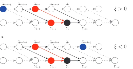
The main ideas behind delay reconstruction via maximizing TESPOare illustrated in Figure 1. By scanning the delay parameter uwe shift the considered state Xt{u of the source processX in time. If this stateXt{uis in the relative future of the observation to be predicted forY, i.e.Yt, its influence has not arrived atY yet. As a consequence, the state is uninformative and we get low TESPO. If the state has a time delayu~d, such that the influence arrives exactly atYt, thenTESPO is maximal. If the state has too long a delay, then its influence has arrived beforeYtand is already taken into account via conditioning on the past stateYt{1; again we obtain lowTESPO. In the following we will present our proof. Since it is of a technical nature the reader may safely skip ahead if not interested in this material.
Proof of Theorem 1
Outline. We start by showing that the three random variables Xt{d{j,(Xt{d,Yt{1), andYtform a Markov chain forVj=0. To this end we first demonstrate thed-separationofXt{d{jandYtby
(Xt{d,Yt{1) which is equivalent to conditional independence of Xt{d{jandYt, given(Xt{d,Yt{1)[4]. This, in turn, is equivalent
toXt{d{j?(Xt{d,Yt{1)?Ytforming a Markov chain. Using the
decomposition propertyof conditional independence (e.g. [4]), we see that this result also holds if we replace the state Yt by the corresponding scalar observation Yt. We then use this Markov chain for statements on the relation of mutual information terms
built from its variables and rearrange terms to arrive at the statements on TE formulated in theorem 1.
d-separation. From figure 2, representing the causal graph of the two random processesX,Y, we see that:
N
allsequentialpaths fromXt{d{jintoYtare blocked by the joint random variable (Xt{d,Yt{1) (sequential paths of this kind Figure 1. Illustration of the main ideas behind interaction delay reconstruction using the TESPOestimator.(A) Scalar time courses ofprocessesX,YcoupledX?Ywith delayd, as indicated by the blue arrow. Colored boxes with circles indicate data belonging to a certain state of the respective process. The star on theYtime series indicates the scalar observationY(t)to be predicted in Wiener’s sense. Three settings for the delay parameteruare depicted: (1)uvdwith – u is chosen such that influences of the stateX(t{u1)onYarrive in the future of the prediction point.
Hence, the information in this state is useless and yields no transfer entropy. (2)u~d– u is chosen such that influences of the stateX(t{u2)arrive exactly at the prediction point, and influence it. Information about this state is useful, and we obtain nonzero transfer entropy. (3)uwd– u is chosen
such that influences of the stateX(t{u3)arrive in the far past of prediction point. This information is already available in the past of the states ofY that we condition upon inTESPOInformation about this state is useless again, and we obtain zero transfer entropy. (B) Depiction of the same idea in a more detailed view, depicting states (gray boxes) ofXand the samples of the most informative state (black circles) and noninformative states (white circles). The the curve in the left column indicates the approximate dependency ofTESPOversusu. The red circles indicates the value obtained with the respectzive states on the right.
only exist forj§0, i.e. states ofXthat are further back in time
than the true interaction delayd.),
N
whereasnoneof theconvergentpaths betweenXt{d{jandYtare blocked, because we do not condition on Ytz1 or any other future value ofY,N
and all of the divergent paths between Xt{d{j and Yt are blocked by conditioning onXt{d.Hence,Xt{d{jandYtare indeedd-separatedby(Xt{d,Yt{1).
Conditional probability distributions and Markov chain property. Given this d-separation, we can state for the corre-sponding conditional and joint probability distributionsp(:)that:
p(Xt{d{j,YtDXt{d,Yt{1)
~p(Xt{d{jD(Xt{d,Yt{1))p(YtD(Xt{d,Yt{1)), ð9Þ
which is equivalent toXt{d{j?(Xt{d,Yt{1)?Ytbeing a Markov chain. From this it follows via the decomposition property of conditional independence that the following is also a Markov chain:
Xt{d{j?(Xt{d,Yt{1)?Yt: ð10Þ
From the markov chain property to delay
reconstruction. Building on equation 10 we see that the Markov property still holds if we form a new random variable fromXt{d{jby considering it jointly withYt{1, and we obtain:
(Xt{d{j,Yt{1)?(Xt{d,Yt{1)?Yt ð11Þ
Using the data processing theorem, this leads to an inequality for mutual information terms between the variables as:
I(Yt;Xt{d{j,Yt{1)ƒI(Yt;Xt{d,Yt{1) ð12Þ
By subtracting theactive information storage[37],I(Yt;Yt{1), from both sides of this inequality we get:
I(Yt;Xt{d{j,Yt{1){I(Yt;Yt{1)
ƒI(Yt;Xt{d,Yt{1){I(Yt;Yt{1)
ð13Þ
and, by using the chain rule for conditional mutual information: I(Yt;Xt{d{jDYt{1)ƒI(Yt;Xt{dDYt{1)[ ð14Þ
TESPO(Xt?Yt,u~d{j)ƒTESPO(Xt?Yt,u~d)Vj[R ð15Þ
Hence, the value of TESPO is indeed maximal when the parameteruis equal to the true delayd– q.e.d.
Remarks. Since the above derivation does not hold if we replace the conditioning set of variables (Xt{d,Yt{1) by
(Xt{d,Yt{u0) with u0=1 (because the relevant d-separation is not maintained), then we must setu0~1to obtain an estimator with a potential causal interpretation.
Similarly, we note that the use ofu0~1is necessary to eliminate information storage I(Yt;Yt{1) from the past of Y being attributed to the predictive information transfer TESPO(Xt?Yt,u).
Importantly, since this proof only relied on a proper condition-ing of the probability distributions of the parents of Yt in the causal graph, it also holds for bidirectional coupling, as the parents ofYtin the causal graph do not change by adding coupling from YtoX.
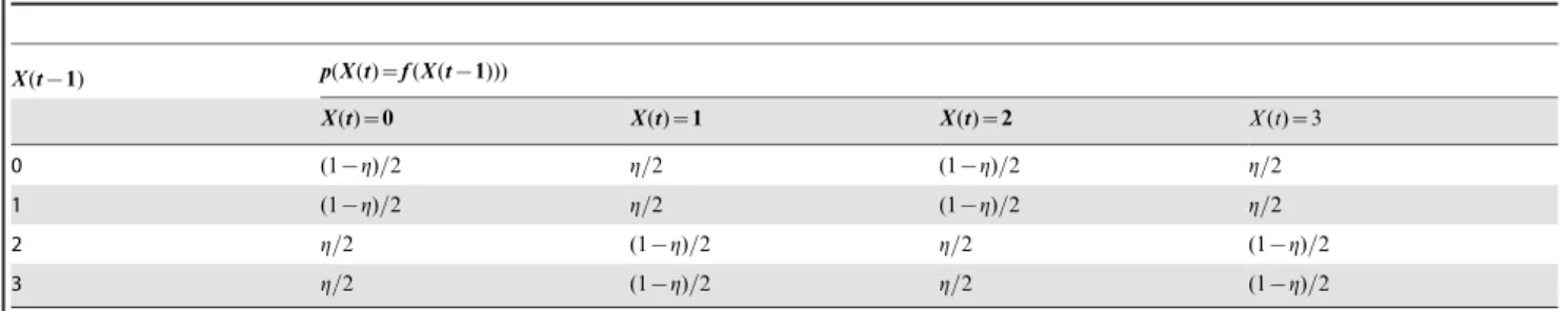
Figure 2. Causal graph for two coupled systemsX?Y.Illustration of d-separation ofXt{d{jandYtby(Xt{d,Yt{1). Arrows indicate a causal influence (directed interaction). Solid lines indicate a single time step, broken lines an arbitrary number of time steps. The black circle is the state to be predicted in Wiener’s sense, the red circles indicate the states that form its set of parents in the graphs. These states are also the ones conditioned upon in the novel estimatorTESPO. The blue circle indicates the state in the graph for which we want to determine that forms a Markov chain: Xt{d{j?(Xt{d,Yt{1)?Yt. Forj=0all sequential paths fromXt{d{jintoYtare blocked, as are the divergent paths between these nodes. All convergent paths (e.g. viaYt{din (B)) are not blocked. This holds forjw0(A) andjv0(B).
We also note that some constraints apply: (a) If the two systems cannot be directly observed, but only noisy observationsXX~,YY~ of the true systems dynamics are available, theorem 1 cannot be proven for these noisy observationsXX~,YY~, but may hold for many cases – see the examples given int the results section. We can also provide a proof (not given here) for autoregressive, linearly, unidirectionally coupled systems, where at most one of the two observations is noisy, i.e. we have X,YY~. However, counter examples can be found for very pathological structures of the noise on the two systems, that are not expected in physical systems (multi modal combinations of d-distributions). (b) Simulations show that for Gaussian noise of low amplitude, delays can still be identified correctly. (c) If the bidirectional coupling leads to full synchronization of the two systems, such that the probability distributions in equation 17 are delta distributions, transfer entropy is not defined. (d) There must be no other indirect sequential paths Xt{d{j?Zt{v?Yt (for some dzjwv§1) via some other variableZwhich are not blocked by(Xt{d,Yt{1)since this would violate the d-separation here. Extensions of the proof to this situation are conceivable, but are the topic of future studies.
Inability of Momentary Information Transfer to Reconstruct Coupling Delay
In order to contrast TESPO(Y?X,u) with the momentary information transfer (MIT) MIT(X?Y,u)~I(Yt;Xt{uD Yt{1,Xt{u{1) [36], we next examine two test cases. Case (Ia) contains noisy short-term source memory which leads to an erroneous delay estimation by MIT; in contrast, case (Ib) is an example that was reported to produce erroneous results inTESPO in [36], but we show here that this was due to the use of a symbolic preprocessing step in [36] and thatTESPOis perfectly capable to reconstruct the correct delay.
As explained in the methods section, in test case (Ia) Yt is a direct function ofXt{1, whileXt{1itself is a noisy mapping from
Xt{2 (with noise parameter g, also see table 1 ). As such,u~1 should be identified as the correct interaction delay here, although the source memory makes u~2 a potential candidate for an incorrect identification. The dynamics for test case (Ia) were run to provide 106 observations for estimating the required probability distribution functions. The estimation of the modified transfer entropy functional and the momentary information transfer was performed for this test case with the open-source ‘‘Java Informa-tion Dynamics Toolkit’’ [40] as detailed in the Methods secInforma-tion.
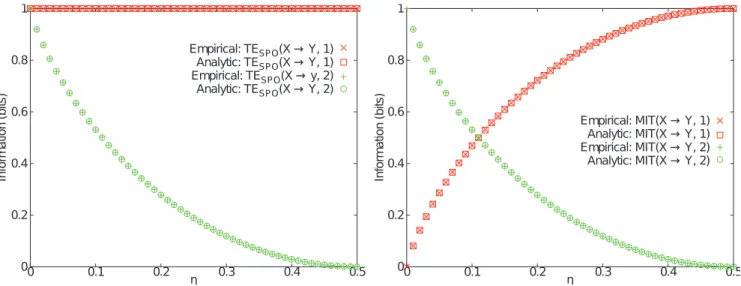
Figure 3 shows the results of measuringTESPO(Y?X,u)and MIT(X?Y,u), with delays u~1 and 2, as a function of the source noise parameter g. We see that, in line with our earlier proof regarding this situation of unidirectional coupling, TESPO(Y?X,u) consistently identifies the correct delay u~1, since TESPO(Y?X,u~1)wTESPO(Y?X,u~2) for all gw0. On the other hand, for a significant range ofg,MIT(X?Y,u)is
deceived by the source memory into incorrectly identifyingu~2
as the relevant delay.
CertainlyMIT(X?Y,u)fulfills its design in identifying the lag to the time step of the source where the relevant information in the target first appeared. As we see in this example however, the existence of some information regarding the target variable in the source at a certain lag does not mean that this relevant information was transferred to the target at that particular lag. Here, the memory in the source makes the source strongly correlated to the target over lagu~2. This drives both measures to high values for u~2 with low noise g, yet while TESPO(Y?X,u~1) remains higher still, MIT(X?Y,u~1) conditions out this correlated information and so falls belowMIT(X?Y,u~2). MIT returns the wrong result here because the conditioning on previous source state is not necessary and removes relevant information.
Finally, we examine test case (Ib), a bidirectionally coupled logistic map, for which Pompe and Runge [36] found that the TESPO(X?Y,u)incorrectly identified the interaction lag asu~1 instead ofu~2, when this quantity was estimated using symbolic mapping (capturing ordinal relationships). In contrast to the findings in [36], our analysis described in the methods section using Kraskov-Grassberger-Sto¨gbauer estimators [41] is able to accurately identify the correct lag u~2 as having larger TESPO(X?Y,u) (2.123 bits foru~2as compared to 0.826 bits for u~1). This result is in line with our proof that TESPO(X?Y,u) is maximized at the correct delay even in the case of bidirectional coupling. It is also in line with the more detailed empirical results we obtained for bidirectionally coupled processes as presented below. The opposite finding in [36] appears to simply be an artifact of their symbolic mapping approach: symbolic mapping may be a useful technique to handle small data sets, but it certainly removes parts of the information about the processes, and this information may well be relevant. Certainly, this is the case with coupled logistic maps, where examining ordinal relationships will miss many of the subtleties regarding how consecutive states are updated by the map.
Estimating Interaction Delays from Simulated Data
Here, we test the capability ofTESPOto detect the interaction delays from a series of simulated and experimental time series. The different cases cover stochastic, deterministic and real time series, representing different interaction configurations and delay ranges, and are described in detail in the methods section. The estimation of the modified transfer entropy functionals in these test cases (II-IX) was performed with the open-source MATLAB toolbox TRENTOOL [42] as detailed in the Methods section. State space reconstruction was performed using the Ragwitz criterion [39] in TRENTOOL, to obtain states that allow optimal self prediction, given the data. Throughout this section the estimated delays are
Table 1.Definition of stochastic self-mapping updatesf with memory and noise for variableXin test case (Ia).
X(t{1) p(X(t)~f(X(t{1))) X(t)~0 X(t)~1 X(t)~2 X(t)~3 0 (1{g)=2 g=2 (1{g)=2 g=2 1 (1{g)=2 g=2 (1{g)=2 g=2 2 g=2 (1{g)=2 g=2 (1{g)=2 3 g=2 (1{g)=2 g=2 (1{g)=2 doi:10.1371/journal.pone.0055809.t001
indicated by^dd, whereas the true, simulated delays are indicated by d.
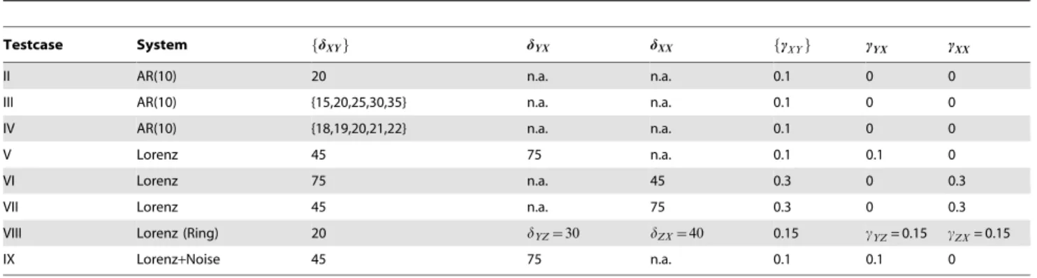
Overview of simulated test cases II-IX. Figure 4 presents the general structure of test cases (II-VII,IX). All these cases comprise two systems labeled as X,Y, which are either both autoregressive order 10 processes (AR(10), equation 29), or both Lorenz systems (Lorenz, equation 32). For the Lorenz systems, the second coordinate (V- see equation 32) was used as the observable producing the time series used for analysis. The systems may interact in the directionX?Y, with either a single delaydXY, or a set of delays fdXYg, with coupling strengths cXY or fcXYg, respectively. In the reverse directionY?Xwe only consider the case of single interactions with parameters dYX, and cYX. Additionally, in some of the cases delayed self feedback is present from processX to processX, with delaydXX, and strengthcXX. All simulated interactions, including self-feedback, were non-linear (quadratic) functions. One additional case (VIII) investigates delay reconstruction from a unidirectionally coupled ring structure of three Lorenz systems; the last case (IX) simulates the effects of observation noise on delay reconstruction. Details of the test cases are presented in table 2. For each test cases 50 data segments (trials) of 3000 sampling points each were simulated, resulting in a total of 150.000 data points. A full description of the generating equations for the system dynamics and the simulation details can be found in the subsection on the test cases in the methods section. In the following, we present results for these eight test cases (II-IX), with test case (V) serving as an example for the inability of the ‘old’ estimator [9,12,13,29] to recover the correct interaction delays.
Recovery of a single interaction delay. In test case (II) we investigated two unidirectionally coupled autoregressive (AR) processes where a single interaction delaydXY~20was present. We investigatedTESPO as a function of the assumed interaction delayu. Figure 5 shows the results of computingTESPO and its statistical significance (with a null hypothesis of no source-target coupling, see Methods) for the two possible directions of interaction,X?Y and Y?X. TEX?Y
SPO shows a maximal value foru~20units, which matches the nominal value of 20 sampling
steps.TEX?Y
SPO is statistically significant across a certain interval of delays around the maximum (14 to 23 sampling points) even when corrected for multiple comparisons. This blurring of the statistical significance of the predictive information transfer can be partly explained by memory in the source X (via autoregressive terms) meaning the predictive value of the actual directly influential scalar observation xtz1{d of the source is detectable in states xtz1{uofX bothbefore and afterthe actual delayu~d(compare the extension of sources states indicated by shaded boxes in figure 1). An additional factor here is that examination of the source statesxt{u(instead of scalar observationsxt{u) means that full information about the directly influential observationxtz1{dis contained in several source states after xtz1{d. Crucially, the opposite direction (Y?X) reveals a flat profile with no statistical significance, in correspondence with the absence of a directed interaction from processYtoX.
Recovery of multiple interaction delays. In the test case (III), we investigated two unidirectionally coupled AR processes where multiple interaction delays dXY were present,
Figure 3. Test case (Ia), comparison of MIT and TE.Analytic and empirical measurements of (a) Transfer entropyTESPO(X?Y,u)and (b) Momentary information transferMIT(X?Y,u)as a function of memory noise parametergfor the discrete-valued process with short-term source memory and a delayd~1. Each measure is plotted for delaysu~1(red) and 2 (green). The correct causal interaction delay coorspondsu~1and therefore we expect an appropriate measure to always return a higher value withu~1than withu~2, i.e the red curve should always be at higher values than the green curve. Nevertheless, there is potential foru~2to be identified erroneously as the delay due to the presence of memory in the sourceX, and MIT indeed finds this result for a range of the memory noise parameterg(below~00.1).
doi:10.1371/journal.pone.0055809.g003
Figure 4. Overview over the structure of simulated test cases II-IX.Note that not all combination of links and parameters are always investigated. For details refer to table 2.
dXY~15,20,25,30,35. Figure 6 reveals that they can be readily detected by scanning TESPO. Well separated peaks indicate the presence of multiple delays around values of,14, 19, 25, and 30 sampling units for the direction of interactionX toY. The curve displays an additional shoulder at u~35. Nominal delays in the simulations were 15, 20, 25, 30 and 35, and thus all but the longest delay were correctly detected. The longest delay is most likely not detected because much information from the relevant source state xtz1{dhas already been communicated to the target over several shorter delays, due to the inherent memory of the AR(10) process, and there is no longer enough novel information provided by the source given the past state of the target to evoke a clear peak. However, the transfer entropy values TESPOX?Y indeed were
statistically significant up to an assumed delay of 35 units, in line with the maximal delay simulated.
A more complex case (IV) is encountered when dealing with a smooth distribution of delays. Figure 7 demonstrates that in this case, a peak of TESPO is attained near to the mean of the distribution of delays. The width of the peak is proportional to the width of the delay distribution. However, an exact estimation of the range of delays is difficult since single delays are also associated with broad peaks in theTESPOversus assumed delay curves (see figure 5, but note the different scale of the time axes). We note that the peak of TESPO is skewed towards the shorter of the actual interaction delays, and this may be due to: (a) the longer delays providing less novel information from the source given that it is already contained in the target state from the shorter delays (as discussed in the above paragraph); and/or (b) the persistence of information of the current influential componentxtz1{d of the source statextz1{din several following source states (as discussed in the preceding subsection).
Recovery of delays of bidirectional interactions. For the analysis of two bidirectionally coupled Lorenz systems in test case (V), withdXY~45anddXY~75, transfer entropy values peaked at u~46andu~76samples for the interaction from processXtoY,
Table 2.Parameter settings used to create the simulated test cases II-IX.
Testcase System fdXYg dYX dXX fªXYg ªYX ªXX
II AR(10) 20 n.a. n.a. 0.1 0 0
III AR(10) {15,20,25,30,35} n.a. n.a. 0.1 0 0
IV AR(10) {18,19,20,21,22} n.a. n.a. 0.1 0 0
V Lorenz 45 75 n.a. 0.1 0.1 0
VI Lorenz 75 n.a. 45 0.3 0 0.3
VII Lorenz 45 n.a. 75 0.3 0 0.3
VIII Lorenz (Ring) 20 dYZ~30 dZX~40 0.15 cYZ= 0.15 cZX= 0.15
IX Lorenz+Noise 45 75 n.a. 0.1 0.1 0
Lorenz = chaotic Lorenz system; AR = autoregressive processes. For the meaning of the coupling and delays constantsfd::gandc::refer to figure 4. doi:10.1371/journal.pone.0055809.t002
Figure 5. Test case (II). Transfer entropy (TESPO) values and significance as a function of the assumed delayufor two unidirection-ally coupled autoregressive systems. For visualization purposes all values were normalized by the maximal value of the TE between the two systems, i.e. max (TEX?Y
SPO (u),TEYSPO?X(u)). Red and blue color indicate normalized transfer entropy values and significances for interactions X?Y and Y?X, respectively. The nominal interaction delaydXY used for the generation of the data was 20 sampling units from the processXtoY. Asterisks indicate those values ofufor which the p-valuev0.05 once corrected for multiple comparisons. Missing
points forTEY?X
SPO (u))are because the analyses for theseu’s failed to pass the shift test (a conservative test in TRENTOOL to detect potential instantaneous cross-talk or shared noise between the two time series, see [42]).
doi:10.1371/journal.pone.0055809.g005
Figure 6. Test case (III). Transfer entropy (TESPO) values and significance as a function of the assumed delayufor two unidirection-ally coupled autoregressive systems with multiple delays. The simulated delaysfdXYgwere 15, 20, 25, 30 and 35 sampling points. The rest of the parameters and criteria used are the same as those in Figure 5. doi:10.1371/journal.pone.0055809.g006
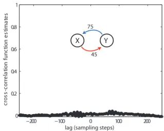
andYtoX, respectively (Figure 8). These values differed only by one sample from to the true interaction delays used for simulation. Moreover, the relation between the transfer entropy values for the two coupling directions reversed with increasing delay parameter u: for delay values up to 65, transfer entropy values were larger for the direction from processX toY, for values ofularger than 65 the opposite was the case. This is an important finding as the difference of the transfer entropies in both directions, also called the net transfer entropy, is often used as an indicator of the effective or dominating interaction structure. However, in our example, this net information transfer changed sign with changing delay parameteru. As an additional result, we show that the cross correlation function between the signals of the two systems was flat (Figure 9), as expected for a quadratic coupling.
Failure of the traditional estimator to recover the correct delays. We also analyzed the case (V) of bidirectionally coupled Lorenz systems with the ‘old’ estimator (u0~u) from references [9,12,13,29] (figure 10). As expected on theoretical grounds, this type of estimator did not recover the simulated delays for the two coupling directions (dXY~45anddYX~75), but instead delivered erroneous estimates (^ddXY~28and^ddYX~61).
Recovery of the delay of a feedback loop. We consider here the cases (VI) and (VII) where a feedback loop is affecting the dynamics of a node. In particular, we investigate first how the presence of feedback can be detected, and second how a feedback loop in a node affects estimation of transfer entropy to a different node.
We note that feedback loops do not pose a principal conceptual problem. Mathematically, a perfect state space reconstruction (see Methods for an explanation of state space reconstruction.) would subsume the feedback activity into the node’s dynamics. In practical terms, however,longself-feedback delays – in comparison to the intrinsic dynamics of the node – can not be covered practically in Taken’s classical state space reconstruction [43]. The reasons for this are twofold: (1) Self prediction performance may become unstable in high dimensional state spaces necessary to recover the delayed self-feedback. Algorithms determining optimal embedding parameters by optimal self prediction may get stuck in local minima this way. (2) Computational cost quickly diverges
with a growing number of dimensions in state space. Hence, one may not even include the necessary number of dimensions and the necessary range of embedding delays in the parameter ranges that are searched to get the optimal embedding values. Given an imperfect state space reconstruction, even our new estimator is no longer self-prediction optimal, then. In the following we show that this estimator is nevertheless useful to detect self-feedback under conditions of long self-feedback delays.
Thus, we start by considering the dynamics of a single Lorenz system (processX in test case (VI)) subject to a non-linear delayed feedback loop. This is, its own past output is fed back after it has undergone a nonlinear (quadratic) transformation (see the section ‘test cases’ in Methods). To detect the presence of feedback activity we evaluateTESPO(X?X,u) between the system’s original time series and its own pastutime steps back. To this end we choose embedding parameters such that the reconstructed states do not
Figure 7. Test case (IV). Transfer entropy (TESPO) values and significance as a function of the assumed delayufor two unidirection-ally coupled autoregressive systems with multiple delays. The simulated delaysfdXYgwere 18, 19, 20, 21 and 22 sampling points. The rest of the parameters and criteria used are the same as those in Figure 5. doi:10.1371/journal.pone.0055809.g007
Figure 8. Test case (V). Transfer entropy (TESPO) values and significance as a function of the assumed delayufor two bidirectionally coupled, chaotic Lorenz systems. The simulated delays weredXY~45 anddYX~75, and the coupling constants werecXY~cYX~0:1. The delays were recovered as^ddXY~46and^ddYX~76. For more parameters see table 2.
doi:10.1371/journal.pone.0055809.g008
Figure 9. Test case (V). Crosscorrelation function for the two quadratically coupled chaotic Lorenz systems from figure 8.
cover the feedback delay. The results are shown in Figure 11. Clear peaks are observed at u~45, which corresponds to the simulated feedback delay dXX, and its integer multiples. This corresponds to information being fed back via multiple rounds of the feedback loop.
The presence of feedback loops can challenge the reliable detection of information transfer between nodes. For example, if a node subject to feedback is unidirectionally coupled to another node, the direct computation of transfer entropy between the two nodes as a function of a delay parameter can lead to wrong inferences. To illustrate this point, we computed the self prediction optimized transfer entropy between the Lorenz system (X) with a feedback loop and another Lorenz (Y) which receives its output.
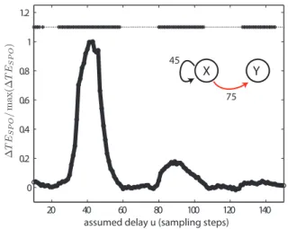
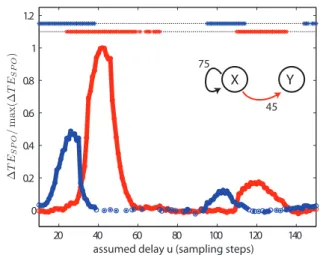
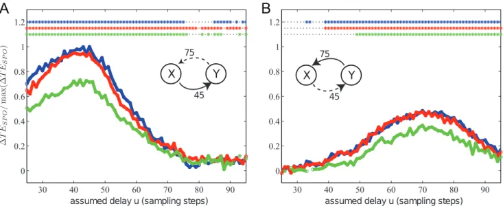
First, we consider test case (VI) in which the feedback loop time (dXX~45) is shorter than the interaction delay between the systems (dXY~75). As shown in Figure 12,TESPOX?Yhas the highest peak at u~75, corresponding to the simulated interaction delay. However, it also shows clear peaks atu~30andu~120, values which amount to the difference between the interaction and feedback delays, and their sum respectively. In general, peaks were observed at u~dXYzndXXw0;n[Z, corresponding to different combinations of cycles around the feedback loop plus the interaction delay.
TESPO fromY toX, the direction in which no coupling was simulated, also exhibits several weak but significant peaks, i.e. we find false positive results in this case. Peaks were present at multiples of the delay feedback time minus the propagation time between the two Lorenz systems (u~ndXX{dXYw0;n[Z). These peaks inTESPOfromYtoXappear because the feedback loop in processX results in recurrent information in the dynamics of X that can be predicted by the processY, because thew processY also receives a copy of them via the connection X?Y. This information is useful to predict the state ofX when the assumed delayuinTESPOfromYtoXis at least as big asu~ndXX{dXY, withnchosen such thatuis positive. Notice that the size of the peaks decreases with largern.
Second, we considered test case (VII) in which the feedback delay dXX is longer than the interaction delay time dXY (see
Figures 13 and 14). In this case structure similar to test case (VI) is observed for the location of the peaks of TESPO. However, TEY?X
SPO shows higher and more false positive peaks than in case (VI). This occurs since whendXXwdXY, processYcan predict the
Figure 10. Test case (V) analyzed with the old estimator.
Transfer entropy (TE) values and significance estimated by the old estimator from references [9,12,13,29] as a function of the assumed delayufor two bidirectionally coupled, chaotic Lorenz systems. The simulated delays were dXY~45 and dYX~75. These delays were recovered erroneously as^ddXY~28and^ddYX~61. For more parameters see table 2.
doi:10.1371/journal.pone.0055809.g010
Figure 11. Test case (VI) - self-feedback analysis.Transfer entropy (TESPO) values between past and present of one of two Lorenz systems (X) and significances as a function of the assumed delay u. The analyzed chaotic Lorenz system was subject to a feedback loop with delaydXX~45, and an outgoing interactionX?Ywith delaydXY~75, but no incoming interaction. The recovered delay for the self feedback was^ddXX~43, with a sidepeak at around two times this value. For the interaction analysis X?Y see figure 12. For more parameters see table 2.
doi:10.1371/journal.pone.0055809.g011
Figure 12. Test case (VI). Transfer entropy (TESPO) values and significance as a function of the assumed delayufor a unidirectionally coupled chaotic Lorenz systems. The first Lorenz is subject to a feedback loop (dXX~45) and unidirectionally couples to a second Lorenz with a interaction delay ofdXY~75samples. Recovered delays were^ddXX~43(see figure 11), and^ddXY~73. Sidepeaks were observed for^ddXY close todXY+n:dXX. Spurious interactions were observed in the reversed direction at^ddYX~n:dXX{dXY, as it is expect for a system with self feedback [45]. Considering the positive test for self-feeback (figure 11) and the recovery of the self-feedback delay, the true system connectivity can be derived by combining the analysis of self-feedback and interaction delays.
transitions that will occur inX already after a single delay loop, because even for n~1 the condition u~ndXX{dXYw0 is fulfilled, – in contrast to a prediction of two delay loops ahead as in the previous case above. This situation is related to the so-called anticipative synchronization in which a slave system (Y) can anticipate the dynamics of the master system when this is subject to a long feedback loop [44,45].
To be clear: these observations are not a theoretical problem withTEY?X
SPO but are a practical issue in estimation (due to the impracticality of adequately forming Taken’s embedding ofX in the presence of the long delay loop, as described above).
Ring of Lorenz systems. In a network of three Lorenz systems coupled into a unidirectional ring, test case (VIII), our method identified the three simulated delaysdXY~20,dYZ~30, dZY~40 with reasonable precision as ^ddXY~21, ^ddYZ~28,
^
d
dZX~38(figure 15). Analysis of self-feedback (as it is in principle present in a ring structure) for systemX resulted in no significant peak at the expected sum of all three simulated delays (90), indicating that the information originally transfered from system 1 into the ring iseffectivelywiped out by the chaotic dynamics of the next nodes in the ring, a phenomenon well known in from coupled chaotic laser systems [46].
Effects of observation noise. In test case (IX) we simulated two bidirectionally, quadratically coupled Lorenz systems with delays dXY~45, dYX~75, and added independent, Gaussian, white noise to the time series of theV-coordinate (see equations 32, 33 for details) before the reconstruction of delays. Observation noise did degrade the precision of delay reconstruction to a certain degree: with 1%, 2% and 9% of the total signal variance contributed by noise, the estimated delays were^ddXY~45,40,42, and ^ddYX~70,72,70 (figure 16). Note that noise amplitude and delay reconstruction error do not seem to be systematically related, suggesting that the effects of particular realizations of finite data cause the reconstruction errors.
Local Field Potential Data
To demonstrate that interaction delays can be reconstructed from biological time series with sufficient precision, we analyzed recordings of the electroretinogram (R) and local field potentials from the tectum (T) of the turtle brain (Pseudemys scripta elegans, figure 17). These data were recorded during stimulation (S) with light flashes at time points determined by a random process and with a duration drawn from a uniform random distribution; this ensured stationarity of the time series. In this experiment, direct physical interactions existed from the light source to the retina and from the retina to the tectum (S?R?T). In addition, there was an indirect interaction from the light source to the tectum, mediated by the retina. This opens the possibility to check the precision of the delay reconstruction despite the fact the we have no precise knowledge of the true biological interaction delays. The evaluation of reconstruction precision is possible because the interaction delays reconstructed from S?R and from R?T should sum up to the interaction delay reconstructed fromS?Tif reconstruction is precise.
We reconstructed the interaction delays the same way as in all previous test cases by scanningu. Indeed, the reconstructed delays were: ^dd(S,R)~30ms, ^dd(R,T)~12ms, ^dd(S,T)~44ms, meaning that the reconstructed delays between light source and retina and between retina and tectum added up to the reconstructed delay between light source and tectum with an error of 2 ms or 4.5%. Discussion
Transfer Entropy Estimation without Violating Wiener’s Principle
We have laid out in the introduction why the earlier formulation of transfer entropy with an explicit time-delay as given in equation 3 and as used in [9,12,13,29] is not a precise formulation of
Figure 13. Test case (VII) - self-feedback analysis. Transfer entropy (TESPO) values between past and present of one of two Lorenz systems (X) and their significances as a function of the assumed delayu
for a single chaotic Lorenz system subject to a feedback loop with delay dXX~75, and an outgoing interactionX?Ywith delaydXY~45. The recovered delay for the self feedback was^ddXX~74, with a sidepeak at two times this value. For the interaction analysisX?Y see figure 14. For more parameters see table 2.
doi:10.1371/journal.pone.0055809.g013
Figure 14. Test case (VII). Transfer entropy (TESPO) values and significance as a function of the assumed delayufor a unidirectionally coupled chaotic Lorenz systems. The first Lorenz is subject to a feedback loop (dXX~75) and unidirectionally couples to a second Lorenz with a interaction delay ofdXY~45samples. Recovered delays were^ddXX~74(see figure 13), and^ddXY~44. Sidepeaks were observed for^ddXY close todXY+n:dXX. Spurious interactions were observed in the reversed direction at^ddYX~n:dXX{dXY, as it is expect for a system with self feedback [45]. Considering the positive test for self-feeback (figure 13) and the recovery of the self-feedback delay, the true system connectivity can be derived by combining the analysis of self-feedback and interaction delays.
Wiener’s principle of causality in information-theoretic terms, as it violates the requirement of optimal self-prediction of the target time series. Accordingly, we were able to construct a test case were this functional gives a wrong estimate of the interaction delay in a system (figure 10), while the novel functional proposed here (equation 7), gives the correct result (figure 8). We therefore suggest to use this novel functional wherever interaction delays are expected. Accordingly, the new functional has been implemented in version 2.0 of our open source toolbox for transfer entropy estimation, TRENTOOL [42], and has been made the default option.
Interaction Delay Reconstruction by Maximizing Predictive Information Transfer
In this study we demonstrated that it is possible to reconstruct the delays of interactions between two systems by finding the maximum of the predictive information transfer estimated by a novel transfer entropy functional, TESPO, with a parametric dependence on the interaction delay. Our work complements
earlier, anecdotal reports of delay-sensitivity of the predictive information transfer [12,13,42], by presenting a new formulation of the transfer entropy functional rigorously based on Wiener’s principle of causality andbacked by a formal proof(see results section). Crucially, our experimental results identify the precise interaction delay for coupled systems with a single interaction delay, validating the formal proof which was constructed under these conditions. Furthermore though, we show that the reconstruction of interaction delays is possible for a large range of coupling types, multiple interaction delays, complex dynamics of the subsystems, for ring, and bidirectionally coupled systems. This last point is of great importance, as up to now, the analysis of bidirectionally coupled systems has often been discouraged, at least implicitly. Hesitation to analyze bidirectionally coupled systems is based on two observations - on the one hand, bidirectional coupling often leads to complete synchronization and in these cases an analysis of interactions is indeed not possible - on the other hand, it has been shown that the quantification of causal effect size is not always possible in these systems [47]. With our finding that in cases where
Figure 15. Test case VIII.Transfer entropy (TESPO) values and significance as a function of the assumed delayufor three unidirectionally coupled chaotic Lorenz systems. The First Lorenz couples with the second Lorenz with an interaction delay ofdXY~20samples, the second Lorenz is unidirectionally coupled with the third Lorenz at a delay ofdYZ~30samples and the third Lorenz is unidirectionally coupled with the first Lorenz at an interaction delay ofdZX~40samples. The reconstruction of the simulated delays were: (A) self feedback,^ddXX~2, this value may be due to insufficient embedding, (B)^ddXY~21, (C)^ddYZ~28, and (D)^ddZX~38.
there is no complete synchronization we can reconstruct at least the individual delays of bidirectional coupling (again backed by our formal proof), we hope to revive the analysis of such systems -that are abundant in nature and technology.
Formally identical functionals to TESPO have been indepen-dently introduced several times in the literature, first by Nichols and colleagues [48], then by Overbey and Todd [49] – both in the field of structural integrity analysis of mechanical systems. In addition, Ito and colleagues used a formally identical functional to increase the detectability of interactions in spiking neural data [50]. In none of these studies the use of the functional for explicit delay reconstruction has been recognized and as a consequence no proofs for this property have been given. Ito and colleagues did indeed state that the delay parameter in their equation is there to account for finite delays, but they simply assumed maximality of the functional at the correct delay, without proof.
Note that the successful reconstruction of the true interaction delay between two coupled systems depends on reliable and precise enough estimates of the corresponding information-theoretic quantities (see methods section for the algorithms applied here). Obtaining these estimates may become a problem for small sample sizes. In this case, additional statistical testing against the null hypothesis of no coupling should be included when scanning delays and only maxima that show statistically significant coupling should be evaluated.
In addition, stationarity of the time series entering the analysis must be given, because transfer entropy between two random processes is typically defined via a time average that can only be used instead of the proper ensemble average for random processes if stationarity is given. If stationarity cannot be assumeda priorifor the time series under investigation, appropriate testing should be performed (see [51,52] and references therein). If at least cyclostationarity can be guaranteed, the proposed method could be used as functional within the ensemble averaging framework described in [53]. Reliably repeated non-stationarities may also be removed using the mathematical methods presented in [54]. In this case, however, additional testing for remaining non-stationa-rities is recommended. Note that for the local field potential data
Figure 16. Test case IX.Transfer entropy (TESPO) values and significance as a function of the assumed delayufor two bidirectionally coupled, chaotic Lorenz systems. The simulated delays weredXY~45anddYX~75. Observation noise with different amplitude was added to the simulated time series of the processes. The delays were recovered as (A)^ddXY~45anddd^YX~70for S=N~45:88db(blue), ^ddXY~40and (B) ^ddYX~72for S=N~37:74db(red) and^ddXY~42andd^dYX~70forS=N~23:84db(green).
doi:10.1371/journal.pone.0055809.g016
Figure 17. Interaction delay reconstruction in the turtle brain.
(A) Electroretinogram (green), and LFP recordings (blue), light pulses are marked by yellow boxes. (B) Schematic depiction of stimulation and recording, including the investigated interactions and the identified delays.
analyzed here, approximate stationarity was guaranteed by stimulation at multiple randomly chosen time points within each epoch of the experiment time series (i.e. ‘‘trial’’), with stimulation durations also drawn from a random distribution.
Comparison to the Momentary Information Transfer
As detailed in the methods section,momentary information transfer (MIT) [36] is an alternate approach to reconstructing the interaction delay, again using a scanning approach to maximize MIT as a function of delayu. BothTESPOand MIT condition on the immediately previous target state (which is correct in comparison to the old TE estimator), and given thatTESPO uses an embedded source stateXt{u, both measures includesynergistic information that is jointly contributed by fXt{u,Xt{u{1g (as opposed to TE computed using only a single sourceobservation). Yet a stark difference is the extra conditioning by MIT on Xt{u{1, which removesredundantinformation that was already contained in the source. This prevents any of this information from being attributed to transfer at the lagu.
A major conceptual difference between the Pompe and Runge study and ours is that no formal proof of the maximality of their functional MIT at the correct interaction delay is given, and as we argue below cannot be given.
Indeed, we provide a counter-example here – in test case (Ia) – where the momentary information transfer is not necessarily maximized at the correct interaction delay, in direct contrast to our proof of this property forTESPO. As such, MIT is not always reliably inferring the correct interaction delay.
The intention of the MIT in removing the self-redundant information in the source was to find the delay at which the relevant information about the target’s state update first appeared in the source. However, the availability of such information in the source at a specific time point does not mean that it is being transferred at that instant, and the presence ofmemoryin the source inevitably leads the MIT to underestimate the influence of the source at the actual interaction delay (because of the removal of redundant, though potentially transferred, information). We dem-onstrated for these reasons that the MIT failed to identify the correct interaction delay in test case (Ia) on a simple, unidirectional coupling, single-interaction delay example with source memory, whereas ourTESPO estimator functioned correctly.
As argued in [55], when investigating effective connectivity, the removal of redundant information by prematurely conditioning on other potential sources reduces our ability to infer connections. Conditioning on the source at another delay(s) should only be performed once one has already established the primary (or additional) coupling delay (see further discussion below and in [34,55]).
Furthermore, the actual MIT analysis in [36] was carried out on a symbolic mapping of the time series (to vectors capturing the ordinal relationships between the variables). This approach, while potentially useful for short time-series realizations in magnifying certain relationships in the data, removes information on absolute values of the variables involved. While this loss of information may be harmless in climatology – the field of research MIT was aimed at –, it might be crucial to retain this information in other fields, such as neuroscience. Indeed, for the example in their study ([36], Section V.A) where theTESPO was not able to infer the correct interaction delay but MIT was, we have shown in test case (Ib) that this result is an artifact of the symbolic mapping in [36] rather than the measures themselves. Specifically, when we estimated in the continuous domain (retaining much information that the symbolic mapping removed), TESPO correctly identifies the interaction lag in this coupled logistic map process.
Interaction Delay Fingerprints in Systems with Self-feedback
The phenomenon of self feedback is present in many complex networks. This self feedback can arise genuinely in the nodes of the network, e.g. by mechanisms such as autapses in neural networks [56], or because the systems receives (transformed) self-feedback via an unobserved part of the network. The analysis of interaction delays via TESPO may offer valuable hints with respect to the presence of absence of relevant self-feedback.
Here we showed that TESPO can detect the presence of feedback loops when applied to the time series of a single system and its own past – even if the system is chaotic and the feedback loops entail nonlinear transformations of the systems output. The information on the delay of a feedback loop can then be used to disentangle the potentially complex delay fingerprints, consisting of multiple peaks, that arise if such a system with self-feedback is coupled to other systems.
In principle, the multiple spurious peaks in the directionX?Y in our example, and all of the peaks in the directionY?Xshould vanish, given a state space reconstruction with states long enough to cover the delay feedback time. However, very long reconstruc-tion lengths might lead to instable estimates due to the ‘curse of dimensionality’ [57]. In such a case, where the practically feasible reconstruction lengths for states are too short to cover the full dynamics of a system, the identification of feedback loops by TESPOhelps to better interpret the estimated pairwise information transfers between the nodes of a network. Time points around the self-feedback delay could in addition be included into the embedding states of anon-uniform, data-efficient embedding scheme [34], which would assist in removal of information storage and more accurate assessment of the transfer entropy as per the principles outlined in subsection on Wiener’s principle above.
TESPO differs from a simple application of the lagged auto-mutual information functional (AMIF) in that active information storageI(Xt;Xt{1)[37] contained in the most recent reconstruct-ed state Xt{1 is removed. This will accentuate the presence of peaks in the delay spectrum compared to AMIF.
Information Transfer Delays from Noisy Time Series
The proof for the identifiability of the true delay in the information transfer between two time series holds strictly only for the case of zero observation noise. Indeed the fundamental differences between time series obtained from Markov systems and those obtained from hidden Markov systems (i.e. from noisy observations) make it difficult to extend our proof without specifying the noise explicitly in each case. Nevertheless, our simulations of typical noise influences – such as independent, Gaussian, white noise – show that our approach works well in practice. While noise does indeed degrade precision, the random relation between observation noise amplitude and delay recon-struction error suggest that these errors are due to the combined effects of finite data and noise, and can be alleviated by increasing sample size.
Relation to Linear Granger Causality and Corresponding Time Delay Reconstruction Procedures
Recently, Barnett and colleagues [19] demonstrated that transfer entropy and linear Granger causality are equivalent for the case of data with a Gaussian distribution. This result greatly simplifies the computation of interactions for data of this class. Neural data, however, do most likely not have a Gaussian distribution. This can for example be seen when comparing brain electrical source signals from physical inverse methods with the
time course of corresponding ICA components [58]. Given that ICA components are as non-Gaussian as possible by definition, and given the fact that ICA components and brain source signals extracted by inverse methods closely match, we can interpret this as evidence for a non-Gaussian nature of brain signals. For these signals, TE may have an advantage for the analysis of directed interactions. On the other hand, the methodology presented here should be transferable to the domain of linear Granger causality in Gaussian data by virtue of the proof by Barrett and colleagues. Hence, the approach presented here may be seen as an alternative to earlier attempts to infer timing delays via linear Granger causality by inspecting time-dependent model-coefficients and using large model orders of 200 and more. For Gaussian data the scanning approach presented here would be equivalent to setting the firstn model coefficients to zero without having to estimate them, and scanning n, estimating thek next model coefficients, wherekis the embedding dimension, resulting from optimization via the Ragwitz criterion [39].
Relation of Delay Reconstruction and Multivariate TE Analyses
In systems composed of more than two interacting subsystems a pairwise, bivariate transfer entropy analysis as given by equation 7 may lead to wrong inferences with respect to the presence of an interaction between two subsystems. This happens when either a third subsystem drives the two subsystems under investigation with differential delays (‘common drive’), or when the two subsystems under investigation are connected indirectly via a third system acting as a relay (‘cascade effect’). The potential presence of interaction configurations of this kind can be detected by looking at timing relations across the graph of bivariate interactions. Here, this was demonstrated by our reconstruction of delays in LFP data in the turtle, where the interaction delay between light source and tectum was equal to the sum of delays on a route connecting the same end points (light source to tectum, via the retina). While both a common drive (light source?retina, light source?tectum) or cascade scenario (light source?retina ?tectum) could explain the manifestations of these delays, what is important here is that this result is consistent with the known biological indirect interaction via the retina. If the concern is just to avoid false positive detection of interactions, a simple delay analysis approach may be a data efficient alternative to fully multivariate treatments of TE [7,34,35,55]. That said, such multivariate treatments could yield further insights, e.g. if the conditional TE [7,35] from the retina to the tectum conditioned on the light source (with appropriate delays incorporated) were statistically non-zero, then this would eliminate the possibility that the inferred retina ?
tectum relationship was a result of common drive by the light source. Combining delay analysis with multivariate treatments is feasible but more complicated (delays must be determined in an appropriate order, in the same way that the self-conditioning delay u0was determined here before the source delayuwas explored -see some relevant discussion in [34,55]); and will be the subject of a future publication.
Delay Estimation Versus Significance Testing
We would like to stress here that inference on the presence of information transfer is a task separate from reconstructing the delay of the information transfer. For the former task we employed nonparametric permutation testing of TESPO against surrogate data obtained from exchanging data epochs in the source. For the latter we searched the peak of TESPO. Our simulation results demonstrate that the existence of information transfer can typically be assessed over a wide range of assumed delays. On
the one hand, this fact underlines the robustness of theTE SPO-functional against misspecification of the delay parameter. On the other hand it is a warning not to conclude from the presence of significant information transfer at a certain delay parameter that the true delay is close to the assumed delay, if no scanning of the delay parameter was performed.
A Practical Note on the Combination of Delay Reconstruction and Shift Testing
In practical applications, linear mixing or instantaneous cross-talk between signals occurs and may bias interaction measures based on Wiener’s principle [12,59]. To detect such crosstalk, we have proposed a so-called shift-test [12,13,42]. This test deter-mines if shifting the source time series into the past by the time that represents the assumed delay, u, increases TE. This way two predictive information transfer terms get compared: on the one hand the predictive information transfer from the past of the source to the target, on the other hand the instantaneous information transfer from source to target. This procedure works very well as demonstrated in [42], but gives rise to minor a technical problem for real world data, because in these data instantaneous cross-talk is never truly zero. For assumed delaysu that are much larger than the true delay, the information transfer will be arbitrarily small, due to the combined effects of conditioning on the past of the target and the finite memory of the source. In contrast, cross-talk will always be non-zero. Hence, in situations with some finite cross-talk, there will a largest delay parameter umax, beyond which the presence of crosstalk will always be reported by the shift test. This, however, can be easily seen by comparing TE values at largeuto those at smalleru. In contrast to a mere nuisance effect, relevant cross-talk should outweighTESPOeven at the optimal delay.
Conclusion
We present a novel transfer entropy functional, which is a rigorous formulation of Wiener’s principle of causality in information-theoretic terms, respecting the condition of optimal self-prediction of the target time series from its own past. This functional has an explicit parametric representation of interaction delays between interacting systems. Scanning this parameter in search of the maximal predictive information transfer allows one to reconstruct interaction delays from a wide variety of systems. Methods
Ethics Statement
Local field potential data were taken from experiments published elsewhere [42]. These animal experiments were approved by the German local authorities (Regierungspraesidium, Hessen, Darmstadt).
Practical Transfer Entropy Estimation
In this section we outline the particular estimator of the TESPO functional as provided in our toolbox TRENTOOL [42], and used in all analysis in this study. This realization relies on three steps: (1) state space reconstruction from scalar time series, (2) reformulation of the conditional mutual information in terms of four Shannon entropies, and (3) subsequent entropy estimation by a modified Kraskov-Stoegbauer-Grassberger estimator [41,42].
As causality and interactions are defined as properties of systems, not scalar time series, we first have to reconstruct the corresponding state space of the interacting systems from the scalar time series. For this purpose we used Takens delay