Copyright belongs to the author. Short sections of the text, not exceeding three paragraphs, can be used provided proper acknowledgement is given.
The Rimini Centre for Economic Analysis (RCEA) was established in March 2007. RCEA is a private, nonprofit organization dedicated to independent research in Applied and Theoretical Economics and related fields. RCEA organizes seminars and workshops, sponsors a general interest journal The Review of Economic Analysis, and organizes a biennial conference: The Rimini Conference in Economics and Finance (RCEF). Scientific work contributed by the RCEA Scholars is published in the RCEA Working Papers and Professional Report series.
The views expressed in this paper are those of the authors. No responsibility for them should be attributed to The Rimini Centre for Economic Analysis.
The Rimini Centre for Economic Analysis
75 University Ave W., LH3079, Waterloo, Ontario, Canada, N2L3C5 www.rcfea.org
WP 17-31
Dimitrios Bakas
Nottingham Trent University, UK
The Rimini Centre for Economic Analysis
Athanasios Triantafyllou
University of Essex, UK
T
HE
I
MPACT OF
U
NCERTAINTY
S
HOCKS ON
The Impact of Uncertainty Shocks on the
Volatility of Commodity Prices
Dimitrios Bakas
a,cand
Athanasios Triantafyllou
b†aNottingham Business School, Nottingham Trent University, UK bEssex Business School, University of Essex, UK cRimini Centre for Economic Analysis (RCEA), Canada
Abstract
In this paper, we empirically examine the impact of uncertainty shocks on the volatility of commodity prices. Using alternative measures of economic uncertainty for the U.S. we estimate their effects on commodity price volatility by employing both VAR and OLS regression models. We find that the unobservable economic uncertainty measures of Jurado et al. (2015) have a significant and long-lasting positive impact on the volatility of commodity prices. Our results indicate that a positive shock in both macroeconomic and financial uncertainty leads to a persistent increase in the volatility of the broad commodity market index and of the individual commodity prices, with the macroeconomic effect being more significant. The impact is stronger in energy commodities compared to the agricultural and metals markets. In addition, our findings show that the measure of unpredictability of the macroeconomic environment has the most significant impact on the commodity price volatility when compared to the observable measures of economic uncertainty that have a rather small and transitory effect. Finally, we show that uncertainty in the macroeconomy is significantly reduced after the occurrence of large commodity market volatility episodes.
Keywords: Economic Uncertainty, Commodity Prices, Volatility
JEL Classification:C22, E32, G13, O13, Q02
† Dimitrios Bakas: Nottingham Business School, Nottingham Trent University, Burton Street, Nottingham, NG1 4BU, United Kingdom, E-mail: [email protected].
Athanasios Triantafyllou: Essex Business School, University of Essex, Wivenhoe Park, Colchester, CO4 3SQ, United Kingdom. E-mail: [email protected].
1
1. Introduction
Uncertainty shocks have a significant negative impact on the macroeconomy (Bloom,
2009; Colombo, 2013; Jurado et al., 2015; Baker et al., 2016; Caldara et al., 2016;
Henzel and Rengel, 2017; Meinen and Roehe, 2017). According to these empirical studies, a rise in economic uncertainty (as measured by several alternative proxies proposed in the literature) has a negative effect on aggregate investment, industrial production and the employment rate. Moreover, many recent empirical studies indicate that Economic Policy Uncertainty (EPU henceforth) shocks, in the form
suggested by Baker et al. (2016), result to an increase in stock-market turbulence.1
While many studies verify this negative impact of uncertainty shocks on the macroeconomy and on the equity markets, there is only limited empirical evidence in the literature about the impact of uncertainty shocks on the volatility of commodity
markets (Watugala, 2015; Joets et al., 2016; Van Robays, 2016).
In this paper, we attempt to extend the literature by examining the effects of
economic uncertainty shocks on commodity market volatility.2 Using various
alternative proxies of economic uncertainty for the U.S. and a realized volatility measure for the broad commodity market index, as well as for a panel of 14 individual energy, agricultural and metal commodities, we estimate the impact of uncertainty on the commodity price volatility by means of both VAR and OLS regression analyses.
All previous works (Watugala, 2015; Joets et al., 2016; Van Robays, 2016)
concentrate only on macroeconomic uncertainty without discriminating between
1Kang and Ratti (2014) find that economic policy uncertainty is interrelated to oil price shocks and has
a negative impact in stock-market prices. Arouri et al. (2016) in their empirical analysis find that policy uncertainty shocks have a negative impact in stock-market returns, with the effect being more persistent in periods of extreme stock-market volatility. In further empirical support of these arguments, Antonakakis et al. (2013) show that the negative conditional correlation between economic policy uncertainty and stock-market returns and the respective positive conditional correlation between economic policy uncertainty and implied volatility (VIX index) is time varying and it is significantly affected by oil demand shocks and by the U.S. economic recessions. In addition, Liu and Zhang (2015) show that an increase in EPU has a positive impact on stock-market volatility and that EPU is a robust volatility forecasting factor for the stock-market, while Hattori et al. (2016) show that unconventional monetary policy announcements lead to a significant decrease in the option-implied perception of tail risks in the stock-market.Pastor and Veronesi (2012) find that the uncertainty about U.S. government policy decreases stock-market returns while at the same time increases volatility and risk premia in the stock-market. Lastly, Kelly et al. (2016) show that increasing political uncertainty significantly increases uncertainty in equity option markets, while Pastor and Veronesi (2013) show that political uncertainty increases volatility and makes stocks more correlated, especially during weak market conditions.
2With the term ‘economic uncertainty’ we refer to both macroeconomic and financial uncertainty. Later
on in the paper we describe analytically the definitions of both macroeconomic and financial uncertainty shocks.
2
observable and latent uncertainty shocks, and do not provide any evidence about the impact of financial uncertainty. In this way, our paper is the first that explores a unified and more complete investigation of the impact of (observable and unobservable) macroeconomic and financial uncertainty shocks on commodity price volatility. Our primary motivation stems from the fact that the dynamics of commodity markets are driven by aggregate supply and demand (for commodities) shocks (Pindyck and Rotemberg, 1990; Kilian, 2009). Thus, when the timing or the magnitude of changes in macroeconomic conditions (e.g., industrial production) becomes more uncertain, as a result we expect turbulence in commodity markets to rise. Our secondary motivation stems from the relevant literature in commodity markets, according to which the booms and bursts in these markets are closely linked to macroeconomic fundamentals, such as the short-term interest rate and inflation (Frankel and Hardouvelis, 1985; Gordon and Rowenhorst, 2006; Frankel, 2008;
Frankel and Rose, 2010; Gilbert, 2010; Gospodinov and Ng, 2013; Gubler and
Hertweck, 2013).
We can identify in the literature two structurally different approaches for the measurement of economic uncertainty: observable and unobservable (or latent) uncertainty measures. The observable measures of economic uncertainty are those that can be proxied by the time-series variation of observable economic indicators, such as stock-market volatility (VXO) used in Bloom (2009) or uncentainty about future economic policy, which is based on economic news released in newspaper
articles (EPU) (see Baker et al., 2016, for more details on this approach). The
unobservable economic uncertainty measures are based on the empirical method of
Jurado et al. (2015) (and are referred hereafter as JLN measures). According to this
approach, economic uncertainty cannot be measured by observed fluctuations in various economic indicators because these indicators may fluctuate for several
reasons which are not at all related to uncertainty.3 Jurado et al. (2015) define and
measure economic uncertainty as the volatility of the unforecastable component of a
3Jurado et al. (2015) argue that stock-market volatility “can change over time even if there is no change
in uncertainty about economic fundamentals, if leverage changes, or if movements in risk aversion or sentiment are important drivers of economic fluctuations”. This develops the limited earlier work analyzing these factors. For example, Abraham and Katz (1986) found that the time-variation in employment could be driven by heterogeneity of cyclicality in the business activity of firms across the business cycle. Bekaert et al. (2013) show that aggregate economic uncertainty in the stock-market (as proxied by the VIX measure) is driven by changes in risk aversion and not by changes in economic uncertainty.
3
large group of important economic (macroeconomic and financial) indicators. In this paper, we use various alternative proxies for economic uncertainty in order to
examine which type of uncertainty shock matters most for commodity investors.Our
results reveal that a rising degree of unpredictability over the future state of the macroeconomy as well as of the financial sector (i.e., an increase in the unobservable
JLN measures of Jurado et al., 2015) is the most significant common factor of the
contemporaneous rise in the volatility of commodity prices. The economic interpetation of this finding is that rising uncertainty about macroeconomic conditions is translated into rising uncertainty about future aggregate demand and supply, and since commodity prices are mainly driven by aggregate demand and supply conditions, their volatility increases due to these highly uncertain conditions in the macroeconomy. More specifically, our results show that the unobservable (latent)
uncertainty JLN measures of Jurado et al. (2015) have a more significant and
long-lasting impact on commodity market volatility compared to the observable economic
uncertainty measures, such as the EPU index of Baker et al. (2016) and the VXO
stock-market index. Therefore, what matters most for commodity investors, is not the macroeconomic and stock-market fluctuations per se, but the degree of unpredictability of these types of fluctuations. Commodity markets, according to our findings, are relatively immune to sudden ups and downs in the stock-market and to uncertainty about future economic policy. What is important for investors in commodity markets is their ability to foresee and anticipate the sudden swings and turbulence in the financial sphere and in the macroeconomy. As long as they achieve this, commodity markets become less volatile and less correlated with macroeconomic fluctuations.
Our econometric analysis reveals that in highly unpredictable times, commodity market volatility rises. This result may shed some light and provide a pure macroeconomic explanation of the rapid rise in the volatility of commodity prices over the 2006-2008 period. The analysis shows that the highly unpredictable macroeconomic enviroment (and not the highly volatile enviroment) is the key determinant of the rising volatility in the commodity markets. Our findings reveal that, the more that economic agents are able to forecast future macroeconomic fluctuations, the less volatile commodity markets will be. The policy implication behind these findings is that more transparent macroeconomic policies (e.g., a less discretionary monetary policy) can have a dual effect: the removal of the ‘fog’ and
4
uncertainty in the macroeconomy on the one hand, and the stability in commodity markets on the other.
In more detail, the VAR analysis shows that the unobservable economic uncertainty shocks have a more significant (in terms of magnitude) and long-lasting impact on the volatility of commodity prices compared to the observable uncertainty shocks. Our estimated Impulse Response Functions (IRFs) show that a 1% positive shock in the logarithm of the JLN uncertainty index increases the volatility in the commodity price index by 1.1% (in the case of a macroeconomic uncertainty shock) and by 0.6% (in the case of a financial uncertainty shock), with the responses of commodity market volatility remaining positive and statistically significant for almost 15 months after the initial uncertainty shocks. On the other hand, the impact of the EPU shocks on commodity market volatility has a much smaller and rather transitory effect on the volatility of commodity prices. Our estimated IRFs indicate that commodity market variance increases by 0.03% (3 basis points) after applying a 1% EPU shock and the response vanishes 2 months after the initial uncertainty shock. Our results do not change when we use the alternative components of the EPU index, for example the EPU news uncertainty, the Monetary Policy uncertainty proxy and the Fiscal Policy uncertainty proxy. Furthermore, our OLS regression models show that the estimated coefficients of the JLN macroeconomic uncertainty are larger and more significantly positive when compared to the estimated coefficients of the observable economic uncertainty measures, like the EPU index and its components, as well as the realized variance of the S&P 500 index and the level of the VXO implied volatility index.
The OLS regressions indicate significant explanatory power of the JLN macroeconomic uncertainty measure on the volatility of the commodity price index,
with the adjusted R2 values reaching almost 40%, while the respective R2 value when
using the EPU index falls to 7.7%. Furthermore, and despite the fact that monetary policy shocks have a significant negative impact on commodity prices and that an expansionary monetary policy is associated with higher commodity prices (see Frankel and Hardouvelis, 1985; Gordon and Rowenhorst, 2006; Frankel, 2008;
Frankel and Rose, 2010; Gilbert, 2010; Anzuini et al., 2013; Frankel, 2013; Gubler
and Hertweck, 2013; Hammoudeh et al., 2015), we find that the uncertainty about the
future path of monetary policy has a rather transitory and insignificant impact on the volatility of commodity prices. Moreover, when examining the reverse channel of
5
causality, we find that the JLN macroeconomic uncertainty is significantly reduced after the occurrence of commodity volatility shocks. The significant reduction of macroeconomic uncertainty after the realization of large commodity volatility episodes, shows that the volatility of commodity prices represents a large fraction of the uncertainty in the macroeconomic enviroment, and when the volatility shock takes place, the future (expected) state of the macroeconomy becomes less ‘foggy’ as a result.
In addition to measuring the responses of uncertainty shocks on the volatility of the broad commodity futures index, we examine empirically the impact of economic uncertainty on a panel of individual commodities. In this analysis we include the most important (in terms of liquidity of the underlying commodity futures market) commodities for the energy, metals and agricultural commodity classes. Our main results and conclusions remain unaltered when we examine the impact of uncertainty shocks on the monthly realized variance of individual commodity futures prices. More specifically, we find that the volatility of both the agricultural, energy and metals commodity prices increases significantly after an uncertainty shock. The instant, synchronous and significantly positive jump of the volatility of commodity prices in response to the JLN macroeconomic uncertainty shocks, shows that macroeconomic uncertainty is a common (latent) factor behind the time-varying volatility of energy, metals and agricultural commodity markets. Moreover, our empirical analysis shows that the volatility of the energy commodity markets has a more instant and significant response to uncertainty shocks when compared to the volatility responses of the metals and agricultural commodity futures markets. Our results are in line with the findings of the relevant literature according to which oil price and uncertainty shocks have a negative impact on the macroeconomy (Ferderer, 1996; Hamilton, 2003; Kilian, 2008; Elder and Serletis, 2010; Rahman and Serletis, 2011; Jo, 2014; Elder, 2017). In addition, we identify also a reverse channel of causality, according to which, uncertainty about future economic activity affects significantly the volatility in energy commodity prices. Our work contributes to the relevant literature since we show that there is a causal nexus between uncertainty in the macroeconomy and in the oil market. While the empirical studies in the relevant literature show that higher uncertainty in crude oil markets depresses economic activity, we additionally show that higher uncertainty in the macroeconomy creates more turbulence in the oil market.
6
Previous empirical work in the literature does not provide any support for a common macroeconomic factor driving the time-variation in commodity market volatility. The volatility dynamics in commodity markets are mainly attributed to commodity market fundamentals which are based in the ‘Theory of Storage’ (see Kaldor, 1939; Working, 1948, 1949; Brennan, 1958; Telser, 1958; Fama and French, 1987). According to this theory, commodity market turbulence occurs due to rising convenience yields and subsequent commodity market fears about a stock-out in inventory levels. All empirical studies exploring the common factors driving volatility in commodity markets, conclude that there is no common macro factor behind the
time-varying volatility in commodity prices.4 Our results do not contradict these
empirical findings, but provide a macroeconomic ‘explanation’ of this inverse relationship between convience yields, inventory levels and volatility in commodity prices, as implied by the ‘Theory of Storage’. Rising macroeconomic uncertainty makes the path of future aggregate demand (and consequently of aggregate production) less predictable. Therefore, risk averse commodity producers will prefer
to hold physical inventory when facing uncertain aggregate demand conditions.5 This
rise in the convenience yield for holding physical inventory will result in a rapid rise in the volatility of the commodity prices, confirming the ‘Theory of Storage’ (Ng and Pirrong, 1994; Forg and See, 2001).
Finally, we perform the same OLS regression and VAR analysis over the post-2000 period, during which financialization of commodity markets has greatly increased. Thus, we examine the consequences of the financialization process, and explore, at the same time, whether the dynamic interractions between commodity market volatility and economic uncertainty have changed in magnitude over this period. Our results indicate that the impact of uncertainty shocks has increased
4For example, Batten et al. (2010) show that there are no common macroeconomic factors influencing
the dynamics of the monthly volatility series of metals prices. According to their findings the monthly volatility of gold prices is affected by changes in monetary factors, while the same is not true for silver. In further support of these empirical results, Hamoudeh and Yuan (2008) find that while the monetary and oil price shocks reduce the volatility of precious metals (gold and silver), they do not have the same effect for the volatility of copper prices. In addition, Pindyck and Rotemberg (1990) were among the first to identify the “excess movement” of commodity prices. They show that this excess co-movement is well in excess of anything that can be explained by common macroeconomic factors like inflation, exchange rates or changes in aggregate demand. Our empirical findings may provide an explanation for this “puzzling phenomenon” of Pindyck and Rotemberg (1990), since we empirically verify that macroeconomic uncertainty is a common macroeconomic factor which lies behind the time-variation in commodity market price volatility.
5 More recent empirical findings (Gospodinov and Ng, 2013) show that the convenience yields of
commodity markets are significant indicators of future inflation. Specifically, they attribute the forecasting power of the convenience yields on their ability to indicate future economic conditions.
7
exponentially during the post-financialization era. This shows that the financialization process, in addition of the transformation of the commodity markets into a separate asset class, has increased the stuctural interconnections between macroeconomic and commodity markets uncertainty.
The rest of the paper is organized as follows. Section 2 describes the data and
outlines the empirical methodology. Section 3 presents the empirical results, while
Section 4 provides various robustness checks. Finally, Section 5 concludes.
2. Data and Empirical Methodology
2.1 Commodity Futures Data
We use the daily excess returns of the S&P GSCI indices on commodity futures prices. More specifically, we use the daily excess returns of the broad commodity futures market index as our proxy for the daily price of commodities. In addition, we obtain the individual daily time series of agricultural, energy and metals commodities of the S&P GSCI commodity futures indices. Our cross-section of agricultural commodities includes cocoa, corn, cotton, soybeans, sugar and wheat, while the cross-section of energy commodities includes crude oil, heating oil, petroleum and unleaded gasoline, and lastly, the cross-section of metals commodities includes gold, silver, copper and platinum. The commodity futures dataset covers the period from January 1988 until December 2016. All the S&P GSCI daily series of commodity futures prices are downloaded from Datastream.
For the estimation of the montly realized variance we follow the empirical
approach of Christensen and Prabhala (1998) and Wang et al. (2012) and we estimate
the realized variance as the monthly variance of the daily returns of commodity
futures as follows:6 2 1 1 , 1 1 1 1 T t i t i t i t i t T i t i t i F F F F RV T F F + + − + + − = + − + − − − = −
∑
, (1)6In the financial econometrics literature the realized variance (RV) is usually defined as the best discrete
time estimator of the quadratic return variation (QV) which is equal to the sum of the quadratic realized returns (Carr and Wu, 2009) for a given time period. This kind of estimation is usually applied when dealing with high-frequency intraday data for which the sum of quadratic returns converges more efficiently to the integrated quadratic return variation process (Barndorff-Nielsen and Sheppard, 2002). In our case, where we deal with daily data, we follow the empirical approach of Wang et al. (2012) by estimating the realized variance as the monthly variance of daily commodity futures returns for the given month, as shown in Equation (1).
8
where Ft is the commodity futures price the trading day t and the time interval (t,T) is
the number of trading days during each monthly period. 𝑅𝑅𝑅𝑅𝑡𝑡,𝑇𝑇 is the estimated realized
variance for the each monthly period. Our monthly estimate of the annualized realized
variance (COMRV) is the monthly variance of the daily returns of commodity prices
(for each monthly period), multiplied by 252 (the number of trading days in each
calendar year) in order to be annualized (𝐶𝐶𝐶𝐶𝐶𝐶𝑅𝑅𝑅𝑅 = 𝑅𝑅𝑅𝑅𝑡𝑡,𝑇𝑇∗ 252).
2.2 Economic Uncertainty Data
The unobserved (latent) measures of macroeconomic uncertainty (MU) and Financial
Uncertainty (FU) are based on the JLN approach.7 The JNL MU1, MU3 and MU12
uncertainty measures are the macroeconomic uncertainty series which represent the unobservable estimate of macroeconomic uncertainty when having 1, 3 and 12 month forecasting horizon respectively. The same holds for the JLN FU1, FU3 and FU12 financial uncertainty variables. In our main econometric analysis, we use the 3-month ahead macroeconomic uncertainty (MU3) and financial uncertainty (FU3) measures as the benchmark cases. Thus, our MU and FU time series correspond to the MU3 and
FU3 uncertainty series of JLN.8
Our observable measure of economic uncertainty is based on the approach of
Baker et al. (2016), according to which economic uncertainty is proxied by the
uncertainty about economic policy which can be observed in economic news and
newspaper articles. We include the monthly time series for the EPU index by Baker et
al. (2016), and its components, containing the fiscal policy uncertainty (EPUFISC),
monetary policy uncertainty (EPUMON), as well as the uncertainty measure on news about economic policy (EPUNEWS) and the uncertainty measure on news about
financial regulation (FRU).9 We additionally include some widely accepted measures
of economic uncertainty (see Bloom, 2009), like the monthly VXO index and the Realized Variance of the daily returns of the S&P 500 stock-market index (SP500RV). The daily series of the S&P 500 index (SP500) and the monthly VXO
7The measures of Jurado et el. (2015) are downloaded from:
https://www.sydneyludvigson.com/data-and-appendixes.
8For robustness purposes, we provide additional results using the JNL MU1, MU12 and FU1, FU12
measures of economic uncertainty. The empirical findings using these measures of uncertainty remain unaltered.
9 The measures of Baker et al. (2016) are downloaded from the EPU website at: http://www.
9
data are downloaded from Datastream. All the economic uncertainty series have
monthly frequency and cover the period from January 1985 until December 2016.10
2.3 Macroeconomic Data
We obtain monthly time series data for the U.S. Industrial Production Index and Employment in the Manufacting Sector (MIPI and MEMP). We additionally use the U.S. effective exchange rate (EXCH). We lastly estimate the slope of the term structure (or term spread) as the difference between the 10-year constant U.S. government bond yield and the 3-month U.S. Treasury Bill rate (TERM), and we include also the logarithm of the oil price (OILP). All the monthly macroeconomic time-series variables used in our analysis are downloaded from Datastream and cover the period from January 1985 until December 2016.
3. Empirical Results
3.1 Descriptive Statistics and Unit Root Tests
Table 1 presents the descriptive statistics along with the respective unit-root tests of the commodity price volatility, the various uncertainty measures and the financial and
macroeconomic control variables which are used in the empirical analysis.11
[Insert Table 1 Here]
From Table 1 we observe that all explanatory variables are stationary (both the
ADF and the PP unit root tests reject the hypothesis of a unit root for all variables). The only exceptions are the log of the manufacturing Industrial Production index and the log of the U.S. Employment in the manufacturing sector for which we cannot reject the hypothesis of a unit root. For this reason, we continue using the first differences of these variables in our OLS regression models, which, according to
10 The Realized Variance (SP500RV) of the S&P 500 index has been estimated by applying the same
methodology as in Equation (1).
11 The time series variables of unobserved macroeconomic and financial uncertainty (namely the
variables MU1, MU3, MU12, FU1, FU3, FU12) have been multiplied with 100 in order to be comparable with the observable economic uncertainty measures like the EPU level and its components. This transformation is essential in order to measure and compare the magnitude of the impact between observable (EPU) and unobservable (MU and FU) uncertainty shocks. Using this transformation, the estimated OLS coefficients as well as the estimated Impulse Response Functions (IRFs) based on the VAR models are of the same magnitude, and thus their impact can be directly comparable.
10
Table 1, are found to be stationary processes.12 Furthermore, the means of the logarithmic uncertainty measures have nearly equal values (for example, the mean value of the log of the EPU index is 4.639 while the mean of the log of the MU index is 4.356), while on the other hand, the volatility (i.e., the standard deviation) of the observable economic uncertainty indices like the VXO and the EPU index is nearly ten times larger compared with the standard deviation of the unobservable JLN MU
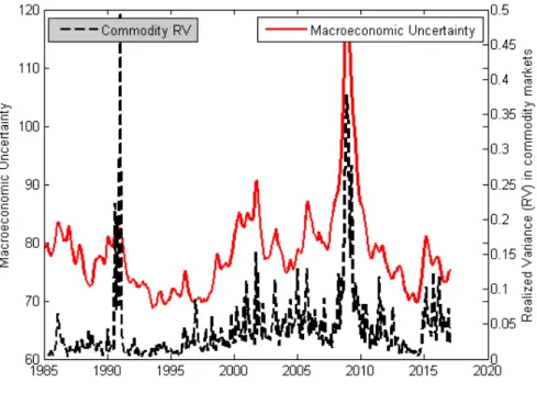
and FU indices. Moreover, Figures 1 and 2 below show the contemporaneous time
series movements of the Realized Variance (COMRV) of the commodity price index
and the MU and FU uncertainty series respectively.
[Insert Figure 1 Here] [Insert Figure 2 Here]
Figure 1 shows the contemporaneous movements of the JLN MU and the
Realized Variance (COMRV) in commodity prices. We can observe that rapid rises in
MU are being followed by jumps for the variance of the commodity price index and that the realizations of large shocks in the RV of commodity prices (e.g., the 2008-2009 volatility episode) are being followed by less uncertain (as indicated by a rapid
reduction in the MU index) macroeconomic environment. Figure 2 shows the
respective contemporaneous movements of the JNL FU index and the variance of the commodity price index. The relationship between FU and commodity price RV is similar with that of MU and RV, but there are some increases in the FU index which are not being followed by analogous jumps for the RV of commodity price index.
3.2 The Impact of Uncertainty Shocks on Commodity Price Volatility 3.2.1 The Impact of Unobservable Uncertainty Shocks
In this section we present the results of our multivariate (6-factor) VAR model in which we include as endogeneous variables the logarithm of the Manufacturing Industrial Production Index (MIPI)), the logarithm of the Manufacturing U.S. employment (MEMP)), the logarithm of the uncertainty index (log(Uncertainty) – MU, FU or EPU accordingly), the term spread (TERM) (the difference between the
12 In the appendix we additionally employ the same OLS regression models using the log of the
manufacturing Industrial Production and the Employment rate series, despite being I(1) processes, for robustness.
11
10-year U.S. government bond yield and the 3-month U.S. T-bill rate), the logarithm of the monthly price S&P500 index (SP500RV) and the Realized Variance of the
daily returns of Commodity Futures price index (COMRV)).13 The estimated 6-factor
model is inspired by the multivariate VAR models of Bloom (2009) and Baker et al.
(2016).14
The reduced form VAR model is given in Equation (2) below:
0 1 1 ...
t t k t k t
Y =A +A Y− + +A Y− +ε , (2)
where A0 is a vector of constants, A1 to Ak are matrices of coefficients and εt is the
vector of disturbances which have serially uncorrelated disturbances, zero mean and a variance-covariance matrix E( , )ε εt t' =σε2I.Yt is the vector of endogenous variables. All variables are in monthly frequency and cover the period from January 1985 until December 2016. The ordering in our 6-factor VAR model is as follows:
Yt =[MIPI MEMP MU TERM SPt t t t 500 t COMRVt]. (3)
Following the modeling approach of Bekaert et al. (2013), we choose to place
macroeconomic variables first and the financial variables (term srpead, stock-market, and commodity market) last in the VAR ordering selection due to more sluggish response of the former compared to the latter ones. We estimate a VAR model with 4
lags (k=4 in Equation (2)). The VAR(4) model is selected based on the Frechet and
the Akaike optimal lag-length VAR criteria.15Table 2, reports the Granger causality
13With the term ‘uncertainty’ we denote all the alternative economic uncertainty indices we employ in
order to measure the impact of the different indicators of economic uncertainty. Economic uncertainty refers both to macroeconomic and financial uncertainty. In our empirical analysis, in the main paper and the online appendix, we use six different indicators of economic uncertainty and five different indicators of financial uncertainty, thus, we estimate a total of ten multivariate VAR models.
14 Since we want to examine the impact of uncertainty shocks on the commodity price volatility, and
since the commodity prices are directly linked to the manufacturing production process, we choose to include the Manufacturing Industrial Production and Employment (instead of the respective aggregate figures for U.S. Industrial Production and Employment which are being used in the VAR model of Bloom (2009) and Baker et al. (2016)). Another minor difference is that instead of the Federal Funds Rate (FFR) and the logarithm of the Consumer Price Index (log(CPI)), we use the term spread which includes the expectations about the future level of short-term interest rates and inflation. In addition, in our baseline VAR model we exclude the wages and the working hours.
15We additionally run the VAR(3) model in order to compare the results with the VAR(3) model of
Baker et al. (2016). When estimated a VAR model with 3 instead of 4 lags, the main results and conclusions remain unaltered. The estimated IRFs for the VAR(3) model are provided upon request.
12
tests between the alternative proxies of economic uncertainty and the volatility of the commodity price index. The tests are conducted using the baseline 6-factor VAR model given in Equation (3), in order to control for different macroeconomic and financial shocks like the industrial production and the interest rates (term spread) shocks. We estimate a total of nine VAR models by placing the 9 alternative economic uncertainty proxies as the third variable of the VAR ordering (in the place of MU as shown in Equation (3)).
[Insert Table 2 Here]
From Table 2 we can observe that almost all proxies for economic uncertainty
Granger cause the Realized Variance of the commodity price index (COMRV). More specifically, the Financial Uncertainty (FU), the Macroeconomic Uncertainty (MU) and the Economic Policy Uncertainty (EPU) (and its main components) Granger cause the volatility of the commodity price index. In addition, the causality tests reveal a bi-directional causal relationship between commodity market volatility and the JLN Macroeconomic Uncertainty (MU) measure. The changes in the RV of
commodity price index cause changes in MU. On the other hand, as Panel C of Table
2 indicates, while the volatility in the S&P 500 index and the financial regulation
uncertainty (FRU) index have a causal effect in commodity market volatility, we fail to reject the hypothesis of no causality when conducting the test between the logarithm of the VXO index and the realized variance of the commodity market index (COMRV).
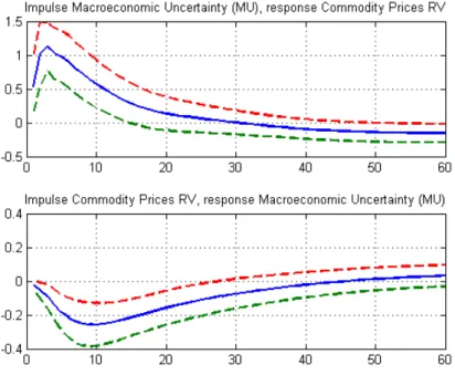
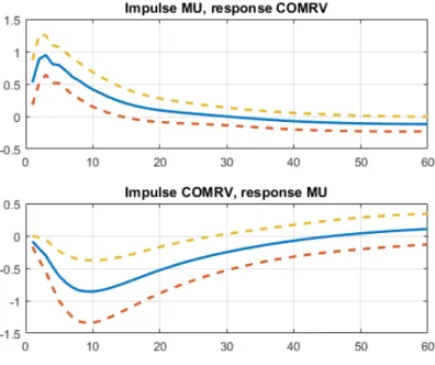
We continue the empirical analysis by measuring the impact of uncertainty shocks on the volatility of commodity prices. The impact of uncertainty shocks is quantified by estimating the Impulse Response Functions of the multivariate VAR model presented in Equation (3). More specifically, we base our analysis on the estimated IRFs between the logarithm of the various uncertainty indices and the realized variance of the commodity futures price index (COMRV). We firstly estimate the 6-factor VAR in which we use the unobserved proxy for macroeconomic uncertainty, i.e., the MU measure. The estimated Impulse Response Functions (IRFs)
13
between Macroeconomic Uncertainty (MU) and the Realized Variance of the
Commodity Futures price index (COMRV) are given in Figure 3.16
[Insert Figure 3 Here]
The estimated IRFs in Figure 3 show that a one percentage point (1%) shock in
Macroeconomic Uncertainty (MU) raises the monthly variance of the commodity price index (COMRV) by almost 1.1% for the first 3 months after the initial shock with the effect being positive and statistically significant for almost 15 months after the initial shock of uncertainty. In other words, we find that an increase in the JLN unobservable MU measure has a tremendous and long-lasting impact on the volatility of commodity prices. According to our VAR analysis, we are the first that provide evidence on the existence of common macroeconomic uncertainty factors which drive
the dynamics of the time-varying volatility in commodity prices.17 Our results are in
sharp contrast with the findings of the relevant literature (for example, Batten et al.,
2010), according to which there are no macroeconomic factors who can jointly influence the volatility of the commodity price series. On the contrary, our analysis reveals that the MU factor is a significant determinant of time-variation in the broad commodity futures price index.
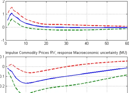
When examining the reverse channel of causality, we find that a positive shock in the realized variance (COMRV) of commodity prices reduces macroeconomic uncertainty (MU) in the short to medium run (2 months after the initial commodity volatility shock). The negative effect reaches its maximum 10 months after the initial commodity volatility shock and remains significant (i.e., statistically different from zero according to the bootstrapped 95% confidence interval) for about 25 months. The
16In our online appendix we report the estimated orthogonalized Impulse Response Functions in which
the shocks in the VAR model are orthogonalized using a Cholesky decomposition. According to Pesaran and Shin (1998), the generalized IRFs are invariant to the ordering of the variables in the VAR model, while the OIRFs are highly sensitive to the VAR ordering. For this reason, in our robustness section, we report the estimated OIRFs for different VAR orderings of the endogenous variables including in the VAR system. Following Pesaran and Shin (1998), we do not have to report the results of the estimated reduced form IRFs for different VAR orderings, since these IRFs are VAR ordering invariant. In addition, our results and basic conclusions remain unaltered when we estimate the OIRFs instead of the generalized ones. Koop et al. (1996) and Diebold and Yilmaz (2012) give further empirical support on these findings.
17 In the next paragraphs, we provide further robustness and empirical support to this finding. We show
that the MU shocks have a significant and long-lasting impact on the volatility of individual commodity prices (e.g., minerals and agricultural products), and not only on the variance of the broad commodity price index.
14
more sluggish response of macroeconomic uncertainty to changes in the volatility of commodity prices is somewhat expected. The economic interpretation of this negative response has its roots in the construction of the unobservable JLN macroeconomic uncertainty index. This index has been estimated as the purely unforecastable component of macroeconomic fluctuations, thus, when a large commodity volatility episode is materialized, the uncertainty (or the degree of unpredictability) in the macroeconomy falls because of the realization of the highly uncertain shock in the commodity markets. Our VAR analysis indicates that when a large shock in commodity markets materializes, then a large fraction of the foggy and uncertain state of the future path of the macroeconomy disappears. Our empirical findings show, for the first time in the literature, that the increasing volatility in commodity markets has significant bi-directional linkages with the time-varying degree of unpredictability in macroeconomic fluctuations.
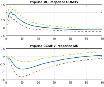
Moreover, we estimate the same 6-factor VAR model of Equation (1) with the Financial Uncertainty (FU) index instead of the Macroeconomic Uncertainty (MU) index. The Financial Uncertainty (FU) index (just like the MU index) is an unobservable uncertainty index which measures the degree of unpredictability in
financial markets. Figure 4 shows the estimated IRFs between the Realized Variance
(COMRV) in the Commodity Market index and the logarithm of the Financial Uncertainty (FU) index, along with the 95% bootstrapped confidence intervals.
[Insert Figure 4 Here]
From Figure 4 we can observe that an innovation in Financial Uncertainty (FU)
results to an instantaneous increase in commodity price volatility. More specifically, a 1% positive shock in FU results to a persistent increase in commodity market volatility which reaches its maximum (0.4%) in the first 5 months after the initial FU shock and remains positive and statistically significant (within the bootstrapped confidence interval) for 14 months after the initial shock. Our results, thus, indicate that both the JNL MU and FU shocks have a significant (in terms of magnitude) and long-lasting impact in commodity market volatility. In other words, when the future state of the macroeconomy and the financial system becomes foggier, the price variability in commodity markets increases as a response. Our VAR analysis additionally shows that the MU shocks have a more significant impact on the RV in
15
commodity markets when compared to the respective impact of FU shocks. Our results shows that the uncertainty about macroeconomic conditions seems to be the most important factor which drives time variation in commodity market volatility, when compared to the uncertainty about the conditions in financial system. In
addition, Figure 4 shows that the IRFs of FU to the commodity RV shocks are
statistically insignificant. These empirical findings show that, while macroeconomic uncertainty is significantly reduced after the occurrence of large volatility swings in commodity markets, the financial uncertainty remains unaffected and immune to changes in commodity market turbulence. Unlike the MU index, the FU index does not have a significant response to commodity market volatility shocks. The Granger
causality tests in Table 2 lead us to the same conclusion, since we confirm a
bi-directional causality between MU and Commodity market RV, and unibi-directional causality from FU to Commodity Market RV.
3.2.2 The Impact of Observable Uncertainty Shocks
In this section we present the results of our VAR analysis when we use some widely accepted proxies for economic uncertainty which are based on observable variations in variables which are closely connected to macroeconomic fluctuations and uncertainty. For example, Bloom (2009) proposes the stock-market uncertainty index (VXO) and the volatility of the S&P 500 price index (SP500RV) as proxies for
economic uncertainty. In addition, Baker et al. (2016) construct an Economic Policy
Uncertainty index (EPU) which quantifies the economic policy uncertainty and it is based on newspaper articles. The analytical methodology for the construction of the EPU index and its respective components (EPU news Policy Uncertainty index (EPUNEWS), Fiscal Policy Uncertainty Index (EPUFISC) and Monetary Policy
Uncertainty index (EPUMON)) can be found in Baker et al. (2016). Unlike the JNL
MU and FU uncertainty series, the EPU index, the VXO index and the realized variance of the returns of the S&P 500 index (SP500RV), are observable indicators of economic fluctuations and they may fluctuate for reasons which are uncorrelated with
economic uncertainty.18 Therefore, by estimating the impact of these alternative
18 Jurado et al. (2015) claim that “the stock-market volatility can change over time even if there is no
change in uncertainty about economic fundamentals, if leverage changes, or if movements in risk aversion or sentiment are important drivers of asset market fluctuations. Cross sectional dispersion in the individual stock returns can fluctuate without any change in uncertainty if there is heterogeneity in the loadings of the common risk factors.” In addition, Bekaert et al. (2013) give further empirical
16
uncertainty measures, we can empirically examine which type of uncertainty shock matters most for commodity investors and producers, the unobservable or the
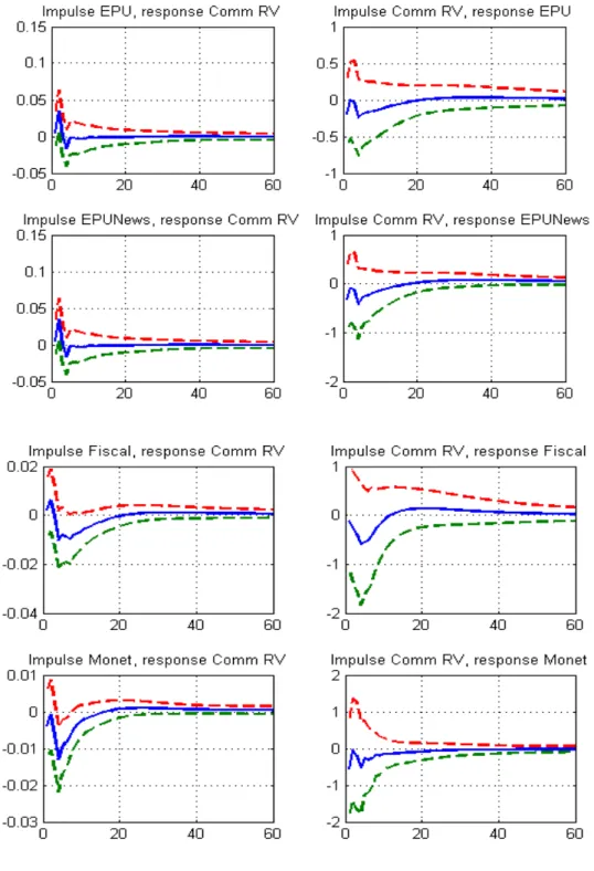
observable measure. Figure 5 shows the IRFs between the EPU index, as well as its
components, and the RV in commodity market index.
[Insert Figure 5 Here]
Both the magnitude and the responses of the Realized Variance of the commodity price index to EPU shocks are much smaller when compared to the respective response of the commodity price RV to MU shocks that was presented in
the previous section (Figure 3). For example, the commodity price index increases by
0.03% (3 basis points) in response to a positive 1% EPU shock. This effect is statistically significant only for the first month and vanishes after the second month. In addition, the response of commodity price volatility to the uncertainty about economic news (the news component of the Economic Policy Uncertainty index (EPUNEWS)) is of similar magnitude. These results show that, unlike the
stock-market volatility (Antonakakis et al., 2013;Liu and Zhang, 2015; Arouri et al., 2016),
the commodity market volatility seems to be relatively immune and less significantly affected by the observed uncertainty measures about future economic policy. Any kind of economic news which reveal a more uncertain economic environment, have a small and transitory impact on the volatility of commodity prices. In addition, the fiscal and the monetary policy components of the uncertainty index, have both a small negative impact on commodity price volatility. This negative impact of monetary (EPUMON) and fiscal policy uncertainty (EPUFISC) shocks vanishes after the second month of the initial shock.
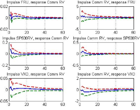
Moreover, we estimate the baseline VAR model of Equation (2), in which we use some additional proxies of economic uncertainty, which have been proposed in the relevant literature, such as the stock-market volatility of the S&P 500 index, the
VXO implied volatility index and the Financial Regulation index (FRU). Figure 6
shows the estimated IRFs for the commodity RV-uncertainty pair when we use the
support to this claim since they show that the time varying volatility (the VIX index) in the equity market can be decomposed to investor’s risk aversion and to economic uncertainty. This results show that the equity market volatility may change due to changes in risk aversion without any necessary change in the economic uncertainty.
17
RV of the S&P 500 index, the VXO index and the FRU index as alternative measures of uncertainty in the VAR model.
[Insert Figure 6 Here]
The stock-market volatility and financial regulation uncertainty shocks have positive, but small and transitory impact on commodity price volatility. For example, an one percentage point (100 basis points) shock in the logarithm of the VXO index increase the volatility in commodity prices by nine (0.09%) and two (0.02%) basis points respectively, with the effect being statistically insignificant. Overall, our results
cannot verify the volatility spillovers hypothesis (Arouri et al., 2011; Diebold and
Yilmaz, 2012). While for example, Diebold and Yilmaz (2012) find that there are significant volatility spillover effects from equity to commodity markets, our VAR analysis shows that the impact of stock-market volatility is transitory and small.
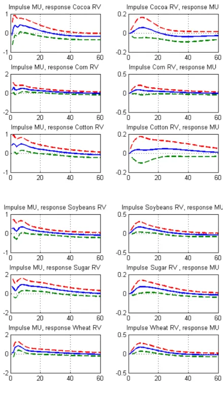
3.2.3 The Impact of Uncertainty Shocks on the Volatility of Individual Commodity Markets
In this section, we conduct a disaggregated VAR analysis in which we measure the impact of uncertainty shocks on the Realized Variance (COMRV) of individual commodity prices. Thus, instead of measuring the impact of the broad commodity price index, we measure the impact of uncertainty shocks on the volatility of various agricultural, metals and energy commodities. By this approach, we implicitly examine whether economic uncertainty is a common volatility risk factor in, not only the aggregate, but also the individual commodity markets. We estimate 14 models of our baseline VAR of Equation (2), in which we use the RV of each one of the 14 individual commodity prices instead of the broad commodity index. We employ the VAR analysis using the MU and FU measures as economic uncertainty proxies, since we have shown in the previous sections that the RV of the commodity price index has
an instant and highly persistent response to MU and FU shocks only.19 Figure 7
shows the estimated IRFs for the VAR models in which the volatility of the various
19For brevity, we do not report the responses of the volatility of commodity prices to EPU and
stock-market volatility shocks like we did in subsection 3.2.2 for the broad commodity price index. The responses to EPU and stock-market volatility shocks of the volatility series of individual commodities are found to be insignificant. These results can be provided upon request.
18
agricultural commodity prices are used as the endogenous variable and MU as the economic uncertainty measure.
[Insert Figure 7 Here]
The estimated responses of the volatility of agricultural products on the MU shocks are all positive and statistically significant. Our VAR analysis shows that an 1% MU shock results to an approximately 0.2-0.5% increase in the monthly Realized Variance (RV) of the agricultural commodity futures markets. This effect is persistently positive and reaches its maximum 2-3 months after the initial shock in all agricultural commodities under consideration. The estimated response of the RV of corn, wheat and sugar prices to an MU shock is more persistent (the effect remains statistically significant for many months after the initial shock). On the other hand, the IRFs show that the MU series is relatively immune to volatility shocks of agricultural commodities. The only exemptions are sugar and wheat which have a positive and
significant impact on MU. Figure 8 shows the estimated IRFs between
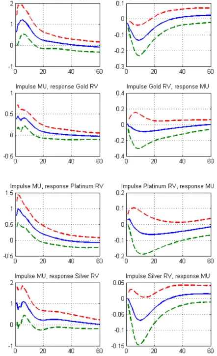
Macroeconomic Uncertainty (MU) and the Realized Variance in energy commodity markets.
[Insert Figure 8 Here]
The results indicate that the responses of the volatility of the energy commodity markets are more instant and long lasting when compared with agricultural markets. For example, a 1% MU shock results to a 2.5% increase in the volatility of crude oil price, and to a 2.2% increase in the volatility of heating oil price, with the effect being statistically significant from the first month until almost 18 months after the initial macroeconomic shock. In addition, a positive shock in the volatility of energy commodity markets reduces macroeconomic uncertainty. These results indicate a bi-directional causal relationship between energy commodity markets and macroeconomic uncertainty. These findings are in line with those of Hamilton (1983), Ferderer (1996), Hamilton (2003) and Elder and Serletis (2010) according to which oil price and volatility shocks are closely linked with the state of the macroeconomy
and are significant indicators of U.S. economic recessions. Finally, Figure 9 shows
19
[Insert Figure 9 Here]
The estimated IRFs from Figure 9 show that the effect of MU shocks in metals
markets is again positive and statistically significant. More specifically, our estimated IRFs show that a 1% positive MU shock results to an almost equal magnitude increase (about 1%) on the volatility of the copper, silver and platinum prices, with the effect being statistically significant for about 15 months after the initial MU shock. The effect of MU shocks is slightly lower on the volatility of gold prices. We have to state here that the impact of Financial Uncertainty (FU) shocks to the volatility of individual commodity prices is again significant, but of relatively less magnitude compared to respective impact of MU shocks. The results of our VAR analysis, in which we use the FU instead of the MU as endogenous variable in the VAR model for the agricultural, energy and metals markets, can be found in our online Appendix.
3.3 OLS Regression Models
In order to show the robustness of our VAR analysis, we additionally employ OLS regression models on the impact of economic uncertainty on the volatility of commodity prices. The estimated coefficients from these regressions provide an additional evidence of the impact of uncertainty shocks on the volatility in commodity markets. Overall, our regression analysis provides further empirical support to our findings, according to which the uncertainty shocks that matter most for commodity investors are the unpredictable ones. Here, we measure the impact of uncertainty shocks on the volatility of commodities, by regressing the alternative uncertainty measures on the realized variance of the commodity futures S&P GSCI market index
(COMRV). Table 3 reports the results of these univariate regression models in which
we use all the alternative, widely accepted, measures of economic uncertainty as explanatory variables.
[Insert Table 3 Here]
The results from Table 3 indicate that all economic uncertainty measures have a
20
price index, with the only exemption that of the fiscal policy uncertainty index. The insignificance of the fiscal policy uncertainty shocks is somewhat expected, since there is no empirical (or theoretical) evidence, linking commodity markets with fiscal policy. The coefficient of macroeconomic uncertainty (MU) is strongly positively significant and is much larger compared to the estimated coefficients of the other proxies of economic uncertainty. For example, the coefficient of the MU index is 0.359, while the estimated coefficients of the EPU and the VXO indices are 0.049 and 0.059 respectively. These results show the higher impact of MU on the realized
variance of the commodity price index.20 In addition, the adjusted R2 value of the
univariate regression model in the case of the MU index as the only determinant of
RV of the commodity price index, reaches 39.9%, while the respective R2 values for
the rest univariate models that uses alternative economic uncertainty proxies are less than 22%. Moving further, we control for several macroeconomic and stock-market variables, that have been proposed in the literature as determinants of commodity markets, and show that the large positive impact of economic uncertainty on commodity price volatility remains robust to the inclusion of these variables on the
left-hand side of our regression models.21Table 4 shows the estimated coefficients of
the multivariate OLS regression models.
[Insert Table 4 Here]
From Table 4 we observe that the estimated coefficients of MU and FU remain
positive and statistically significant, while the coefficients of the fiscal and monetary policy uncertainty become insignificant. Moreover, we employ a forecasting exercise in which we use the MU, FU and EPU series as predictors for the volatility of the commodity price index (COMRV). The forecasting regression model is given in the Equation (4) below:
20We have to state here that the significantly larger coefficients of the MU index do not result from a
different scale in the measurement of the alternative uncertainty measure. In order to have comparable results, we have multiplied the MU and the FU indices with 100 in order to be directly comparable and in line with the other economic uncertainty measures.
21For example, Arouri et al. (2011) report significant volatility spillovers from equity to commodity
markets, while Frankel and Hardouvelis (1985), Frankel (2008), Gilbert (2010) and Gubler and Hertweck (2013) identify the structural linkages between macroeconomic factors and commodity price and volatility dynamics.
21
COMRVt = +b0 b MU1 t k− +et. (4)
In Equation (4), MU represents the JLN macroeconomic uncertainty, but we employ the same regression model using the FU and the EPU uncertainty measures
for robustness purposes. Table 5 reports the relevant results. For brevity, we report
only the slope (b1) coefficients.
[Insert Table 5 Here]
The OLS regression results indicate that the MU and FU series are statistically significant predictors of the commodity price volatility for both short and long-term forecasting horizons ranging from one up to twelve months ahead. Unlike the MU and the FU measures, the EPU index gives statistically significant forecasts only for short-term (up to 3 months) forecasting horizons. Our empirical findings show, for the first time, the predictive information content of economic uncertainty measures on the volatility of commodity prices. Our results on the predictive power of the MU and FU series remain robust to the inclusion of various traditional determinants of the commodity price volatility like the interest rates, the growth in the manufacturing
Industrial Production Index and the volatility of the S&P 500 stock market index.22
4. Robustness
In the online Appendix we conduct various robustness checks to supplement our empirical results, following the VAR analysis and the OLS regression models of the main paper.
4.1 VAR Models
The Appendix provides additional robustness to our VAR results, by estimating the Orthogonalized Impulse Response Function (OIRFs) using a Cholesky decomposition and show the responces using the OIRFs instread of the Generalized IRFs which which we report in the main empirical section. Furthermore, we report the estimated OIRFs for alternative VAR orderings, following, for example, the VAR ordering of
22These results which provide robustness to the forecasting performance of the MU and FU series can
22
Bloom (2009) and Jurado et al. (2015), and we find that our results remain robust to
different VAR orderings. Moreover, motivated by the empirical studies on the
significance of exchange rates (Gilbert, 1989; Chen et al., 2010) and crude oil price
shocks (Du et al., 2011; Nazlioglu and Soytas, 2012; Shang et al., 2016) for the price
and the volatility path of commodities,we additionally control for the U.S. effective
exchange rate and the oil price shocks in our VAR model. Lastly, we report the Granger causality tests between the uncertainty measures and the realized volatility of agricultural, energy and metals prices and find that there is a bi-directional causality between MU and the volatility in energy markets, while there is a unidirectional causality from MU to the volatility of agricultural and metals prices. Lastly, our VAR models and Granger causality reveal a significant impact of FU shocks on the volatility of agricultural, metals and energy futures markets.
4.2 OLS Regression Models
The Appendix contains various robustness checks to the OLS regression models of the main paper. More specifically, in order to provide further robustness to our OLS estimates which are presented in Section 3.2, we employ the same regression models in which we use the log-levels instead of the log-differences of the manufacturing IPI and the manufacturing Employment. In this way, we use exactly the same explanatory variables in the regression models as with the VAR system and we show that our empirical results remain unaltered, and are unaffected by the stationarity condition of these two variables (I(0)/I(1)). We, additionally, apply the same OLS regression models in which we use the JLN macroeconomic and financial uncertainty series which have 1, 3 and 12 month forecasting horizons (i.e., the MU1, MU3 and MU12 and the FU1, FU3 and FU12 respectively). By this exersise we empirically verify that both MU and FU series have a significant impact on the commodity price volatility irrespective of the forecasting horizon that has been used for their construction. Furthermore, we run the OLS regression models and we additionally control for the exchange rate and crude oil shocks (for consistency reasons, the left-hand side variables in these regressions are similar with those that are included as endogeneous variables in our 8-factor VAR model). These results show that the impact of MU and FU shocks remains nearly the same under this regression specification with that of our
23
sluggish (and not contemporaneus) reactions of commodity markets to uncertainty shocks, we use the same OLS regression models of the Subsection 3.3 in which here we include the lagged (one month before) explanatory variables. These results provide further evidence regarding the persistence of the impact of uncertainty shocks on commodity market volatility. These findings can alternatively be viewed as a first indication of the forecasting power of the JLN economic uncertainty measure on the commodity price volatility. Lastly, we empirically show that the impact of MU and FU shocks on the volatility of individual commodity prices is robust to the inclusion of additional macroeconomic factors (like the oil price shocks and the exchange rates) which are found in the literature that are directly linked to the commodity price volatility.
4.3 Uncertainty Shocks During the Financialization Era
In this section of the Appendix, we conduct the empirical analysis for the post-2000 period, during which the financialization of commodities (i.e., a large inflow of investment into commodity markets) has taken place. The financialization of commodity markets has led to structural changes in the nature as well as their information content. Since the early 1990s, the large inflow of funds and the increased presence of financial investors in commodity markets have transformed commodities into a separate asset class which has become more integrated to the rest of the financial markets (see Irwin and Sanders, 2012; Cheng and Xiong, 2013;
Silvennoinen and Thorp, 2015; Basak and Pavlova, 2016). Tang and Xiong (2012)
find that the financialization of commodity markets lies behind the increased (post-2008) correlation of oil prices and non-energy commodity prices, and the increased volatility of non-energy commodities around 2008. Motivated by the empirical findings that show an increased interdependence between stock-market and commodity market returns during the financialization period (Buyuksahin and Robe, 2014; Adams and Gluck, 2015), we empirically examine whether the financialization process has increases the structural linkages between uncertainty shocks and commodity market volatility.
Our empirical results indicate that the financialization in commodity markets has increased the interdependence and the sensitivity of commodity market volatility to uncertainty shocks. We show that the explanatory power and the significance of all
24
the economic uncertainty measures have tremendously increased during the post-2000 period. These results contradict with those of Karali and Power (2013) who find that the commodity specific factors dominate the macroeconomic factors when they are used to explain the volatility during the recent 2006-2009 period in the U.S. agricultural, energy and metals futures markets. On the contrary, our econometric analysis reveals that the common macroeconomic uncertainty factor explains a larger part of the time variation of the commodity price volatility in the post-financialization era, while this is not the case in the pre-2000 period. In order to provide robustness to our evidence regarding the significance of the financialization period, we run the same regressions for the pre-financialization (pre-2000) period. The results for the pre-2000 period provide robustness to our findings, since we show that most of the economic uncertainty measures turn from significant to insignificant during the pre-2000 period. These results can be found in the online Appendix.
5. Conclusions
This paper investigates the impact of uncertainty shocks on commodity price volatility. Overall, our results show that macroeconomic uncertainty increases volatility in commodity markets. Our analysis indicates that the rising degree of unpredictability in the macroeconomy, which is proxied by the latent uncertainty
measure of Jurado et al. (2015), has the most singificant and persistent impact on the
volatility of commodity prices. On the other hand, the observable economic uncertainty measures have a rather transitory and less significant impact on the volatility of commodity prices. Our results suggest that the more unpredictable the future state of the macroeconomy becomes, the more volatile the prices of commodities will be.
The policy implication behind these findings is that the adoption of appropriate monetary and fiscal policies that can lead to the reduction of the unpredictability of macroeconomic fluctuations, will reduce also the variability of commodity markets. Commodity market turbulence does not seem to arise because of the per se macroeconomic and/or stock-market fluctuations. On the contrary, it is affected by the rising degree of unpredictablility of these fluctuations. Any macroeconomic policy that can result in reducing this unpredictability (e.g., an adoption of a highly transparent monetary policy), will implicitly reduce the fluctuations as well as the
25
instability in commodity prices. Our VAR and OLS regression models indicate that the JNL macroeconomic uncertainty proxy, explains a large part of the time-varying volatility in commodity markets and, in addition, has a high predictive power when is used as a volatility predictor into the left-hand side of our volatility forecasting OLS regressions.
This paper examines the impact of economic uncertainty on the volatility of commodity markets through a unified framework employing both observable and unobservable macroeconomic and financial uncertainty shocks. One direction for future research would be the empirical examination of the predictive power of economic uncertainty on the volatility of commodity prices. We believe that it would be of interest to examine the predictive information content of macroeconomic uncertainty, when compared to the already empirically verified specific predictors of volatility in commodity markets (e.g., the inventory level and the option-implied volatility). This information would be very useful for commodity investors, producers and trade-policy makers.
References
Adams, Z., and Z., Gluck (2015). “Financialization in commodity markets: A passing trend or the new normal?” Journal of Banking and Finance, 60, 93-111.
Antonakakis, N., Chatziantoniou, I., and G., Filis (2013). “Dynamic co-movements of stock-market returns, implied volatility and policy uncertainty.” Economics Letters, 120, 87-92. Anzuini, A., Lombardi, M.J., and P., Pagano (2013). “The impact of monetary policy shocks on commodity prices.” International Journal of Central Banking, 9(3), 125-150.
Arouri, M., Estay, C., Rault, C., and D., Roubaud (2016). “Economic policy uncertainty and stock markets: Long-run evidence from US.” Finance Research Letters, 18, 136-141.
Arouri, M., Jouini, J., and D.K., Nguyen (2011). “Volatility spillovers between oil prices and stock sector returns: implications for portfolio management.” Journal of International money and finance, 30(7), 1387-1405.
Baker, S.R., Bloom, N., and S.J., Davis (2016). “Measuring economic policy uncertainty.” Quarterly Journal of Economics, 131(4), 1593-1636.
Basak, S., and A., Pavlova (2016). “A model of financialization of commodities.” Journal of Finance, 71(4), 1511-1556.