EXPERIMENTAL AND NUMERICAL STUDIES ON DOUBLE DELTA WING WITH SHARP LEADING EDGE AT SUBSONIC SPEED

(1)

EXPERIMENTAL AND NUMERICAL STUDIES ON DOUBLE DELTA WING

WITH SHARP LEADING EDGE AT SUBSONIC SPEED

Yuvaprakash J

1

, P. Kumar

2

, S. Das

3

and J.K. Prasad

4

1

_{Department of Space Engineering and Rocketry Birla Institute of Technology, Mesra, Ranchi}

---*---Abstract -**

An attempt has been made to investigate the

flow field characteristics of double delta wing both numerical and experimental at different angles of attack ranging from 0 degree to 30 degrees. In this research a sharp leading edge double delta wing with 810_/450_{sweep angles were analyzed,}

experimentally with subsonic wind tunnel facility and numerically with Fluent software, both using Quantitative techniques like force, static pressure measurement and Qualitative techniques like oil flow visualization. A grid independence study has been carried out. S-A turbulence model is used for computational studies. The results were compared to understand the effect of angle of attack on vortex formation, breakdown location and separation.

Key Words: Double delta, Vortex breakdown, Separation,

Leading edge.

1.INTRODUCTION

An understanding of the vortical structures and vortex breakdown location, separation is essential for the development of highly maneuverable and high angle of attack flight, this is primarily due to the physical limits these phenomena impose at extreme flight conditions. Modern aircrafts have the ability to fly at high altitude and attain high angles of attack. But increasing the angle of attack leads to the existence of very complicated flow structures around the body. The rapid advancement of flight vehicle technology has resulted in a substantial increase in the complexity of aerodynamic designs and corresponding flow fields. The interest in double delta wing stems from its natural characteristic to generate leading edge strake-wing vortices. These vortex flows can contribute crucial effect to manoeuver aerodynamics. The fundamental understanding and predictability of the onset of flow separation are of paramount importance to almost every aspect of flight aerodynamics, regardless of vehicle class and flight envelope.

Presented at 27th National convention of Aerospace Engineers, Institution Engineers, Dehradun, November’13.

The occurrence of separation induced leading edge vortex flows over an airborne vehicle, if not controlled, can have a significant adverse effect on the aircraft aerodynamic performance, stability and control characteristics. Prediction of aircraft aerodynamics with this separated flow over the wing depends on many parameters such as Reynolds number, Compressibility, finite wing leading edge bluntness, Mach number and many other factors. Majority of the flight time for aircraft is spent at subsonic speeds and that is why the study at low speeds gain importance.

1.1.Double Delta Wing

Double delta wing planforms incorporate two distinct leading edge sweep angles. The first part of is the strake, has a much higher sweep angle than the aft portion of the wing,

the

main wing.

At low angle of attack, two primary vortices originating from the strake and wing leading edge remain distinguishable over the entire wing. At moderate to high angles of attack, theflow over such wings separates at the leading edges, resulting in a steady and stable so called leading edge vortex flow, merge into one stable vortex downstream. At high angle of attack, double delta wing can generate higher lift than rectangular wings, with better aircraft stability and control characteristics. Vortices will merge right after the kink and are no longer separated. At very high angle of attack (nearstall) the large scale vortex breakdown occurs inevitably over the wing. The vortices originating from the highly swept strake can stabilize the leading edge vortices emanating from the main wing. These concentrated leading edge vortices generate very low pressure levels on the wing surface directly below the vortical cores and hence result in a large normal force. However, above a crucial angle of attack, the vortices are no longer stable and well defined.

(2)

1.2.Flow Physics

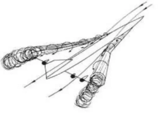
In recent years several experimental investigations on double delta wings have been carried out. A typical sketch of flow pattern over double delta wing is shown in Fig 1.1. The flow over strake is similar to that around a straight leading edge delta wing. At low angles of attack, two primary vortices originating from the strake and wing leading edges are shed leeward on each side of the wing and remain undistinguishable over the entire wing. At medium angles of attack, the vortices merge into one stable vortex over the rear part of the wing. At high angles of attack, the large scale vortex breakdown occurs inevitably over the wing. The leading edge vortex, which is characterized by high velocities and low static pressure, increases in diameter and intensity as the core follows a path downstream and inboard at an angle slightly greater than the sweep angle. As the angle of attack is increased, the vortex axial and rotational velocities increase and the vortex core height above the wing increases and the core moves inboard. Primary vortex generation is nearly independent of Reynolds number due to extremely small effective length or radius of curvature of the leading edge. However, high Reynolds number flow does decrease vortex diameter because it effectively adds energy and velocity to the core resulting in a more tightly wrapped core. Unlike the primary pair, the secondary vortex pair’s strength and size are dependent on Reynolds number. Strength of the secondary vortex is then a function of area covered by and velocity of the lateral boundary layer flow. Fig 1.2 shows the vortical flow pattern at leading edge of the sharp double delta wing.

Fig 1.1: Flow over Double Delta Wing

Fig 1.2: Vortical flow pattern – Leading Edge

1.3.Vortex Breakdown Characteristics

The geometry of these wings further complicates the flow field structure due to the presence of the pair of coherent vortices produced by the strake and wing leading edges. The strake vortices beyond the kink tend to remain fairly constant as they are no longer being fed energy from flow separation over the main wing. They typically move outboard and closer to the surface of the wing. The main wing vortices are more highly energized and tend to move inwards and away from the surface of the wing. If the leading edge is sharp the flow will separate along its entire length.

Vortex breakdown occurs when the vortices begin to fall apart from a rapid expansion when the wing reaches a critical angle of attack. Once the vortices begin to deteriorate, the pressure distribution over the wing changes and the result is a reduction of the lift curve slope. A further increase in angle of attack from this point forward causes the breakdown location to move aft towards the trailing edge. Wings with a leading edge sweep greater than 75-deg, the maximum lift is realized at the trailing edge and the wing stalls when the breakdown location increases beyond this point, vortices go under a transition process (undergo a sudden expansion) known as vortex breakdown. The reattachment location on the wing surface moves inboard with increasing angle of attack and reaches the wing centerline at particular incidence. Beyond this limiting angle of attack, flow reattachment to the wing surface is not possible. The shedding, interaction and breakdown of these vortices are highly sensitive to both the aircraft’s geometry and the flow conditions. In addition to producing the benefits of enhanced lift and maneuverability, the vortical flow also causes serious flight path departure and structural fatigue problems. The magnitude of the lift and pitching moment decreases after vortex breakdown. There are two important parameters affecting the occurrence and movement of vortex breakdown: swirl level and pressure gradient affecting the vortex core. An increase in magnitude of either parameter promotes the earlier occurrence of breakdown. Fig 1.3 and 1.4 shows the topology of cross flow over the wing and effect of angle of attack on double delta wing.

(3)

Fig 1.3: Topology of cross flow over wing

Fig 1.4: Effect of angle of attack

2.RESEARCH METHODOLOGY

2.1.Experimental Work

Qualitative and Quantitative analysis were made in orderto obtain the overall flow field around a double delta wing at varying angles of attack. Qualitative analysis included the oil flow visualization and Quantitative analysis included the measurement of force using strain gauge balance and measurement of surface static pressure. The details of the test facility, experimental model and mounting arrangements, instrumentation and the method of testing are given in the following sections.

2.2.Wind Tunnel Description

Experiments were carried out in the low speed subsonic wind tunnel facility which has a test section size of 600 mm x 600 mm. The length of the test section is 1200 mm. It is an open circuit continuous flow wind tunnel in which air is sucked by a propeller located at the aft section of the tunnel. Experiments were carried out at a Reynolds number of

2×105_{and at a velocity of 17 m/s. A schematic showing the}

details of the tunnels is shown in Fig. 2.1.

Fig 2.1: Layout of wind tunnel

2.3.Test Model details

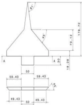
Model is made out of aluminium. The double delta wing has a strake/wing sweep angle of 81/45 deg sharp leading edge, thickness of 8.6 mm, chord and span are 179 mm and 169 mm. Two different models have been made in order to obtain the forces and pressures. The dimensional details of the model (in mm) are shown in Fig 2.2.

(4)

Suitable incidence was chosen in order to vary the angles of attack of double delta wing in the pitch plane. The

incidence had an accuracy of + 0.050_{and was fully}

automated. It was assumed that the model after mounting and during the run conditions had no vibrations. The incidence mechanism was controlled using a DC motor drive

and DAQ system (NI). The model pitched from 00_{to 30}0_in

steps of 50_.

2.4.Data Acquisition system

All the data were acquired using DAQ system provided by

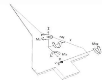
National Instruments. An 80 channel card was used to obtain the pressure from pressure sensors. Signal conditioner (NI) and 16 channel ADC (analog to digital converter) card was used to obtain the forces. Signal conditioner had the capability to filter the noise levels from 10 Hz to 10 KHz. Forces and moments acting on the double delta wing is shown in Fig 2.3:

Positive X is the axial force. Mx is the rolling moment. Positive Z is the normal force. Mz is the yawing moment. Positive Y is the side force. My is the pitching moment.

Force measurement was done by using 5-component strain gauge balance along with the data acquisition system using LABVIEW software. A 3 volt DC was used to excite the strain gauge balance. The balance works on the principle of wheat stone bridge. Strain gauges mounted on balance are strained due to force leads to change in electrical resistance of the gauge which is proportional to the strain produced. The four gauges are connected to one arm of Wheatstone bridge to measure the voltage due to strain which could be further converted to obtain the force using coefficient matrix. The voltage obtained is further post processed in order to obtain coefficients of forces and moments. A typical force measurement system with internal strain gauge balance attached to the double delta wing model is shown in Fig 2.4.

Fig 2.3: Coordinate system for forces and moments

Fig 2.4: Model with internal strain guage

2.5.Principle of Strain Measurement

Strain initiated resistance change is extremely small. Thus for strain measurement a Wheatstone bridge is formed to convert the resistance change to a voltage change. Here R1, R2, R3, R4 are the resistances and the bridge voltage is (V) is E. then, the output voltage is given by (V0) as,

V0 =

Suppose the resistance R1 is a strain gauge and it changes by ΔR due to strain. Then, the output voltage is,

V0=

Thus obtained is an output voltage that is proportional to a change in resistance, i.e. a change in strain. This very low output voltage is then amplified for analog recording or digital indication of the strain.

2.6.Estimating Forces

All the data from strain gauge balance were obtained inthe form of matrix and it was multiplied to the coefficient matrix supplied by the manufacturer to obtain the forces.

[O] = [A] [F]

[F] = [A]-1

[O]

[O] = output matrix (in milli volts) [A] = coefficient matrix

(5)

From those values the coefficient values are obtained by using the following formulas.

N = N1 + N2 A = A1 + A2

Cn = and Ca =

2.7.Calculation of Moments

Moments acting on double delta wing with respect to c.g of the wing are taken. The following formulas were used to get the required values and their values are plotted.

N0 = N1 + N2 My0 = (N1 – N2) × 50 Mycg = My0 + (N0 × L)

2.8.Static Pressure Measurements

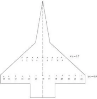
Static pressure tapping were made at different x/c locations over the model by making holes of 1.3 mm diameter drilled normal to the surface of the model. Steel tubes of 1.2 mm diameter, are then connected to polythene tubes to the pressure tapings that were made on the surface of the model. The data from the pressure sensor box were acquired through a data acquisition system and Lab view software. This provides voltage output proportional to pressure applied. The voltage output from the sensor is read and system converts the voltage into pressure via a calibrated chart. A schematic of model used for pressure measurement is shown in Fig 2.5.

Fig 2.5: Schematic of model showing pressure ports at stations x/c = 0.7, 0.9

3.COMPUTATIONAL WORK

In the present study, computation has been done using Fluent. Mesh was generated using Gambit. Model is designed in Catia software. PROCEDURE  Pre processing   Solution   Post processing   3.1.Pre Processing 3.1.1.Grid Generation

Grid generation is done using Gambit. A 3-D structured grid was generated around the wing with spherical O-O domain 15c the body (15 times the root chord). First length option was used with 0.01c. Mesh was generated using Quad and map option for structured grid. The flow field variables were solved by means of cell based scheme.

3.1.2.Boundary Conditions

A free stream condition was given at the inlet and the downstream values were extrapolated from the interior solutions. Fig 3.2 shows the computational domain for the double delta wing. The front portion of the sphere was considered as velocity inlet and aft portion was considered as outflow. The body was considered as wall. No-slip wall conditions are applied to the model surfaces without any wall roughness. Free stream velocity directions are adjusted in accordance to the imposed angle of attack and sideslips for different simulation run. The solution is initialized uniformly with the free stream condition throughout the domain.

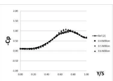
3.1.3.Grid Sensitivity/Independence Study

A grid independence study was conducted for the model dimensions in Ref [2]. Three different grids with 0.4 million, 0.5 million, 0.6 million cells (with first cell length 0.01c as constant) and Two different grids with 0.01c and 0.05c (c - root chord) first cell length (0.6 million) were considered for this study. This variation in number of cells was obtained by varying the growth rates. Fig. 3.3 (a) and (b) shows the

pressure distribution curve for α=120_{at x/c = 0.55 and x/c =}

0.75 with different cell counts. Fig 3.4 (a) and (b) shows the

pressure distribution curve for α=120_{at x/c = 0.55 and x/c =}

0.75 for different first cell length. All the test cases were shown similar trend and values. Finally the grid with 0.6 million cells and 0.01c is adopted for all further computational studies.

(6)

Fig 3.1: Surface grid generated over the model

Fig 3.2: Structured grid with spherical domain

Fig 3.3: (a) Grid independence - cell count at x/c = 0.55

Fig 3.3: (b) Grid independence - cell count at x/c = 0.75

Fig 3.4: (a) Grid independence - cell length at x/c = 0.55

(7)

3.2.SOLUTION

Once a suitable mesh has been generated, a computational algorithm numerically solves the equations for fluid properties values at each volumetric cell center, from which these values can be interpolated to cell faces. Computations may cease once the solution has converged or has come to fully developed flow. Fluent uses the complete mesh flexibilities to study the structured mesh about any geometry in any domain to analyze the flow. It is based on the Finite Volume Method. For the present study segregated, laminar/S-A, unsteady, incompressible, second order implicit and second order upwind for momentum is used.

The case was solved for 0.3 seconds with a global time

step of 0.001 (10- 3_{) in unsteady. Boundary conditions like}

velocity inlet for the inlet, outflow for the outlet, wall for model is given and all cases were run with velocity of 17 m/s. Fig 3.5 (a) and (b) shows the total pressure contour at x/c = 0.55 and x/c = 0.75 with comparison between Ref (2) and present computation results.

Fig 3.5: (a) Comparison of total pressure contour at x/c

= 0.55 (α=120_{) between Ref (2) and present computation}

Fig 3.5: (b) Comparison of total pressure contour at x/c =

0.55 (α=120_{) between Ref (2) and present computation}

3.2.1.Turbulence Model

Spalart-Allmaras turbulence model is used for the present study. This a relatively simple one equation model that solves a modeled transport equation for the kinematic eddy viscosity. This model is effectively a low Reynolds number model, requiring the viscous affected region of the boundary layer to be properly resolved. In fluent, however, the model has been implemented to use wall functions when the mesh solution is not sufficiently fine. This might make it the best choice for relatively crude simulations on coarse meshes where accurate turbulent flow computations are not crucial. Furthermore the near wall gradients of the transported variable in the model are much smaller than the gradients of the transported variable in the K-ε and K-ω models. This might take the model less sensitive to numerical error when non-layered meshes are used near walls.

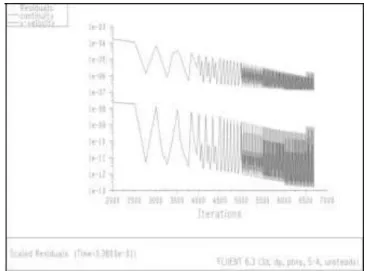
Fig 3.6 shows the typical convergence graph for S-A turbulent case.

Fig 3.6: Residual plot showing continuity and x-velocity

3.3.Post Processing

After the pre-processing, the simulation setup can be stored as a case and data file. The case file includes the information for the grid, the boundary conditions and the solver settings. The data file stores information about the data in each node of the cells. The contour plots, vector plots and the surface data plots etc. of pressure, velocity and density etc. can be checked during the solution process and at convergence. These plots can be saved as image files and the data from surface plots can be written on to a file and plotted. Points, lines, rakes and planes can be created in the flow domain to analyze the properties at the desired locations.

(8)

A graph between Cp and x/c locations is plotted for different angle of attack. Several things like vorticity, total pressure, velocity contour are also visualized to understand the nature of strake and wing vortex, vortex breakdown location etc.

4.RESULTS AND DISCUSSION

The results obtained through force, static pressure and oil flow visualization are discussed in the subsequent sections to understand the effect of angle of attack on vortex formation, breakdown location, separation and pressure distribution over the body at specified locations. The experimental results are compared with the computations.

4.1.Aerodynamic Force Measurement

Five component strain gauge balance has been used to measure the force and moments.

Fig 4.1 shows the variation of normal force with increase in angle of attack. The normal force seems to be almost

linear up to α = 300_{. Further increase in angle of attack keeps}

the normal force fluctuating about a certain value. The point from which the normal force seems fluctuating is known as stall point.

Fig 4.2 shows the variation in axial force coefficient with angle of attack. The axial force seems to be lies within the

range of 0 to +0.2 up to α = 300_{. No drastic variation in axial}

force can be noticed throughout. Variation in angle of attack seems to have only very less effect on axial force value unlike normal force which is increasing linearly with angle of attack.

Fig 4.3 shows the variation in lift force coefficient with angle of attack. At 0 degree angle of attack we can see the positive lift force. The lift force seems to be linear up to α =

300_{with range of values from 0 to +1.2. Further increase in}

the angle of attack keeps the lift force fluctuating about a certain value. The point from which the lift force seems fluctuating is known as “stall point”.

Fig 4.4 shows the variation in drag force coefficient with angle of attack. Drag is generated by every part of the model due to the interaction of fluid over a solid body. Thus we can find a positive value of drag force coefficient at 0 degree angle of attack. At lower angles of attack the drag force is mainly due to skin friction. Therefore the value of drag force

coefficient rises very slowly till α = 150_{. After which induced}

drag (drag due to lift) occurs, because the flow near the wing tips is distorted span wise as a result of the pressure difference from the top to the bottom of the wing. The local angle of attack of the wing is increased by the induced flow of the tip vortex, giving an additional, downstream-facing component to the aerodynamic force acting on the wing.

The values obtained through computation are following the same trend with the experiment throughout the graph plotted till higher angles of attack. The percentage of error is remained same for whole process may be due to minor errors which could be due to insufficient grids. The trend of graph is same for both experiment and computation which shows very good agreement in results.

Fig 4.1: Comparison of Normal force coefficient

(9)

Fig 4.3: Comparison of Lift force coefficient

Fig 4.4: Comparison of Drag force coefficient

4.2.Static Pressure Measurement

The Cp versus y/s has been plotted for different axial locations. The overview of graph plots shows that as the angle of attack increases, suction pressure increases to some extent after which it stalls.

At low angle of attack (α = 00_{, 10}0_{at x/c = 0.7, 0.9) Fig 4.5}

to 4.8 shows that the contribution from strake vortices towards suction pressure can’t be noticed well when compared with the wing vortices. Vortices are symmetry in nature. Only wing vortices can be seen. At low angles of attack very negligible strake effect is observed.

At medium angle of attack (α = 200_{at x/c = 0.7, 0.9) Fig}

4.9, 4.10 shows the separate strake and wing vortices with little symmetry nature. Contribution from strake vortices has increased considerably which can be noticed by a little peak near to the axis which provides additional lift force which is an added advantage when compared to the delta wing. The suction pressure peak for both strake and wing vortices is comparatively higher in x/c = 0.7 than at x/c = 0.9 which may be due to vortices breakdown and interaction near the axis.

At high angle of attack (α = 200 at x/c = 0.7, 0.9) Fig 4.11,

4.12 shows the asymmetric nature of vortices and pronounced peak in suction for strake vortices and the magnitude is comparatively higher. Wing vortices contribute largely towards suction at all angles of attack. The suction pressure peak for both strake and wing vortices is comparatively higher in x/c = 0.7 than at x/c = 0.9 which may be due to vortices breakdown and interaction near the axis. The values of strake and wing vortices peak is relatively less when compared to medium angle of attack.

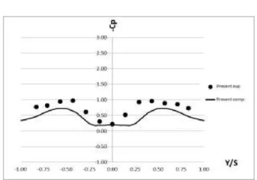
Fig 4.13 and 4.14 shows the effect of angle of attack on double delta wing at x/c = 0.7, 0.9.

The trend of graph is same for both experiment and computation showing very good agreement in results at x/c =0.7 and acceptable result at x/c = 0.9. Only at higher angle of attack very little difference between computation and experiment can be noticed. May be an additional finer grid packed closely around the body and use of other turbulence models will get good results, but it is currently limited by available computing power.

(10)

Fig 4.6: Comparison of Cp at x/c = 0.7 for α = 100

(11)

Fig 4.13: Effect of angle of attack (α) at x/c = 0.7

Fig 4.14: Effect of angle of attack (α) at x/c = 0.9

4.3.Oil Flow Visualization

Comparison between experiment (left-half) and computed (right- half) oil flow over the surface of double delta wing from 0 to 30 degrees (in order of 10).

Fig 4.15 shows the comparison at α = 00, in which no

appreciable vortices pattern can be seen distinguishably. Only we can identify the flow distortion on both computation and reference near middle of the wing.

Fig 4.16 shows the comparison at α = 100, in which we are

able to see the markings of strake and wing vortex regions and distorted flow near tip of the wing. Similarly even in computation continuous lines are seen in the region of vortex and distorted region is visible near tip of the wing. Strake and wing vortices are very clearly distinguishable.

Fig 4.17 shows the comparison at α = 200, we can observe

both strake and wing vortex starting from leading edges of the wing and getting merged somewhere near the middle of the

wing. Even though in computation strake vortex and wing

vortex are not so clearly visible we can identify the similar region like vortex from leading edge to middle of the wing.

Fig 4.18 shows the comparison at α = 300, we can observe

both strake and wing vortex are not clearly distinguishable, both of them merges together and no longer separate.

(12)

Fig 4.16: Comparison of oil flow at α = 100

4.4.Vorticity Contour

Fig 4.19 shows the computed vorticity contour at α = 00

at x/c= 0.5, 0.7, 0.9. No much appreciable visibility of vortices at all locations.

at x/c= 0.5, 0.7, 0.9. As the angle of attack is increased we can see the formation of circulation zone which in turn represents the initialization of vortex. Still two contours are not interacting.

at x/c= 0.5, 0.7, 0.9. As the angle of attack is further increased we can see the increase in vorticity contour size and towards the station x/c = 0.9.

at x/c= 0.5, 0.7, 0.9. As the angle of attack is further increased we can see the increase in vorticity contour size and towards the station x/c = 0.9 and we can see that vortices started interacting with each other near the middle axis.

Fig 4.19: Vorticity contour at x/c = 0.5, 0.7, 0.9 at α = 00

(13)

4.5.Path Lines

Fig 4.23 shows the computed path line at α = 00. No

strake or wing vortices can be seen. The flow is still attached to the body.

Fig 4.24 shows the computed path line at α = 100. We can

observe that both strake and wing vortex starting from leading edges of the wing and are separate and clearly distinguishable.

observe both strake and wing vortex starting from leading edges of the wing and getting merged somewhere near the middle of the wing, but we can distinguish them to some extent.

observe both strake and wing vortex are not clearly distinguishable, both of them merges together and are no longer separate.

Fig 4.23: Computed Path lines at α = 00

(14)

5.CONCLUSION

A number of important conclusions have been made from the present investigation. At low to moderate angle of attack, symmetric flow across the root chord was observed and confirmed through both computation and experiment. At higher angle of attack asymmetric nature of vortices across the root chord was seen. As the angle of attack increases, the size and strength of vortex is increasing up to critical angle. With the increase in angle of attack there is an upstream progression of the strake-wing vortex separation. At high angle of attack better formation of secondary separation line and vortex attachment is realized. It is observed that at a given x/c, magnitude of strake and wing vortex suction peak

increases up to α = 200_{. Due to vortex breakdown, the}

magnitude of strake and wing vortex suction peak decreases at high angle of attack. Normal force values and pressure suction peaks are well justified by the S-A turbulence model, whereas Kω-SST model gives comparatively lower value and similarly for other models of turbulence. Comparing with the previous experiments conducted on round edged double delta wing based on literature, normal force is less at similar angle of attack for the sharp edged model.

REFERENCES

[1] Verhaagen N.G, Jenkins L.N, Kern S.B, Washburn A.E,

“A Study of the vortex flow over 76/40 deg double delta wing”, ICASE report no 95-5, Feburary 1995.

[2] Hsu C.H and Liu C.H, “ Navier stokes computation of

flow around a round edged double delta wing”, Vol 28, no 6, AIAA Journal, June 1990.

[3] Al-Garni, A.Z Saeed and Al-Garni A.M, “Experimental

and Numerical Investigation of 65-deg delta and 65/40-deg double delta wings”, Journal of Aircraft, log number C10913.

[4] Verhaagen N.G, “Effect of Leading edge radius on

Aerodynamic characteristics of 50-deg delta wings”, AIAA 2010-323, 4-7 January 2010.

[5] Gai S.L, Roberts M, Barker A, Kleczaj C and Riley A.J,

“Vortex interaction and breakdown over double

delta wings”, The Aeronautical Journal, January 2004.

[6] Lee Y.K and Kim H.D, “Vortical flows over a

LEX-delta wing at high angles of attack”, KSME International Journal, Vol 18, no 12, pp 2273-2283, 2004.

[7] Barberies D, Renac F, Molton P, “Vortex control on

delta wing with rounded leading edge”, European conference for Aerospace Sciences (EUCASS), France.

[8] Wang J.J, Qiang T.U, “Effect of wing planform on

leading edge Vortex structures”, Chinese Science Bulletin, Hydromechanics, Vol 55, no 2, pp 120-123, January 2010.

[9] Hebber S.K, Fritzeals A.E and Platzer M.F, “Reynolds

number effects on vortical flow structure generated by double delta wing”, Experiments in Fluids 28, 2000, pp 206-216.

[10]Grismer D.S and Nelson R.C, “Double delta wing

aerodynamics for pitching motions with and without side slip”, Journal of Aircraft, Vol 32, no 6, Nov-Dec 1995, pp 1303-1310.

EXPERIMENTAL AND NUMERICAL STUDIES ON DOUBLE DELTA WING WITH SHARP LEADING EDGE AT SUBSONIC SPEED