Fachgebiet Statistik und ¨
Okonometrie I
Forecasting DAX Volatility:
A Comparison of Time Series Models
and Implied Volatilities
Dissertation
zur Erlangung des Grades eines
Doktors der Wirtschaftswissenschaften
(Dr. oec.)
vorgelegt der
Fakult¨at Wirtschafts- und Sozialwissenschaften
der Universit¨at Hohenheim
von
Dipl. oec. Harald Weiß
Stuttgart-Hohenheim
Erlangung des Grades eines Doktors der Wirtschaftswissenschaften
(Dr. oec.) angenommen.
Datum der m¨undlichen Doktorpr¨ufung: 12. September 2016
Dekan: Prof. Dr. Dirk Hachmeister
Pr¨ufungsvorsitz: Prof. Dr. Aderonke Osikominu
Erstgutachter: Prof. Dr. Gerhard Wagenhals
Zweitgutachter: Prof. Dr. Robert Jung
Die vorliegende Arbeit wurde im Jahr 2016 von der Fakult¨at Wirtschafts- und Sozial-wissenschaften der Universit¨at Hohenheim als Dissertation angenommen.
Mein besonderer Dank gilt meinem Doktorvater Prof. Dr. Gerhard Wagenhals, der mir zun¨achst als externer Doktorand und sp¨ater als Mitarbeiter die Promotion erm¨oglicht hat. Herrn Prof. Dr. Robert Jung danke ich f¨ur seine kritischen An-merkungen und das Erstellen des Zweitgutachtens. Auch Frau Prof. Dr. Aderonke Osikominu gilt ein herzliches Dankesch¨on f¨ur die Mitwirkung am Promotionsver-fahren.
Bei meinen Kolleginnen und Kollegen vom Lehrstuhl f¨ur Statistik und ¨Okonometrie m¨ochte ich mich nicht nur f¨ur die fachliche Unterst¨utzung, sondern vor allem auch f¨ur das sehr angenehme Arbeitsklima bedanken. Hier sind Prof. Dr. Ulrich Scheurle, Martina Rabe, Dr. Frauke Wolf, Dr. Steffen Wirth, Dr. Katja H¨olsch, Dr. Sebastian Moll, Dr. Wolf-Dieter Heinbach, Dr. Ulrike Berberich, Dr. Stephanie Schr¨opfer und Prof. Dr. Gr¨oner zu nennen. Erg¨anzend dazu bin ich Dr. Robert Maderitsch zu Dank verfplichtet, mit dem ich zahlreiche Gespr¨ache ¨uber Realisierte Volatilit¨aten, Strukturbr¨uche und vieles mehr gef¨uhrt habe. Ebenso bedanke ich mich bei unseren ehemaligen wissenschaftlichen Hilfskr¨aften Claudia Illgen, Marc Epple und Felix Prettl. Sie haben mich bei der Erstellung der Grafiken und beim Korrekturlesen tatkr¨aftig unterst¨utzt.
Mein gr¨oßter Dank gilt meiner Frau Simone Weiß und meiner Familie. Eure liebevolle Unterst¨utzung und Euer R¨uckhalt waren mir eine wichtige St¨utze w¨ahrend der Pro-motion. Die vorliegende Arbeit widme ich meinen Eltern, die mein Studium und die Promotion nach besten Kr¨aften unterst¨utzt haben.
Contents
List of Tables . . . VII List of Figures . . . IX List of Abbreviations . . . XI List of Important Symbols . . . XV
1. Introduction 1
1.1. Motivation and Purpose of the Study . . . 1
1.2. Overview of the Thesis . . . 8
2. The Concept of Implied Volatility 11 2.1. The Basic Concept of Using Implied Volatilities to Forecast Volatility 11 2.2. The Black-Scholes Model . . . 13
2.3. Calculation Methodology of Black-Scholes Implied Volatilities . . . . 17
2.4. A Critical Review of Using Implied Volatilities as Volatility Forecasts 20 2.5. Stylised Facts of Implied Volatilities . . . 21
2.5.1. The Smile Effect . . . 22
2.5.2. The Volatility Term Structure . . . 28
2.5.3. Dynamic Behaviour of Implied Volatilities . . . 35
2.6. Potential Explanations for the Stylised Facts of Implied Volatility . . 45
2.6.1. Stochastic Volatility . . . 46
2.6.2. Jumps . . . 47
2.6.3. Market Microstructure Effects . . . 50
3. Analysis of DAX Implied Volatilities 57
3.1. Methods for Smoothing the IVS . . . 58
3.1.1. Introduction . . . 58
3.1.2. Parametric Methods . . . 59
3.1.3. Nonparametric Methods . . . 65
3.1.4. Comparison of Parametric and Nonparametric Smoothing Meth-ods . . . 70
3.2. Introduction to the Data . . . 72
3.2.1. Market Structure and Products of the EUREX . . . 72
3.2.2. Description and Preparation of the Data . . . 74
3.2.3. Calculation of Arbitrage-Free Implied Volatilities . . . 77
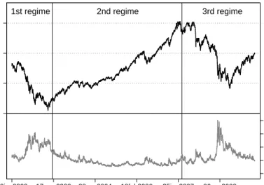
3.2.4. Volatility Regimes . . . 79
3.3. Stylised Empirical Facts of the DAX IVS . . . 82
3.3.1. DAX Volatility Smiles . . . 83
3.3.2. DAX Volatility Term Structures . . . 91
3.3.3. DAX IVS . . . 97
3.3.4. Similarities and Differences between DAX and S&P 500 Index Implied Volatility Before and After Stock Market Crashes . . 100
3.4. Concluding Remarks . . . 103
4. Volatility Forecasting Models 105 4.1. Option Pricing Models . . . 106
4.1.1. Local Volatility Models . . . 106
4.1.2. The Concept of Model-Free Implied Volatility . . . 113
4.1.3. Stochastic Volatility Models . . . 120
4.1.4. Mixed Jump-Diffusion Models and Pure Jump Models . . . . 126
4.2. Time Series Models for Forecasting Volatility . . . 131
4.2.1. GARCH Models . . . 132
5. Forecasting Performance of Volatility Models: A Literature Review 141
5.1. Volatility Forecast Evaluation Based on Encompassing Regressions . . 142
5.1.1. The Definition of Information Efficiency . . . 142
5.1.2. Encompassing Regressions . . . 143
5.2. Empirical Studies Forecasting US Stock Market Volatility . . . 145
5.2.1. The Initial Debate over the Predictive Ability of Implied Volatil-ity . . . 145
5.2.2. The Errors-in-Variables Problem Due to Measurement Errors in Implied Volatility . . . 150
5.2.3. Effects of Using Intraday Returns as an Ex-Post Volatility Measure . . . 152
5.2.4. Implications of the Choice of Option Pricing Model . . . 155
5.2.5. Volatility Forecasts from Long Memory Models . . . 159
5.2.6. Empirical Studies Evaluating Volatility Forecasting Perfor-mance Based on Loss Functions . . . 163
5.2.7. Summary . . . 168
5.3. Empirical Results for the DAX Options Market . . . 171
5.4. Model Selection . . . 178
6. Forecasting DAX Volatility 181 6.1. Data Description . . . 181
6.2. Descriptive Statistics . . . 182
6.3. Tests Results for Unit Roots, Long Memory, and ARCH Effects . . . 186
6.4. Identification, Estimation, and Selection of Volatility Time Series Models . . . 191
6.4.1. GARCH Models . . . 192
6.4.2. ARFIMA and HAR Models . . . 202
6.5. Structural Breaks . . . 204
6.5.1. Testing for Structural Breaks . . . 206
6.5.2. Testing for Long Memory Effects in the Presence of Structural Breaks . . . 208
6.5.3. Testing for Structural Breaks: Results for the HAR model and
the GARCH Models . . . 212
6.6. Volatility Proxy, Evaluation Approach, and Forecasting Methodology 213 6.6.1. Volatility Proxy . . . 214
6.6.2. Forecast Evaluation . . . 219
6.6.3. Forecasting Methodology . . . 232
6.7. Evaluation of the Forecasting Results . . . 233
6.7.1. One-day-ahead Forecasts . . . 235 6.7.2. Two-weeks-ahead Forecasts . . . 241 6.7.3. One-month-ahead Forecasts . . . 246 7. Conclusion 253 A. Appendix of Chapter 3 263 B. Appendix of Chapter 6 265 Bibliography 277
List of Tables
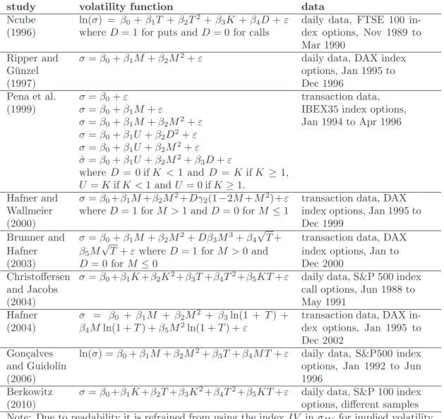
3.1. Studies based on parametric volatility functions . . . 61
6.1. Descriptive statistics of volatility and return series from 2002 to 2009 183 6.2. Correlation matrix . . . 184
6.3. Results of stationarity, long memory, and ARCH LM tests . . . 189
6.4. Estimation results for GARCH models . . . 196
6.5. Diagnostic test results for GARCH models . . . 198
6.6. Estimation results for long memory models . . . 205
6.7. Results of the Bai and Perron (1998) test . . . 210
6.8. Estimation results of the ARFIMA model before and after removing structural breaks . . . 211
6.9. Results of the Andrews (1993) test . . . 213
6.10. MCS results for one-day-ahead forecasts (loss function: MSE) . . . . 237
6.11. MCS results for one-day-ahead forecasts (loss function: QLIKE) . . . 239
6.12. MCS results for two-weeks-ahead forecasts (loss function: MSE) . . . 242
6.13. MCS results for two-weeks-ahead forecasts (loss function: QLIKE) . . 244
6.14. MCS results for one-month-ahead forecasts (loss function: MSE) . . . 247
6.15. MCS results for one-month-ahead forecasts (loss function: QLIKE) . 249 B.1. ADF test results for the null hypothesis “random walk with drift” . . 265
B.2. Information criteria for GARCH model selection . . . 266
B.3. Information criteria for ARFIMA model selection . . . 267
B.5. ADF test results for one-day loss differentials . . . 269 B.6. ADF test results for two-weeks loss differentials . . . 270 B.7. ADF test results for one-month loss differentials . . . 271 B.8. Estimation results for AR(p) processes of one-day loss differentials
(1/2) . . . 272 B.9. Estimation results for AR(p) processes of one-day loss differentials
(2/2) . . . 273 B.10.Estimation results for AR(p) processes of two-weeks loss differentials 274 B.11.Estimation results for AR(p) processes of one-month loss differentials 275
List of Figures
2.1. Types of volatility smiles . . . 19
2.2. Typical S&P 500 post-crash volatility smile . . . 23
2.3. Basic volatility term structure . . . 29
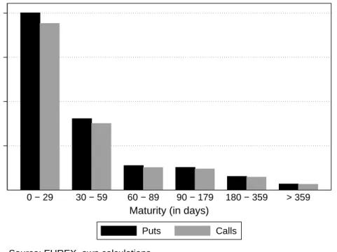
3.1. Transactions of DAX options across maturity from 2002 to 2009 . . . 75
3.2. Transactions of DAX options across moneyness from 2002 to 2009 . . 75
3.3. DAX index level and DAX implied volatilities from 2002 to 2009 . . . 80
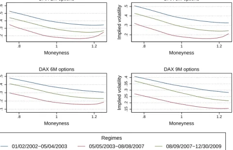
3.4. DAX implied volatility smiles . . . 84
3.5. DAX volatility smiles for different maturities . . . 84
3.6. Average DAX volatility smiles from 2002 to 2009 . . . 86
3.7. Average DAX volatility smiles for different volatility regimes . . . 86
3.8. DAX implied volatilities for different moneyness levels . . . 88
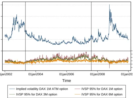
3.9. DAX implied volatility and volatility spreads . . . 88
3.10. DAX implied volatility and volatility spreads for different maturities . 90 3.11. DAX term structures . . . 92
3.12. Average DAX term structures for different moneyness levels . . . 92
3.13. Average DAX term structures for different volatility regimes . . . 94
3.14. DAX implied volatilities for different maturities . . . 94
3.15. DAX implied volatility and volatility term structure spreads . . . 96
3.16. DAX implied volatility and volatility term structure spreads for dif-ferent moneyness levels . . . 96
3.18. Standard deviation of the DAX IVS for the sample period from 2002
to 2009 . . . 98
3.19. Average DAX IVS for the 1st volatility regime . . . 99
3.20. Average DAX IVS for the 2nd volatility regime . . . 99
3.21. Average DAX IVS for the 3rd volatility regime . . . 99
3.22. Time series of DAX implied volatilities . . . 100
6.1. DAX level and DAX return series . . . 185
6.2. DAX volatility series . . . 185
6.3. Correlograms of DAX volatilities and return series . . . 186
6.4. Correlogram of squared DAX return residuals . . . 191
6.5. Correlogram of the DAX return series . . . 193
6.6. p-values for Diebold’s ARCH-robust Q*-statistic . . . 194
6.7. DAX log realised volatility with structural breaks in the mean . . . . 209
A.1. DAX implied volatility surface on May, 2nd 2007. . . 263
A.2. DAX implied volatility surface on October, 16th 2008. . . 263
B.1. Partial autocorrelation function for DAX return series . . . 266
B.2. Correlograms of HAR model residuals . . . 267
List of Abbreviations
AC autocorrelation
ACF autocorrelation function
ADF augmented Dickey-Fuller
AGARCH Asymmetric GARCH
AIC Akaike information criterion
AJD affine jump-diffusion
AR Autoregressive
ARCH Autoregressive Conditional Heteroskedasticity
ARCH LM Autoregressive Conditional Heteroskedasticity Lagrange multiplier
ARFIMA Autoregressive Fractionally Integrated Moving Average
ARIMA Autoregressive Integrated Moving Average
ARMA Autoregressive Moving Average
ATM at-the-money
BS Black-Scholes
BS PDE Black-Scholes partial differential equation
CBOE Chicago Board Options Exchange
CEV constant elasticity of variance
CME Chicago Mercantile Exchange
DAX Deutscher Aktienindex
DFGLS Dickey-Fuller generalised least-squares
DM Diebold-Mariano
DTB Deutsche Terminb¨orse
EGARCH Exponential GARCH
EIV errors-in-variables
EONIA Euro OverNight Index Average
EPA equal predictive ability
EUREX European Exchange
EURIBOR Euro InterBank Offered Rate
EWMA Exponentially Weighted Moving Average
Exc. Kurt. excess kurtosis
FIEGARCH Fractionally Integrated Exponential GARCH
FTSE Financial Times Stock Exchange
GARCH Generalised Autoregressive Conditional Heteroscedasticity
GED generalised error distribution
GJR-GARCH Glosten-Jagannathan-Runkle GARCH
GPH Geweke-Porter-Hudak
HAR Heterogeneous Autoregressive
HMAE mean absolute error adjusted for heteroskedasticity
HMSE mean square error adjusted for heteroskedasticity
HSIC heteroskedastic Schwartz information criterion
IGARCH Integrated GARCH
i.i.d. independent and identically distributed
ITM in-the-money
IVAR integrated variance
IVF implied volatility function
IVS implied volatility surface
IVSP implied volatility spread
IVTSP implied volatility term structure spread
JB Jarque-Bera
KPSS Kwiatkowski-Phillips-Schmidt-Shin
LB Ljung-Box
LHS left hand side
LIFFE London International Financial Futures Exchange
LINEX linear-exponential
LVS local volatility surface
MA Moving Average
MAE mean absolute error
MAPE mean absolute per cent error
MCS model confidence set
ME mean error
MSE mean square error
NASDAQ National Association of Securities Dealers Automated Quations
OTC over-the-counter
OTM out-of-the-money
PACF partial autocorrelation function
PDE partial differential equation
QLIKE quasi-likelihood
QV quadratic variation
RMSE root mean square error
ROB modified version of the GPH test developed by Robinson (1995b)
RV realised variance
RVOLA realised volatility
SD standard deviation
SIC Schwartz information criterion
SOFFEX Swiss Options and Financial Futures Exchange
SPA superior predictive ability
SV stochastic volatility
TAR Threshold Autoregressive
TVSP total volatility spread
VAR Vector Autoregressive
VDAX DAX-Volatilit¨atsindex
VDAX-New DAX-Volatilit¨atsindex New
VIX CBOE Volatility Index
List of Important Symbols
at asset return
A lag polynomial of orderp
b cost-of-carry
B lag polynomial of orderq
C call price
CS cubic spline function
D dummy variable
dq Poisson process
dz Wiener process
E expectation operator
EQ risk-neutral expectation operator
Ft futures price
F∗
t forward price
h bandwidth parameter
ht conditional volatility
h1 bandwidth in the moneyness dimension
h2 bandwidth in the maturity dimension
It−1 information set at time t−1
je expected percentage change in the asset price due to a
Jt independent identically distributed random variable for
the relative change of the asset price in the event of a jump
k average jump size expressed as a percentage of the asset price
K strike price
Kcall
deep−OT M strike price of a deep out-of-the-money option
Kh kernel function
L lag operator
m,mb unknown functional relationship, estimated
M moneyness
n number of observations
N standard normal cumulative distribution function
P put price
pf penalizing function
r risk-free rate
Re real-valued function
S asset price
s2 variance of the jump size
t time
T time to maturity
ut white noise process
U dummy variable
V price of a derivative security
Var variance operator
xt matrix of regressors
ǫ standardised residuals
ζ price of volatility risk
η volatility of volatility
κ rate of mean reversion
λ average number of jumps per unit time
µ drift term π number pi ρ correlation coefficient σ volatility σIV implied volatility τ forecast horizon Ξ Akaike function
1. Introduction
1.1. Motivation and Purpose of the Study
Volatility forecasting plays a key role in financial markets. Investors, risk managers, policy makers, regulators, and researchers need volatility forecasts for investment management, security valuation, risk management, and monetary policy. In the following, volatility is defined as the standard deviation of asset returns.
In the field of investment management, volatility is interpreted as a risk measure and used as an input variable for making investment decisions. In a typical investment process, investors define their risk appetite by the level of risk, or volatility, that they are willing to accept. Then, portfolio managers construct portfolios that take these risk preferences into account. Thus, accurate volatility forecasts enable investors to select investment portfolios, that ideally fit their risk-return profiles.
In addition to asset allocation, volatility forecasting is crucial for option pricing. The on-going growth of the global listed derivatives markets, which in 2013 reached 21.64 billion futures and options contracts, emphasises the importance of this area of appli-cation.1 In modern option pricing theory, beginning with Black and Scholes (1973),
volatility forecasts are directly plugged into the option pricing formula. Moreover, volatility predictions are needed to hedge portfolios of options. Recently, variance
and volatility swaps have been issued, which allow one to directly invest in volatility as an asset class.2
In risk management, the computation of potential portfolio losses, e.g., the value-at-risk, plays a central role. Regulatory authorities, e.g., the European Banking Authority, impose capital requirements that force banks to hold a certain amount of capital to absorb potential future losses. To estimate these potential losses, volatili-ties and correlations have to be predicted. As many risk models failed in the global financial crisis of 2008, practitioners and academics began to revalidate and revise their risk models, including volatility forecasts. Thus, determining the adequacy of volatility predictions, particularly during episodes of turmoil, is crucial for financial institutions.
Further, governments, central banks, and regulatory authorities also monitor finan-cial market volatility. In particular, they consider implied volatility indices that are regarded as market-based measures of economic uncertainty because studies indi-cate that volatility can negatively affect the real economy.3 For example, Bloom
(2014) provides evidence that an increase in uncertainty can reduce employment and economic output.4 Moreover, an empirical paper published by Bekaert et al.
(2013) shows that monetary policy affects risk aversion and uncertainty, which both are potentially related to the business cycle.5 For these reasons, policy makers are
interested in the movement of implied volatility indices.
Therefore, a comprehensive overview of volatility prediction models, and a deep understanding of their ability to produce accurate volatility forecasts is an important task in financial market research. This has been subject of a vast number of empirical and theoretical studies over the past few decades.
2The pay-out of a volatility swap is equal to the difference between the actual volatility and the
predefined contract volatility. See Javaheri et al. (2004), p. 589.
3For example, Poon and Granger (2003) refer to the September 11 terrorist attacks and a series of
corporate accounting scandals at the beginning of the 21st century.
4See Bloom (2014), p. 171.
The simplest volatility prediction model is to calculate the standard deviation of returns over some historical period. The historical standard deviation is then used as a volatility forecast. While in the past, historical volatility was often used to predict volatility, it has been increasingly replaced by more sophisticated time series models that are able to capture the so-called stylised facts of volatility.
These stylised facts are well documented in the literature. The following features are common to many univariate financial time series:6
Fat tails. An important finding is that the distribution of financial returns
exhibits fatter tails than the normal distribution.
Volatility clustering. The volatility clustering effect describes the tendency of
financial volatility to cluster. This means that a large (small) price change tends to be followed by another large (small) price change.
Leverage effect. An unexpected price drop increases volatility more than an
unexpected price increase of equal magnitude.
Long memory effect. Financial market volatility is characterised by long-range
dependencies.
Engle (1982) and Bollerslev (1986) developed a new class of volatility models, the Generalised Autoregressive Conditional Heteroscedasticity (GARCH) models that are able to capture the volatility clustering effect. In the basic GARCH model, the conditional variance depends only on own lags and lags of squared innovations. The concept of Engle (1982) and Bollerslev (1986) was extended by Nelson (1991), Glosten et al. (1993), and Zakoian (1994), among others, to model additional empir-ical characteristics of volatility.7 Because standard GARCH models fail to capture
long memory effects of realised volatilities, Granger and Joyeux (1980) and Hosking (1981) suggested Autoregressive Fractionally Integrated Moving Average (ARFIMA)
6See, for example, Brooks (2008), p. 380 and Poon and Granger (2003), p. 482.
processes to parsimoniously model long memory effects.8 In addition to ARFIMA
models, Corsi (2009) suggests a simple AR-type model for realised volatility that is also able to mimic long memory effects.
These time-series models are complemented by implied volatility, which is derived from options prices by applying a particular option pricing model. In this context, implied volatility is interpreted as the market’s expectation of the underlying asset’s volatility over the remaining lifetime of the option.9 This interpretation of implied
volatility as a market’s expectation of future volatility has been criticised because it requires that the assumptions of the applied option pricing model hold.10 While
most early studies used the Black-Scholes (BS) option pricing model to compute implied volatility, alternative models have since been suggested in the literature. In particular, Poteshman (2000), Shu and Zhang (2003), and Chernov (2007) propose stochastic volatility models, whereas Jiang and Tian (2005) recommend model-free implied volatility to forecast US stock market volatility.
However, despite the restrictive and (often) refuted BS assumptions, many studies demonstrate that BS implied volatility provides better volatility forecasts compared with historical volatility models. For example, Poon and Granger (2005) provide a comprehensive literature review and summarise that implied volatility tends to be more appropriate for predicting volatility than historical volatility models, includ-ing GARCH models.11 Thus, some empirical studies show that BS implied volatility
provides superior forecasting results, although its model assumptions are violated. In this case, the above-cited theoretical foundation for the use of implied volatility to forecast stock market volatility can no longer be maintained, and the predic-tion of financial volatility based on BS implied volatility is nothing more than the application of a heuristic rule.
8Realised volatility is an ex-post measure for return variation in lieu of the true integrated volatility
(see Andersen et al. (2011), p. 221). A detailed definition of realised volatility is given in Section 6.6.1.
9See Canina and Figlewski (1993), Mayhew (1995), and Poon and Granger (2003), among many
others.
10Campbell et al. (1997) note that if the option pricing model does not hold, then the computed
implied volatilities are difficult to interpret. See Campbell et al. (1997), p. 378.
Besides the development and application of more suitable option pricing models, pa-pers by Martens and Zein (2004) and Becker et al. (2006) report that long memory models using realised volatility provide good volatility forecasts that can improve implied volatility forecasts by incorporating incremental information. As a conse-quence, they suggest combined volatility forecasts based on implied volatility and long memory models. Koopman et al. (2005) and Martin et al. (2009) find that long memory models occasionally provide even better prediction results than historical volatility models. In accordance with Martens and Zein (2004), and Becker et al. (2006), they suggest that a combination of individual volatility forecasts from dif-ferent prediction approaches can improve the performance of volatility forecasts.
In addition to extending the set of forecasting models, studies published by Becker and Clements (2008), Martin et al. (2009), and Martens et al. (2009) use more so-phisticated forecast evaluation approaches. Because encompassing regressions only consider individual forecast comparisons, this evaluation approach neglects the com-parison of individual forecasts with the complete set of alternative forecasts.12 By
employing the superior predictive ability (SPA) test suggested by Hansen (2005), or the model confidence set (MCS) approach proposed by Hansen et al. (2003), which both allow for a simultaneous comparison of multiple forecasts, the forecast evalua-tion results of the above studies are not affected by data snooping effects13.14
For the German stock market, the literature presents evidence that DAX implied volatility contains useful information for the prediction of DAX volatility. While Raunig (2006) reports mixed results regarding the relative forecasting performance, recent studies by Muzzioli (2010) and Tallau (2011) suggest that DAX implied volatility provides better volatility forecasts than time series models based on
histor-12See Becker et al. (2007), p. 2536.
13White (2000) describes data snooping as follows (see White (2000), p. 1097):
Data snooping occurs when a given set of data is used more than once for purposes of inference or model selection. When such data reuse occurs, there is always the possibility that any satisfactory results obtained may simply be due to chance rather than to any merit inherent in the method yielding the results.
ical returns. Further, Claessen and Mittnik (2002) indicate that combined volatility forecasts using the information from implied volatility and historical returns are a reasonable complement to individual forecasts. In addition, Lazarov (2004) presents the interesting result that the forecasting performance of ARFIMA models is similar to that of DAX implied volatility. In summary, all these studies of the German stock market examine a subset of forecasting models, but do not provide a comprehen-sive comparison of volatility prediction models. Further, because the above studies concerning the performance of DAX volatility prediction models employ encompass-ing regressions, this is to my knowledge the first study to evaluate DAX volatility forecasts based on the MCS method and DAX realised volatility.15
While a variety of extensive studies on the forecasting performance of implied volatil-ity computed from various option pricing models, time series models, and combina-tions thereof have been published for the US stock market, a similar study for the German stock market that considers all these forecasting models does not exist. In addition, a forecast evaluation approach that controls for data snooping effects has not been applied to compare the prediction results of these models for the German stock market. The intent of this study is to close these research gaps and to provide information to investment and risk managers regarding which forecasting method delivers superior DAX volatility forecasts.
The empirical analysis is based on data that contain all recorded transactions of DAX options and DAX futures traded on the EUREX from January 2002 to De-cember 2009. To select an appropriate time series model for the prediction of DAX volatility, the time series features of DAX returns and realised volatilities are in-vestigated in this thesis. Further, this study presents a detailed analysis of the characteristics of the DAX implied volatility surface (IVS) because the results will provide information for selecting an adequate option pricing model. In particular, the DAX IVS is investigated for three different subsamples because different
volatil-15Further, the MCS approach allows to select the best forecasting models from a range of models,
and it is not necessary to define any specific benchmark model to determine the MCS. Addition-ally, predictions can be compared based on different loss functions.
ity regimes occurred during the sample period. If the DAX IVS exhibits certain regularities during silent and/or turbulent market periods, the selected option pric-ing model should be flexible enough to capture these effects. To my knowledge, this is the first comprehensive analysis of the impact of the financial crisis of 2008 on the DAX IVS.
Due to the discrepancies between the observed patterns of the DAX IVS and the assumptions of the BS model, which provide evidence against the suitability of the BS model for pricing DAX options, the methodologies of alternative option pricing models are presented. In addition, given the time series features of the DAX returns and realised volatilities documented by this study, the methodology of appropriate time series models is described.
After the introduction of the theory underlying the forecasting approaches, a lit-erature review presents the empirical results of selected studies that compare these approaches’ forecasting performance for the US stock market. As such a broad and deep discussion does not exist for the German stock market, the findings of these papers provide useful information for the empirical analysis performed for German stock market volatility.
The volatility prediction models employed in this study to forecast DAX volatility are selected based on the results of these empirical studies, the general features of the forecasting models, and the analysis of the considered DAX time series. Within the class of time series models, the GARCH, the Exponential GARCH (EGARCH), the ARFIMA, and the Heterogeneous Autoregressive (HAR) model are chosen to fit the DAX return and realised volatility series. Additionally, the Britten-Jones and Neuberger (2000) approach is applied to produce DAX implied volatility forecasts because it is based on a broader information set than the BS model. Moreover, recent studies report promising empirical results with respect to the forecasting performance of this approach. Finally, the BS model is employed as a benchmark model in this study.
As the empirical analysis in this study demonstrates that DAX volatility changes considerably over the long sample period, it investigates whether structural breaks induce long memory effects. The effects are separately analysed by performing dif-ferent structural break tests for the prediction models. A discussion of the impact on the applied forecasting methodology, and how it is accounted for, is also presented. Based on the MCS approach, the DAX volatility forecasts are separately evaluated for the full sample and the subperiod that excludes the two most volatile months of the financial crisis. Because the objective of this work is to provide information to investment and risk managers regarding which forecasting method delivers superior DAX volatility forecasts, the volatilities are predicted for one day, two weeks, and one month. Finally, the evaluation results are compared with previous findings in the literature for each forecast horizon.
Overall, this study provides a comprehensive comparison of different forecasting approaches for the German stock market, which yet does not exist. Additionally, this thesis presents the first application of the MCS approach to evaluate DAX volatility forecasts based on high-frequency data. Furthermore, the effects of the 2008 financial crisis on the prediction of DAX volatility, that are not considered in the literature, are analysed.
1.2. Overview of the Thesis
After defining the purpose of the study, Chapter 2 outlines the basic concept of using implied volatilities to predict volatility. Because the BS option pricing model is considered a cornerstone in the history of pricing contingent claims and is often applied as a reference model in empirical studies, it is introduced in this Chapter. Subsequently, a critical review of the use of BS implied volatilities as volatility fore-casts is presented. Further, some stylised facts of BS implied volatilities documented in the literature are described. Finally, selected potential explanatory approaches for the observed BS implied volatility patterns are discussed.
Having presented the pricing biases of the BS model that are documented in the lit-erature, the aim of Chapter 3 is to investigate the (mis)pricing behaviour of the BS model for the German stock market. In particular, this study considers DAX options traded on the EUREX from January 2002 to December 2009. To analyse BS implied volatilities across moneyness and maturity, it is necessary to construct a smooth IVS. Thus, the basic concepts of two general smoothing approaches are discussed, and the choice of the approach employed in this study is explained. Thereafter, the charac-teristics of the DAX BS IVS are described and compared to the existing literature. Moreover, Chapter 3 presents the underlying data set and its preparation.
Because the empirical analysis of the DAX BS IVS demonstrates that some of the BS model assumptions are violated, a range of alternative option pricing models is presented in Chapter 4. To capture the stylised features of the IVS, these models relax some of the BS assumptions. In addition to stochastic volatility and mixed jump-diffusion models, the concept of model-free implied volatility developed by Britten-Jones and Neuberger (2000) is presented. The introduction of this concept is completed by a critical review that considers some additional assumptions necessary for its implementation. The ability of each model class to reproduce the observed DAX IVS is discussed at the end of each Section. In addition to the option pricing models, selected time series models are described that are used in this study to predict DAX volatility.
Chapter 5 presents a literature review of empirical studies comparing the volatility forecasting performance of implied volatility and time series models. Because most early studies use encompassing regressions to evaluate volatility forecasts, the first Section of Chapter 5 introduces this evaluation method. The second Section reviews selected papers on predicting US stock market volatility, as these articles contain broad and intensive discussions of the US stock market. The following Section intro-duces empirical studies on the predictive ability of implied volatility and time series models for German stock market volatility. The final Section explains the choice of the volatility prediction models used in this study to forecast DAX volatility.
Chapter 6 focuses on the generation and evaluation of the DAX volatility forecasts. Due to the characteristics of the DAX return and volatility series, the GARCH, the EGARCH, the ARFIMA, and the HAR models are estimated. Then, information criteria are used to select the most appropriate models. Subsequently, the effects of structural breaks on long memory effects are analysed. Afterwards Section 6.6 explains the choice of the employed volatility proxy, realised volatility, and describes its calculation for the DAX return series. Further, this Chapter contains a brief overview of forecast evaluation techniques and arguments for the selection of the MCS approach applied in this thesis. In the following, the DAX volatility predictions based on the above models are presented for different forecast horizons. In addition to the individual forecasts, this study also considers combined forecasts because some forecast combinations have been found to outperform individual forecasts. Finally, the prediction results are evaluated by using the MCS approach and compared with the previous findings in the literature.
The final Chapter summarises the results, provides recommendations for predict-ing German stock market volatility, and presents an outlook on future research, including possible extensions of this thesis.
2. The Concept of Implied Volatility
Two approaches for predicting financial volatility have been suggested in the litera-ture. The first of these involves the generation of volatility forecasts based on time series models. In the second approach, implied volatilities, which are derived from option prices, can be used to forecast financial volatility.1 First, this Chapter out-lines the basic concept of using implied volatilities to predict volatility.2 Next, the
BS option pricing model is introduced3, which is applied in this study to calculate
implied volatilities from DAX option prices. Finally, the stylised facts of implied volatilities that have been documented in the literature are presented and several corresponding explanatory approaches are discussed.
2.1. The Basic Concept of Using Implied Volatilities
to Forecast Volatility
An option is a derivative security, the price of which depends on the future devel-opment of the underlying asset price. Therefore, option pricing models generally specify a stochastic process to model the price of the underlying asset. Asset volatil-ity is typically one of the main parameters in this process. To compute an option price based on an option pricing model, the volatility parameter has to estimated and plugged into an option pricing formula. Conversely, using an option pricing
1See Poon and Granger (2003), p. 482.
2See Chapter 4 for an introduction to time series models.
model, e.g., the BS model, volatility can also be deduced from the option price. This volatility is called implied volatility.4
Implied volatility is widely interpreted as a market’s expectation of the underlying asset’s volatility over the remaining lifetime of the option, as it is derived from the market price.5 Thus, it is regarded as a “forward-looking” volatility estimate of the
return on the underlying asset,6 which should provide the market’s best volatility
forecast over the option’s maturity.7 Moreover, under the assumption of market
efficiency, implied volatility should provide an informationally efficient forecast of volatility that also contains information on the historical returns of the underlying asset.8,9
Latan´e and Rendleman (1976) provide the first study on the forecasting ability of implied volatilities. They investigate individual stock options traded on the Chicago Board Options Exchange (CBOE) in 1974 and report that a weighted average of implied volatilities is a better predictor of volatility than the standard deviation based on historical returns.10 Although numerous articles have been published on
the forecasting performance of implied volatilities and time series models, the debate over which approach delivers better volatility forecasts persists. A comprehensive literature overview of this discussion is provided in Chapter 6.
However, Campbell et al. (1997) criticise the interpretation of implied volatility as a market’s expectation of future volatility. They argue that implied volatility, which is calculated based on a specific option pricing model, is inseparably related to the model-implicit dynamics of the underlying asset price. Thus, interpreting implied volatility as a market’s prediction of future volatility requires that the option pricing model holds. If the option pricing model does not hold, then the computed implied
4See Rouah and Vainberg (2007), p. 322.
5See Canina and Figlewski (1993), Mayhew (1995), and Poon and Granger (2003) among others.
6See Rouah and Vainberg (2007), p. 304.
7See Ederington and Guan (2005), p. 1429.
8See for example Christensen and Prabhala (1998).
9The literature on the informational content of option prices is discussed in Chapter 5.
volatilities are difficult to interpret.11 Thus, predictive ability tests evaluating
im-plied volatility forecasts are joint tests of predictive ability and the apim-plied option pricing model.12
However, as many studies have demonstrated that implied volatilities exhibit su-perior predictive ability for various options markets, this study investigates their forecasting performance. To account for the argument advanced by Campbell et al. (1997), two different approaches are used to derive implied volatility from option prices. In particular, the approach developed by Britten-Jones and Neuberger (2000) is used to calculate mode-free implied volatility, which does not require the specifi-cation of a particular process for the price of the underlying asset.13 Nonetheless,
the above critique must be kept in mind when the results of the predictive ability tests for implied volatilities are discussed. In the following the most popular option pricing model is presented, namely the BS model, which is used in this study to calculate implied volatilities from option prices.
2.2. The Black-Scholes Model
The development of the BS option pricing model by Black and Scholes (1973) and further by Merton (1973) marks a breakthrough in financial theory. They show that under certain conditions, markets are complete and contingent claim valuation is preference-free. As different studies demonstrate that its assumptions are rather restrictive, the model has been extended in the subsequent literature, and there are currently a large number of refined models available.14 Despite the extensions, the
BS model is considered a cornerstone of pricing contingent claims and is used as a reference model in empirical studies.15 For this reason, the Black-Scholes
par-11See Campbell et al. (1997), p. 378.
12See Jiang and Tian (2005), p. 1306.
13Alternatively, they derive a condition that characterises all continuous price processes that are
consistent with current option prices. See Britten-Jones and Neuberger (2000), p. 839.
14See Fengler (2004), p. 9.
tial differential equation (BS PDE), which under certain assumptions describes the option’s equilibrium price path is derived in the following. The BS option pricing formula is presented on the BS PDE.
To develop the BS option pricing model, Black and Scholes (1973) rely on several assumptions. First, they assume that market participants can trade continuously in a frictionless market where no arbitrage possibilities exist.16 Further, the
under-lying asset pays no dividends, assets are divisible, and short selling is allowed. In addition, investors can lend or borrow without restrictions at the same riskless rate of interest. Moreover, the risk-free interest rate is known and constant over time. While some of the assumptions are not necessary to derive the option pricing model, the following assumption regarding the dynamics of the asset price is essential.17
Black and Scholes (1973) assume that the asset price follows a geometric Brownian motion
dS =µSdt+σSdz (2.1)
where S denotes the underlying asset price,µ the instantaneous drift,σ the instan-taneous volatility, and dz a Wiener process.18
Suppose that V represents the price of an option or other derivative security, the price of which exclusively depends on S and time t. From Itˆo’s lemma, it follows that V can be written as
dV = ∂V ∂SµS+ ∂V ∂t + 1 2 ∂2V ∂S2σ 2S2 dt+ ∂V ∂SσSdz. (2.2)
For a brief time interval ∆t the discrete versions of (2.1) and (2.2) are given by19
∆S =µS∆t+σS∆z (2.3)
16In a frictionless market no transaction costs and or taxes exist.
17Black and Scholes (1973) formulate certain assumptions for expositional convenience.
18See ibid., p. 640.
and ∆V = ∂V ∂SµS + ∂V ∂t + 1 2 ∂2V ∂S2σ 2S2 ∆t+∂V ∂SσS∆z. (2.4)
Based on the underlying asset and the derivative, a portfolio with the value
Π =−V +∂V
∂SS (2.5)
is constructed.20 In a brief time interval ∆t, the portfolio value changes by
∆Π = −∆V + ∂V
∂S∆S. (2.6)
Replacing ∆V and ∆S in (2.6) with (2.3) and (2.4) yields:21
∆Π = −∂V ∂t ∆t− 1 2 ∂2V ∂S2σ 2S2∆t. (2.7)
Because the Wiener processes in (2.3) and (2.4) are identical, they are eliminated in (2.7). It follows that the portfolio in the time interval ∆t is riskless. Thus, the portfolio return must be equal to the risk-free rate, which can be expressed by
∆Π = Πr∆t (2.8)
where r is the risk-free rate.22 It should be noted that the portfolio is only riskless
over an infinitesimal time interval. To ensure that the portfolio is riskless over time, a dynamic hedging strategy is necessary (e.g., delta hedging).23
Substituting equations (2.5) and (2.7) into (2.8) yields the BS PDE
∂V ∂t +rS ∂V ∂S + 1 2σ 2S2∂2V ∂S2 =rV. (2.9)
20The portfolio consists of a short position in the derivative and a long position in the amount of
∂V /∂Sin the underlying asset.
21See Wilmott et al. (1993), p. 43.
22Otherwise riskless arbitrage opportunities would exist which is ruled out by the above
assump-tions. See Wilmott et al. (1993), pp. 43-44.
Under the above assumptions the price of any derivative security must satisfy the BS PDE.24 The solution of the BS PDE depends on the considered derivative which
is specified by its boundary conditions. For instance, for a European call option the boundary condition is
V = max(S−K,0) when t =T (2.10)
where K represents the strike price and T the time to maturity. Based on this final condition, a unique solution for the BS PDE can be derived.25 In the following
the solution of the BS PDE for a European call option is presented. For a detailed derivation see, for instance, Ekstrand (2011).
The solution of the BS PDE for a European call option, which is also called the BS
formula is given by C(S, t) =SN(d1)−Ke−r(T−t)N(d2) (2.11) with d1 = ln(S/K) + (r+σ2/2)(T −t) σ√T −t (2.12) d2= ln(S/K) + (r−σ2/2)(T −t) σ√T −t =d1−σ √ T −t (2.13) where C(·) denotes the price of a European call option and N(·) is the standard normal cumulative distribution function.26 The price of a European put optionP(·)
can be calculated based on the put-call parity by27
P(S, t) =C(S, t) +Ke−r(T−t)−S. (2.14)
24See Wilmott et al. (1993), p. 44.
25See Joshi (2003), p. 105.
26See Wilmott et al. (1993), p. 49.
The assumptions of the BS model have been intensively criticised in the literature.28
In practice, a frictionless market does not exist, a continuous hedge without trans-action costs is impossible, and the asset price does not follow a geometric Brownian motion. Deviations from these assumptions affect the option price and therefore the implied volatility. Thus, whether and in particular to what extent these viola-tions of the BS assumpviola-tions occur can be investigated based on implied volatilities. For this reason, the next Section presents the methodology for deriving BS implied volatilities from option prices.
2.3. Calculation Methodology of Black-Scholes
Implied Volatilities
According to the BS formula, the option price depends on the current time, the level and volatility of the underlying asset price, the interest rate, the strike price, and the maturity date. Except for volatility, all parameters are determined by the contract specification or can be directly observed in the market. As these parameters are fixed, the BS formula defines a one-to-one relationship between the option price and volatility. This, the volatility implied by the market price can be determined by the inverse of the BS formula.29
Formally, given an observed market price Vobs(K, T) of an European option with
strike price K and time to maturity T, the BS implied volatility σIV is defined as
the value of volatility in the BS formula for which the BS option price VBS is equal
to the market price:30
Vobs(K, T) =VBS(σIV, K, T). (2.15)
28See, for instance, Gourieroux and Jasiak (2001a), pp. 321-323, Musiela and Rutkowski (2005),
p. 113, and Chriss (1997), pp. 200-204.
29See Ekstrand (2011), p. 30.
The existence of a unique solution is ensured, as the BS formula is monotonically increasing in volatility.31
The implied volatility cannot be extracted from the BS formula analytically.32
In-stead, it can be computed numerically by finding the root of the objective function
f(σ) =VBS(σ, K, T)−Vobs(K, T) (2.16)
such that f(σIV) = 0.33 The optimisation problem can be solved for instance by
the Newton-Raphson method or the bisection method. It is well known that the Newton-Raphson algorithm is quite sensitive to the initial volatility value, which can lead to unfavourable solutions.34 Further, it requires that the derivative of
the option price with respect to the volatility parameter (vega) is known or can be approximated numerically. In contrast, the bisection method avoids the need for knowledge of vega, as it is based on a simple interpolation method.35 Due to
the Intermediate Value Theorem, the algorithm always finds one root of the above objective function for volatility intervals in which the objective function changes its sign.36 A disadvantage of the bisection method is that it is not as fast as the
Newton-Raphson method. As the Newton-Raphson algorithm can diverge from the root and the speed of the bisection algorithm for the computation of DAX implied volatilities is acceptable, this study employs the bisection algorithm to find the roots of the above objective function.37
While, in theory, the BS implied volatilities of all options on the same underly-ing asset should be identical, in practice, they are not. It is well documented in
31See Cont and da Fonseca (2002), p. 47.
32For the special case of at-the-money (ATM) options, Brenner and Subrahmanyan (1988)
demon-strated that implied volatility can be calculated by a simple approximation formula derived from the BS model.
33See Rouah and Vainberg (2007), p. 305.
34See ibid., p. 307.
35See Haug (2007), p. 455.
36See Rouah and Vainberg (2007), p. 9.
37To assess the effect of the selected algorithm on the resulting implied volatilities, the DAX implied
volatilities are calculated for a subsample based on both algorithms. The results indicated that the differences between the implied volatilities obtained by the Newton-Raphson and the bisection algorithm are very small.
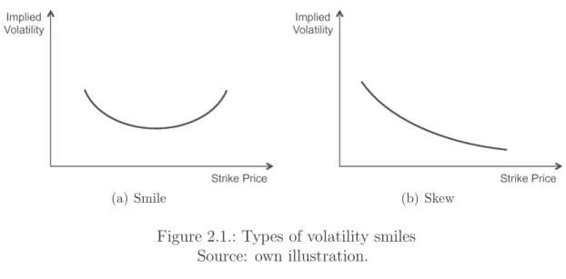
the literature that BS implied volatilities are not constant across strike prices and maturities. Rather, for many options markets, systematic patterns of BS implied volatilities across strike prices and across maturities have been observed. The plot of implied volatilities of options with the same maturity but different strike prices (or moneyness levels) is typically U-shaped. This well-known phenomenon is referred to as the volatility smile. If the shape of the volatility smile is asymmetric, it is called
volatility skew. Figure 2.1 depicts two types of volatility smiles. The functional
relationship between implied volatility and strike price/moneyness is also called the implied volatility function (IVF).38
(a) Smile (b) Skew
Figure 2.1.: Types of volatility smiles Source: own illustration.
Alternatively, if the implied volatilities of options of the same strike price (or mon-eyness level) but different maturities are considered, the implied volatility moves with increasing maturity towards long-term implied volatility. This is called the
volatility term structure.39 The combined analysis of the relationship between
im-plied volatilities and strike prices (volatility smile) and maturities (volatility term structure) is based on the so-called implied volatility surface (or volatility surface).
38The termvolatility smile is synonymously used for the implied volatility function and its plot.
An IVS depicts the implied volatilities for different strike prices and maturities.40
The BS IVS41 at timet is defined as
σiv : (t, K, T)→σiv(K, T). (2.17)
Thus, when the IVS can be fully identified at timet, this means that all (vanilla) call and put option prices are known att.42 Before presenting findings from the empirical
literature on the volatility smile and term structure, the next Section discusses the use of implied volatilities as volatility forecasts.
2.4. A Critical Review of Using Implied Volatilities as
Volatility Forecasts
The interpretation of BS implied volatility as the market’s expectation of the (con-stant) volatility of the underlying asset over the lifetime of the option is based on the validity of the BS model. In particular, the BS model has been criticised for its unrealistic assumption of constant volatility.43 Feinstein (1989) shows that this
assumption can be relaxed. He demonstrates that the BS implied volatility from a near-expiration ATM call option yields an unbiased forecast of the average volatility over the remaining life of the option when volatility is stochastic and uncorrelated with aggregate consumption.44 The assumption of zero correlation between volatility
changes and aggregate consumption changes ensures that volatility risk is unpriced in the market. However, the empirical results of Lamoureux and Lastrapes (1993) call this assumption into question, as they report that the market price of volatility risk for individual US stocks is nonzero and time varying. Thus, Feinstein’ s (1989) finding cannot be used as a general argument in favour of the BS model. For this
40See Hull (2006), p. 382.
41The termvolatility surface is used for the preceding function and its graphical representation.
42See Cont and da Fonseca (2002), p. 45.
43See, for instance, Gourieroux and Jasiak (2001a), p. 279.
44The Hull and White (1987) option pricing model provides the theoretical framework for this
reason, advanced option pricing models, e.g., the stochastic volatility model sug-gested by Heston (1993), have been developed to take time-varying volatility into account.
Despite the unrealistic assumptions of the BS model and the availability of stochas-tic volatility models, option traders typically quote prices in terms of BS implied volatilities. By expressing option prices as BS implied volatilities, traders seek to control for different strike prices and maturities.45 Campbell et al. (1997) argue
that this only reflects the popularity of the BS formula as a heuristic, but has no economic implications. Further, they note that option traders quoting prices using BS implied volatilities does not necessarily imply that they calculate their prices based on the BS formula. They conclude that due to the one-to-one relationship between BS implied volatilities and option prices, both pricing measures cover the same information.46 Thus, if the BS model does not hold, the use of BS implied
volatilities as volatility forecasts corresponds to the application of a heuristic rule. However, even if one agrees with this interpretation of BS implied volatility, it is an interesting research topic to compare its forecasting ability with those of alternative prediction approaches. The next Section reports some well-known stylised facts of implied volatilities, including the volatility smile and the volatility term structure, which have been documented in the literature.
2.5. Stylised Facts of Implied Volatilities
This Section begins with a review of the discussion on the volatility smile effect. The discussion covers two basic forms of the volatility smile and presents some important empirical results for different options markets. Subsequently, the term structure of implied volatility is described. Finally, the time series properties of implied volatilities that have been observed for some selected options markets are presented.
45See Hafner (2004), p. 37.
2.5.1. The Smile Effect
From Smiles and SkewsThe first two articles documenting the systematic pattern of BS pricing errors across strike prices and maturities are Black (1975) and MacBeth and Merville (1979). Using CBOE prices for the period from 1973 to 1975, Black (1975) reports that the actual market prices of out-of-the-money (in-the-money) options tend to be higher (lower) than the values given by the BS formula. He suggests different explanations for this pattern including time-varying volatility, tax factors, speculative profits, and leverage restrictions.47 In contrast, MacBeth and Merville (1979) find that
implied volatilities of CBOE options tend to increase with decreasing strike prices for the period from 1975 to 1976. Rubinstein (1985) analyses trades and quotes on the 30 most active option classes for individual stocks in the CBOE from August 1976 to August 1978 and finds that the implied volatilities of short-term out-of-the-money (OTM) calls are higher than for other calls.48 By considering different
time periods, he demonstrates that the sign of the price differences between market prices and BS values changes over time. However, he notes that while the option price differences are indeed statistically significant, their economic significance is questionable.49 Moreover, Mixon (2009), who investigates empirical regularities of
implied volatilities in the 19th century and the 21st century, provides early evidence in favour of the existence of an implied volatility skew in the 19th century.50 Thus,
the findings of Black (1975), Rubinstein (1985), Mixon (2009), and others show that the volatility smile phenomenon already existed at least in a weak form in some options markets before the stock market crash in 1987, which marks a decisive turning point for volatility smiles.51
47See Black (1975), pp. 64-65.
48See Rubinstein (1985), p. 474.
49See ibid., p. 478.
50See Mixon (2009), p. 172.
51The dramatic decline in the stock market on October 19th and 20th, 1987 of more than 20% was
the greatest decline since 1929. The crash of 1987 was preceded by an extraordinary increase of 42% in 1987.
.14 .16 .18 .2 .22 .24 Implied volatility .85 .9 .95 1 1.05 1.1 Moneyness
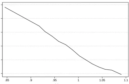
Source: See Rubinstein (1994), p. 776. Note: Implied volatilities based on S&P 500 index options from January 2nd, 1990 at 10:00 a.m.
Figure 2.2.: Typical S&P 500 post-crash volatility smile
Prior the crash of 1987, implied volatilities in stock options markets typically formed a symmetric smile pattern when plotted against strike price or moneyness. After the crash of 1987, the shape of implied volatilities for most stock index options mar-kets more resembles a skew, where implied volatilities decrease monotonically as the strike price rises.52,53 Figure 2.2 depicts a typical downward sloping post-crash smile
for S&P 500 index options. The change in the form of the volatility smile towards a skew shape implies that after the crash of 1987, market participants have paid higher prices for OTM put and in-the-money (ITM) call options relative to other options. Rubinstein (1994) argues that the overpricing of put options is induced by an excess demand for put options, which provide portfolio insurance against market downturns. The excess demand for put options reflects investors’ concerns regarding another stock market crash. Rubinstein (1994) terms this phenomenon “crash-o-phobia”.54 The volatility skew phenomenon did not disappear following the
crash. This also implies that the implicit distribution of option prices has shifted
52See, for example, Poon and Granger (2003), p. 487 and Cont and Tankov (2004), p. 10.
53In addition to this permanent effect, implied volatility remained at a high level for several months
after the crash (implied volatility more than doubled), but had returned to a pre-crash level by March 1988.
from a widely symmetric and positively skewed distribution to a substantially neg-atively skewed distribution.55 As Rubinstein (1994) highlights, the crash of 1987
permanently changed market participants’ perceptions and pricing mechanisms for stock index options. For this reason, in the next Chapter, this study also investigates whether the 2008 financial crisis affects the volatility smile of DAX options. The following Section provides an overview of the empirical results concerning volatility smiles across different options markets.
Empirical Evidence for Volatility Smiles Across Different Options Markets
The volatility smile effect has been observed for many options markets.56 Analysing
daily over-the-counter (OTC) implied volatility quotes on 12 major equity indices (i.e., CAC (France), DAX (Germany), FTSE (United Kingdom), HSI (Hong Kong), NKY (Japan), and SPX (United States)) from June 1995 to May 2005, Foresi and Wu (2005) confirm the existence of a heavily skewed implied volatility pattern for all indices examined. Interestingly, they find that the markets differ more in the level of implied volatility than in the skewness of the volatility smile. Overall, they conclude that the volatility skew is not a local observation, but rather a worldwide phenomenon.57
In a broad study, Tompkins (2001) considers 16 options markets with respect to stock indices, bonds, exchange rates, and forward deposits over long time periods and compares the regularities of the IVS across the different markets. His sample comprises, for most markets, option closing prices over ten years beginning in the mid-1980s and ending in the mid-1990s.58 Overall, he finds that the shapes of the implied volatilities, which are smoothed based on a quadratic regression, exhibit
55See Bates (2000), p. 182.
56For a comprehensive overview of stock, bond and exchange rate markets, see, e.g., Rebonato
(2004).
57See Foresi and Wu (2005), pp. 11-13.
58To avoid the problem of non-synchronous trading, Tompkins (2001) only examines OTM put
and call options with maturities up to 90 days. To control for level effects, which according to Dumas et al. (1998) contain no exploitable information on future levels of implied volatility, he uses standardised implied volatilities.
similar patterns for options within the same asset class. First, the smoothed implied volatilities of short-term stock options on the S&P 500, the FTSE, the Nikkei, and the DAX index are “U-shaped” across moneyness. Second, the volatility smiles for options with 90 days to maturity generally exhibit a comparatively linear skewed form.59 Moreover, the regression results support the findings of Rubinstein (1994)
and others that the negative volatility skew of S&P 500 options is related to the 1987 stock market crash. However, he reports that a second shock in 1989 also contributes to the negative skewness of the S&P 500 volatility smile.60 Furthermore, he mentions
that the IVS in all considered stock index options markets becomes flatter when the level of implied volatility of ATM options increases in the markets.61
In addition to the above basic facts regarding stock volatility smiles, Rebonato (2004) adds that the smile is generally much more pronounced at short maturities and flattens out at longer maturities. Furthermore, the smile of OTM puts is typ-ically steeper than the smile of OTM calls. In some cases, the smile completely disappears for OTM calls. Moreover, during periods of high volatility, Rebonato (2004) notes that the asymmetry of the smile usually tends to increase.62 Next, the
empirical results concerning the volatility smile for the German options market are presented.
Empirical Studies of the DAX Volatility Smile
Few empirical findings regarding the existence of a volatility smile in the German options market before the 1987 crash are provided in the literature. For instance, Trautmann (1990) describes systematic pricing biases in the BS model. He considers pricing differences between market prices and BS values of individual stock options
59Tompkins (2001) reports comparable findings for interest rate options (US Treasury Bonds, UK
Gilts, German Bundesanleihen, and Italian Government Bonds). The volatility smiles of foreign exchange rate options (US Dollar/Deutsche Mark, US Dollar/British Pound, US Dollar/Japanese Yen and US Dollar/Swiss Franc) exhibit the most similarities. See Tompkins (2001), p. 204.
60While both shocks also change the smile of FTSE 100 index options, the DAX volatility smile is
unaffected.
61See Tompkins (2001), pp. 200-218.
traded on the Frankfurter Optionsb¨orse from 1983 to 1987. Based on these data, he demonstrates that the BS model underprices deep OTM call options on individual stocks with maturities beyond four weeks.63 Thus, the results indicate that the
BS assumption of constant volatility had been violated for individual stock options traded on the Frankfurter Optionsb¨orse before the stock market crash of 1987.64
Evidence for the existence of a post-crash DAX volatility smile is reported by Beinert and Trautmann (1995), Ripper and G¨unzel (1997), Herrmann (1999), and Bolek (1999), among others. Beinert and Trautmann (1995) use transaction prices for the most liquid call options on individual stocks traded on the Deutsche Terminb¨orse (DTB) from 1990 to 1991. In particular, they demonstrate the volatility smile of short-term options has a U-shaped form. In summary, they conclude that the smile pattern is typical of options traded on the DTB, but did not hold in every case.65 Ripper and G¨unzel (1997) estimate the IVS based on a regression using
daily settlement prices on DAX options for the years 1995 to 1996 listed on the DTB. The results indicate a volatility smile for short-term options and a skew for long-term options (with maturities beginning at three months).66 Herrmann (1999)
confirms the results of Ripper and G¨unzel (1997) with respect to the existence of a volatility smile for short-term options. His analysis is based on transaction data of DAX options traded on the DTB from 1992 to 1997. Additionally, he finds that the implied volatilities of ITM and OTM options in the same moneyness class typically decline with increasing maturity. In contrast, he reports increasing implied volatilities for ATM options if the time to maturity is extended. Further, the highest implied volatilities are recorded for deep ITM calls and deep ITM puts. Moreover, he reports that DAX puts have higher implied volatilities than DAX calls of the same moneyness/maturity class.67 Bolek’s (1999) study is based on the closing
prices of DAX options traded on the DTB in the 2nd half of 1995. His findings also
63See Trautmann (1990), p. 95.
64As was the case for the US stock market, the DAX declined dramatically in 1987 (approximately
22% from September 1987 to October 1987).
65See Beinert and Trautmann (1995), p. 13.
66See Ripper and G¨unzel (1997), p. 475.
support the existence of a DAX volatility smile, especially for short-term options.68
The minimum of the smile of short-term DAX options is located ATM. For long-term DAX calls, the minimum of the smile is OTM. In this case, the smile nearly disappears. In contrast, the minimum of the DAX volatility smile for long-term put options is ITM and the smile is less pronounced. By plotting the volatility smile implied by DAX calls and puts for successive trading days, he finds evidence that the smile changes over time.69
Subsequently, Tompkins (2001) and Wallmeier (2003) also examine the systematic pattern of DAX implied volatilities.70 Tompkins (2001) analyses DAX option closing
prices for the time period from January 1992 to December 1996. Using the quadratic regression approach suggested by Shimko (1993), he finds that the volatility smile is negatively skewed. Further, the IVF was more skewed for short-term options than for options with longer maturities.71 Wallmeier (2003) investigates transaction
prices of DAX options for the period from 1995 to 2000. His results also reveal the existence of a DAX volatility skew rather than a smile. Moreover, he reports that the magnitude of the skew tends to decrease as the level of ATM implied volatility rises. He concludes that in the sample period, DAX implied volatilities differ considerably across strike prices and maturities. Therefore, he notes that the BS assumption of constant volatility is seriously violated.72
More recent evidence concerning DAX implied volatility smiles is provided by Brun-ner and HafBrun-ner (2003), Fengler et al. (2003), HafBrun-ner (2004), Fengler et al. (2007), Detlefsen (2007), Schnellen (2007), and Br¨uggemann et al. (2008).73 Walter (2008)
considers the volatility smile of individual German stocks. The next Section de-scribes empirical regularities of the volatility term structure
68Bolek (1999) defines short-term options as options with maturities of up to 15 trading days.
69See ibid., pp. 122-128.
70In particular, both studies consider the factors influencing the IVS. The results are presented in
the last Section of this Chapter.
71See Tompkins (2001), p. 204.
72See Wallmeier (2003), pp. 190-208.
2.5.2. The Volatility Term Structure
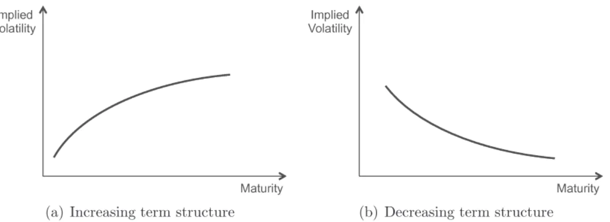
Basic Volatility Term StructuresIn addition to providing extensive evidence of the volatility smile, the term structure of implied volatility is intensively discussed in literature. In Chapter 2.3, the term structure of volatility was defined as the relationship between implied volatility and time to maturity for a given strike price (or moneyness level).74 The constant
volatility assumption of the BS model implies a flat term structure. Therefore, the implied volatilities of short-term and long-ter