Probe, Count, and Classify:
Categorizing Hidden-Web Databases
Panagiotis G. Ipeirotis
Computer Science Dept.
Columbia University
Luis Gravano
Computer Science Dept.
Columbia University
Mehran Sahami
E.piphany, Inc.
ABSTRACT
The contents of many valuable web-accessible databases are only accessible through search interfaces and are hence in-visible to traditional web “crawlers.” Recent studies have estimated the size of this “hidden web” to be 500 billion pages, while the size of the “crawlable” web is only an es-timated two billion pages. Recently, commercial web sites have started to manually organize web-accessible databases into Yahoo!-like hierarchical classification schemes. In this paper, we introduce a method for automating this classi-fication process by using a small number of query probes. To classify a database, our algorithm does not retrieve or in-spect any documents or pages from the database, but rather just exploits the number of matches that each query probe generates at the database in question. We have conducted an extensive experimental evaluation of our technique over collections of real documents, including over one hundred web-accessible databases. Our experiments show that our system has low overhead and achieves high classification ac-curacy across a variety of databases.
1.
INTRODUCTION
As the World-Wide Web continues to grow at an expo-nential rate, the problem of accurate information retrieval in such an environment also continues to escalate. One es-pecially important facet of this problem is the ability to not only retrieve static documents that exist on the web, but also effectively determine which searchable databases are most likely to contain the relevant information that a user is looking for. Indeed, a significant amount of informa-tion on the web cannot be accessed directly through links, but is available only as a response to a dynamically issued query to the search interface of a database. The results page for a query typically contains dynamically generated links to these documents. Traditional search engines cannot handle such interfaces and ignore the contents of these resources, since they only take advantage of the static link structure of the web to “crawl” and index web pages.
The magnitude of the importance of this problem is
high-Permission to make digital or hard copies of all or part of this work for personal or classroom use is granted without fee provided that copies are not made or distributed for profit or commercial advantage and that copies bear this notice and the full citation on the first page. To copy otherwise, to republish, to post on servers or to redistribute to lists, requires prior specific permission and/or a fee.
ACM SIGMOD 2001 May 21-24, Santa Barbara, California, USA
Copyright 2001 ACM 1-58113-332-4/01/05 ...$5.00.
lighted in recent studies [6] that estimated that the amount of information “hidden” behind such query interfaces out-numbers the documents of the “ordinary” web by two orders of magnitude. In particular, the study claims that the size of the “hidden” web is 500 billion pages, compared to “only” two billion pages of the ordinary web. Also the contents of these databases are many times topically cohesive and of higher quality than those of ordinary web pages.
Even sites that have some static links that are “crawlable” by a search engine may have much more information avail-able only through a query interface, as the following real example illustrates.
Example 1.: Consider the PubMed medical database from the National Library of Medicine, which stores medi-cal bibliographic information and links to full-text journals accessible through the web. The query interface is available at http://www.ncbi.nlm.nih.gov/PubMed/. If we query PubMed for documents with the keywordcancer, PubMed returns 1,301,269 matches, corresponding to high-quality ci-tations to medical articles. The abstracts and cici-tations are stored locally at the PubMed site and are not distributed over the web. Unfortunately, the high-quality contents of PubMed are not “crawlable” by traditional search engines. A query1 on AltaVista2that finds the pages in the PubMed site with the keyword “cancer,” returns only 19,893 matches. This number not only is much lower than the number of PubMed matches reported above, but, additionally, the pa-ges returned by AltaVista are links to other web papa-ges on the PubMed site, not toarticles in the PubMed database.
2
For dynamic environments (e.g., sports), querying a text database may be the only way to retrieve fresh articles that are relevant, since such articles are often not indexed by a search engine because they are too new, or because they change too often.
In this paper we concentrate onsearchable web databases of text documents regardless of whether their contents are crawlable or not. More specifically, for our purposes a sea-rchable web database is a collection of text documents that is searchable through a web-accessible search interface. The documents in a searchable web database do not necessar-ily reside on a single centralized site, but can be scattered over several sites. Our focus is on text: 84% of all search-able databases on the web are estimated to provide access to text documents [6]. Other searchable sites offer access to 1
The query iscancer host:www.ncbi.nlm.nih.gov.
other kinds of information (e.g., image databases and shop-ping/auction sites). A discussion on these sites is out of the scope of this paper.
In order to effectively guide users to the appropriate sea-rchable web database, some web sites (described in more detail below) have undertaken the arduous task of manually classifying searchable web databases into a Yahoo!-like hier-archical categorization scheme. While we believe this type of categorization can be immensely helpful to web users trying to find information relevant to a given topic, it is hampered by the lack of scalability inherent in manual classification.
Consequently, in this paper we propose a method for the automatic categorization of searchable web databases into topic hierarchies using a combination of machine learning and database querying techniques. Through the use ofquery probing, we present a novel and efficient way to classify a searchable database without having to retrieve any of the actual documents in the database. We use machine learning techniques to initially build a rule-based classifier that has been trained to “classify” documents that may be hidden behind searchable interfaces. Rather than actually using this classifier to categorize individual documents, we trans-form the rules of the classifier into a set of query probes that can be sent to the search interface for various text databases. Our algorithm can then simply use the counts for the number of documents matching each query to make a classification decision for the topic(s) of the entire database, without having to analyze any of the actual documents in the database. This makes our approach very efficient and scalable.
By providing an efficient automatic means for the accurate classification of searchable text databases into topic hierar-chies, we hope to alleviate the scalability problems of manual database classification, and make it easier for end-users to find the relevant information they are seeking on the web.
The contributions presented in this paper are organized as follows: In Section 2 we more formally define and pro-vide various strategies for database classification. Section 3 presents the details of our query probing algorithm for data-base classification. In Sections 4 and 5 we provide the exper-imental setting and results, respectively, of our classification method and compare it with two existing methods for au-tomatic database classification. The method we present is shown to be both more accurate as well as more efficient on the database classification task. Finally, Section 6 describes related work, and Section 7 provides conclusions and out-lines future research directions.
2.
TEXT-DATABASE CLASSIFICATION
As shown previously, the web hosts many collections of documents whose contents are only accessible through a search interface. In this section we discuss how we can orga-nize the space of such searchable databases in a hierarchical categorization scheme. We first define appropriate classifi-cation schemes for such databases in Section 2.1, and then present alternative methods for text database categorization in Section 2.2.
2.1
Classification Schemes for Databases
Several commercial web directories have recently started tomanuallyclassify searchable web databases, so that users can browse these categories to find the databases of
inter-WNBA CBS Sportsline
- Basket
ESPN Baseball Basketball Volleyball Arts Computers Health Science Sports
Root ... ... ... ... ... ... ... ... ... ...
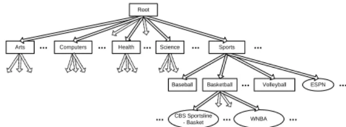
Figure 1: Portion of the InvisibleWeb classification scheme.
est. Examples of such directories include InvisibleWeb3and SearchEngineGuide4. Figure 1 shows a small fraction of In-visibleWeb’s classification scheme.
Formally, we can define a hierarchical classification scheme like the one used by InvisibleWeb as follows:
Definition 1.: Ahierarchical classification scheme is a rooted directed tree whose nodes correspond to (topic) cate-gories and whose edges denote specialization. An edge from categoryvto another categoryv0indicates thatv0is a
sub-category ofv. 2
Given a classification scheme, our goal is to automatically populate it with searchable databases where we assign each database to the “best” category or categories in the scheme. For example, InvisibleWeb has manually assigned WNBA to the“Basketball” category in its classification scheme. In general we can define what category or categories are “best” for a given database in several different ways, according to the needs the classification will serve. We describe different such approaches next.
2.2
Alternative Classification Strategies
We now turn to the central issue of how to automatically assign databases to categories in a classification scheme, as-suming complete knowledge of the contents of these data-bases. Of course, in practice we will not have such complete knowledge, so we will have to use the probing techniques of Section 3 to approximate the “ideal” classification defini-tions that we give next.
To assign a searchable web database to a category or set of categories in a classification scheme, one possibility is to manually inspect the contents of the database and make a decision based on the results of this inspection. Inciden-tally, this is the way in which commercial web directories like InvisibleWeb operate. This approach might produce good quality category assignments, but, of course, is expen-sive (it includes human participation) and does not scale well to the large number of searchable web databases.
Alternatively, we could follow a less manual approach and determine the category of a searchable web database based on the category of the documents it contains. We can for-malize this approach as follows: Consider a web database
D and a number of categories C1, . . . , Cn. If we knew the category Ci of each of the documents inside D, then we could use this information to classify databaseD in at least two different ways. A coverage-based classification will as-sign D to all categories for whichD has sufficiently many documents. In contrast, aspecificity-basedclassification will assign D to the categories that cover a significant fraction ofD’s holdings.
3http://www.invisibleweb.com 4http://www.searchengineguide.com
Example 2.: Consider topic category“Basketball.” CBS SportsLine has a large number of articles about basketball and covers not only women’s basketball but other basket-ball leagues as well. It also covers other sports like footbasket-ball, baseball, and hockey. On the other hand,WNBAonly has articles about women’s basketball. The way that we will classify these sites depends on the use of our classification. Users who prefer to seeonly articles relevant to basketball might prefer aspecificity-based classification and would like to have the site WNBA classified into node “Basketball.” However, these users would not want to have CBS Sport-sLine in this node, since this site has a large number of articles irrelevant to basketball. In contrast, other users might prefer to have only databases with a broad and com-prehensive coverage of basketball in the“Basketball” node. Such users might prefer acoverage-based classification and would like to findCBS SportsLinein the“Basketball”node, which has a large number of articles about basketball, but notWNBAwith only a small fraction of the total number of basketball documents. 2
More formally, we can use the number of documents fi in categoryCi that we find in databaseDto define the fol-lowing two metrics, which we will use to specify the “ideal” classification ofD.
Definition 2.: Consider a web databaseD, a hierarchi-cal classification schemeC, and a categoryCi ∈C. Then thecoverage ofDforCi,Coverage(D, Ci), is the number of documents inDin categoryCi,fi.
Coverage(D, Ci) =fi
IfCkis the parent ofCi inC, then thespecificity ofD for
Ci,Specificity(D, Ci), is the fraction ofCk documents inD that are in categoryCi. More formally, we have:
Specificity(D, Ci) = fi
|Documents in D about Ck| As a special case,Specificity(D,root) = 1. 2
Specificity(D, Ci) gives a measure of how “focused” the data-baseDis on a subcategoryCiofCk. The value ofSpecificity ranges between 0 and 1. Coverage(D, Ci) defines the “abso-lute” amount of information that databaseDcontains about categoryCi5. For notational convenience we define:
Coverage(D)=hCoverage(D, Ci1), . . . ,Coverage(D, Cim)i
Specificity(D)=hSpecificity(D, Ci1), . . . ,Specificity(D, Cim)i
when the set of categories{Ci1, . . . , Cim}is clear from the
context.
Now, we can use the Specificity and Coverage values to decide how to classifyD into one or more categories in the classification scheme. As described above, aspecificity-based classificationwould classify a database into a category when a significant fraction of the documents it contains are of this specific category. Alternatively, acoverage-based clas-sification would classify a database into a category when the database has a substantial number of documents in the given category. In general, however, we are interested in 5It would be possible to normalizeCoveragevalues to be between 0
and 1 by dividingfiwith the total number of documents in category
Ci across all databases. Although intuitively appealing (Coverage would then measure the fraction of the universally available informa-tion aboutCithat is stored inD), this definition is “unstable” since each insertion, deletion, or modification of a web database changes
theCoverageof the other available databases.
balancing bothSpecificity and Coverage through the intro-duction of two associated thresholds,τsandτc, respectively, as captured in the following definition.
Definition 3.: Consider a classification schemeC with categories C1, . . . , Cn, and a searchable web database D. Theideal classification ofD inCis the setIdeal(D)of cat-egoriesCithat satisfy the following conditions:
• Specificity(D, Ci)≥τs.
• Specificity(D, Cj)≥τsfor all ancestorsCjofCi.
• Coverage(D, Ci)≥τc.
• Coverage(D, Cj)≥τc for all ancestorsCjofCi.
• Coverage(D, Ck) < τc orSpecificity(D, Ck) < τs for all childrenCkofCi.
with 0≤τs≤1 andτc≥1 given thresholds. 2
The ideal classification definition given above provides al-ternative approaches for “populating” a hierarchical classi-fication scheme with searchable web databases, depending on the values of the thresholds τs and τc. A low value for the specificity threshold τs will result in a coverage-based classification of the databases. Similarly, a low value for the coverage thresholdτcwill result in a specificity-based classi-fication of the databases. The values of choice forτsandτc are ultimately determined by the intended use and audience of the classification scheme. Next, we introduce a technique for automatically populating a classification scheme accord-ing to the ideal classification of choice.
3.
CLASSIFYING DATABASES THROUGH
PROBING
In the previous section we defined how to classify a data-base data-based on the number of documents that it contains in each category. Unfortunately, databases typically do not export such category-frequency information. In this section we describe how we can approximate this information for a given database without accessing its contents. The whole procedure is divided into two parts: First we train our sys-tem for a given classification scheme and then we probe each database with queries to decide the categories to which it should be assigned. More specifically, we follow the algo-rithm below:
1. Train a rule-based document classifier with a set of preclassified documents (Section 3.1).
2. Transform classifier rules into queries (Section 3.2). 3. Adaptively issue queries to databases, extracting and
adjusting the number of matches for each query using the classifier’s “confusion matrix” (Section 3.3). 4. Classify databases using the adjusted number of query
matches (Section 3.4).
3.1
Training a Document Classifier
Our database classification technique relies on a rule-based document classifier to create the probing queries, so our first step is to train such a classifier. We use supervised learning to construct a rule-based classifier from a set of preclas-sified documents. The resulting classifier is a set of logi-cal rules whose antecedents are conjunctions of words, and whose consequents are the category assignments for each document. For example, the following rules are part of a classifier for the three categories “Sports,” “Health,” and “Computers”:
IF ibm AND computer THEN Computers IF jordan AND bulls THEN Sports IF diabetes THEN Health
IF cancer AND lung THEN Health IF intel THEN Computers
Such rules are used to classify previously unseen docu-ments (i.e., docudocu-ments not in the training set). For exam-ple, the first rule would classify all documents containing the words “ibm” and “computer” into the category “Com-puters.”
Definition 4.: Arule-based document classifierfor aflat set of categoriesC={C1, . . . , Cn}consists of a set of rules
pk→Clk, k= 1, . . . , m, wherepkis a conjunction of words and Clk ∈ C. A document d matches a rule pk → Clk if
all the words in that rule’s antecedent,pk, appear in d. If a documentdmatches multiple rules with different classifi-cation decisions, the final classificlassifi-cation decision depends on the specific implementation of the rule-based classifier. 2
To define a document classifier over an entire hierarchical classification scheme (Definition 1), we train one flat rule-based document classifier for eachinternal node of the hi-erarchy. To produce a rule-based document classifier with a concise set of rules, we follow a sequence of steps, described below.
The first step, which helps both efficiency and effective-ness, is to eliminate from the training set all words that appear very frequently in the training documents, as well as very infrequently appearing words. This initial “feature selection” step is based on Zipf’s law [32]. Very frequent words are usually auxiliary words that bear no information content (e.g., “am”, “and”, “so” in English). Infrequently occurring words are not very helpful for classification either, because they appear in so few documents that there are no significant accuracy gains from including such terms in a classifier.
The elimination of words dictated by Zipf’s law is a form of feature selection. However, frequency information alone is not, after some point, a good indicator to drive the feature selection process further. Thus, we use an information the-oretic feature selection algorithm that eliminates the terms that have the least impact on the class distribution of docu-ments [16, 15]. This step eliminates the features that either do not have enough discriminating power (i.e., words that are not strongly associated with one specific category) or features that are redundant given the presence of another feature. Using this algorithm we decrease the number of features in a principled way and we can use a much smaller subset of words to create the classifier, with minimal loss in accuracy. Additionally, the remaining features are generally more useful for classification purposes, so rules constructed from these features will tend to be more meaningful for gen-eral use.
After selecting the features (i.e., words) that we will use for building the document classifier, we use RIPPER, a tool built at AT&T Research Laboratories [4], to actually learn the classifier rules. Once we have trained a document clas-sifier, we could use it to classify all the documents in a database of interest. We could then classify the database itself according to the number of documents that it contains in each category, as described in Section 2. Of course, this requires having access to the whole contents of the database, which is not a realistic requirement for web databases. We relax this requirement next.
3.2
Defining Query Probes from a Document
Classifier
In this section we show how we can map the classification rules of a document classifier intoquery probes that will help us estimate the number of documents for each category of interest in a searchable web database.
To simulate the behavior of a rule-based classifier over all documents of a database, we map each rule pk → Clk of
the classifier into a boolean queryqkthat is the conjunction of all words inpk. Thus, if we send the query probeqk to the search interface of a database D, the query will match exactly thef(qk) documents in the databaseD that would have been classified by the associated rule into categoryClk. For example, we map the ruleIF jordan AND bulls THEN Sports into the boolean queryjordan AND bulls. We ex-pect this query to retrieve mostly documents in the“Sports” category. Now, instead of retrieving the documents them-selves, we just keep the number of matches reported for this query (it is quite common for a database to start the re-sults page with a line like “X documents found”), and use this number as a measure of how many documents in the database match the condition of this rule.
From the number of matches for each query probe, we can construct a good approximation of the Coverage and Specificity vectors for a database (Section 2). We can ap-proximate the number of documents fj in Cj inD as the total number of matches gj for the Cj query probes. The result approximates the distribution of categories of theD
documents. Using this information we can approximate the Coverage andSpecificity vectors as follows:
Definition 5.: Consider a searchable web database D
and a rule-based classifier for a set of categoriesC. For each query probeqderived from the classifier, databaseDreturns the number of matches f(q). Then theestimated coverage of D for a category Ci ∈C, ECoverage(D,Ci), is the total number of matches for theCiquery probes.
ECoverage(D,Ci) = X
q is a query probe forCi
f(q) Theestimated specificity ofD forCi,ESpecificity(D,Ci), is ESpecificity(D,Ci) = P ECoverage(D,Ci)
q is a query probe for anyCjf(q)
2
For notational convenience we define:
ECoverage(D)=hECoverage(D, Ci1), . . . ,ECoverage(D, Cim)i
ESpecificity(D)=hESpecificity(D, Ci1), . . . ,ESpecificity(D, Cim)i
when the set of categories {Ci1, . . . , Cim} is clear from the
context.
Example 3.: Consider a small rule-based document clas-sifier for categories C1=“Sports,” C2=“Computers,” and
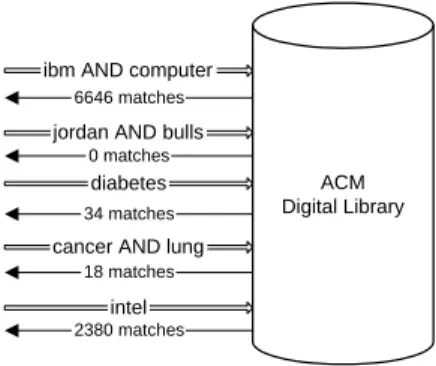
C3=“Health” consisting of the five rules listed in Section 3.1. Suppose that we want to classify the ACM Digital Library database. We send the query ibm AND computer, which re-sults in 6646 matching documents (Figure 2). The other four queries return the matches described in the figure. Us-ing these numbers we estimate that the ACM Digital Li-brary has 0 documents about “Sports,” 6646+2380=9026 documents about “Computers,” and 18+34=52 documents about“Health”. Thus, itsECoverage(ACM) vector for this set of categories is (0,9026,52) and theESpecificity(ACM) vector is 0 0+9026+52, 9026 0+9026+52, 52 0+9026+52 . 2
ACM Digital Library 34 matches 6646 matches 0 matches 18 matches 2380 matches diabetes intel cancer AND lung jordan AND bulls ibm AND computer
Figure 2: Sending probes to the ACM Digital Li-brary database with queries derived from a docu-ment classifier.
3.3
Adjusting Probing Results
Our goal is to get the exact number of documents in each category for a given database. Unfortunately, if we use clas-sifiers to automate this process, then the final result may not be perfect. Classifiers can misclassify documents into incorrect categories, and may not classify some documents at all if those documents do not match any rules. Thus, we need to adjust our initial probing results to account for such potential errors.
It is common practice in the machine learning community to report the document classification results as aconfusion matrix [21]. We adapt this notion of a confusion matrix to match our probing scenario:
Definition 6.: The normalized confusion matrix M = (mij) of a set of query probes for categoriesC1, . . . , Cnis an
n×nmatrix, wheremijis the probability of a document in categoryCjbeing counted as a match by a query probe for categoryCi. Usually,Pn
i=1mij6= 1 because there is a non-zero probability that a document from Cj will not match any query probe.2
The algorithm to create the normalized confusion matrix
M is:
1. Generate the query probes from the classifier rules and probe a database of unseen, preclassified documents (i.e., the test set).
2. Create an auxiliary confusion matrix X = (xij) and set xij equal to the number of documents from Cj that were retrieved from probes ofCi.
3. Normalize the columns ofXby dividing columnjwith the number of documents in the test set in category
Cj. The result is the normalized confusion matrixM. Example 4.: Suppose that we have a document clas-sifier for categories C1=“Sports,” C2=“Computers,” and
C3=“Health.” Consider 5100 unseen, pre-classified ments with 1000 documents about “Sports,” 2500 docu-ments about “Computers,” and 1600 docudocu-ments about “He-alth.” After probing this set with the query probes gener-ated from the classifier, we construct the following confusion matrix: M = 0 B @ 600 1000 100 2500 200 1600 100 1000 2000 2500 150 1600 50 1000 200 2500 1000 1600 1 C A= 0 @ 00..60 010 0..0480 00.09375.125 0.05 0.08 0.625 1 A
Elementm23= 1600150 indicates that 150C3 documents mis-takenly matched probes of C2 and that there are a total of 1600 documents in categoryC3. The diagonal of the matrix gives the probability that documents that matched query probes were assigned to the correct category. For example,
m11 = 1000600 indicates that the probability that aC1 docu-ment is correctly counted as a match for a query probe for
C1 is 0.6. 2
Interestingly, multiplying the confusion matrix with the Coverage vector representing the correct number of docu-ments for each category in the test set yields, by definition, theECoveragevector with the number of documents in each category in the test set as matched by the query probes.
Example 4.: (cont.) TheCoverage vector with the ac-tual number of documents in the test setT for each category is Coverage(T)= (1000,2500,1600). By multiplyingM by this vector we get the distribution of T documents in the categories as estimated by the query probing results.
0 @ 00..60 010 0..0480 00.09375.125 0.05 0.08 0.625 1 A | {z } M × 0 @ 10002500 1600 1 A | {z } Coverage(T) = 0 @ 2250900 1250 1 A | {z } ECoverage(T) 2
Proposition 1.: The normalized confusion matrixM is invertible when the document classifier used to generate M classifies each document correctly with probability>0.5. 2
Proof: From the assumption on the document classifier, it
follows thatmii>Pnj=0,i6=jmij. Hence,M is adiagonally dominant matrix with respect to columns. Then the Gersh-gorin disk theorem [14] indicates thatM is invertible. 2
We note that the condition that a classifier have better than 0.5 probability of correctly classifying each document is in most cases true, but a full discussion of this point is beyond the scope of this paper.
Proposition 1, together with the observation in Exam-ple 4, suggests a way to adjust probing results to compen-sate for classification errors. More specifically, for an unseen databaseDthat follows the data distribution in our training collections it follows that:
M×Coverage(D) ∼= ECoverage(D) Then, multiplying byM−1we have:
Coverage(D) ∼= M−1×ECoverage(D)
Hence, during the classification of a database D, we will multiply M−1 by the probing results summarized in vec-torECoverage(D) to obtain a better approximation of the actual Coverage(D) vector. We will refer to this adjust-ment technique as Confusion Matrix Adjustment or CMA for short.
3.4
Using Probing Results for Classification
So far we have seen how to accurately approximate the document category distribution in a database. We now de-scribe a probing strategy to classify a database using these results.
We classify databases in a top-to-bottom way. Each data-base is first classified by the root-level classifier and is then recursively “pushed down” to the lower level classifiers. A
databaseD is pushed down to the category Cj when both ESpecificity(D,Cj) and ECoverage(D,Cj) are no less than both threshold τes (for specificity) and τec (for coverage), respectively. These thresholds will typically be equal to the
τs and τc thresholds used for the Ideal classification. The final set of categories in which we classifyD is the approxi-mate classification ofDinC.
Definition 7.: Consider a classification schemeC with categoriesC1, . . . , Cnand a searchable web databaseD. If ESpecificity(D) and ECoverage(D)are the approximations of the idealSpecificity(D)andCoverage(D)vectors, respec-tively, the approximate classification of D in C, Approxi-mate(D), consists of each categoryCi such that:
• ESpecificity(D, Ci)≥τes.
• ESpecificity(D, Cj)≥τesfor all ancestorsCjofCi.
• ECoverage(D, Ci)≥τec.
• ECoverage(D, Cj)≥τec for all ancestorsCj ofCi.
• ECoverage(D, Ck) < τec orESpecificity(D, Ck) < τes for all childrenCk ofCi.
with 0≤τes≤1 andτec≥1 given thresholds. 2
The algorithm that computes this set is in Figure 3. To classify a databaseDin a hierarchical classification scheme, we callClassify(“root”, D).
Classify(CategoryC, DatabaseD){
Result =∅
if (C is a leaf node) then return C
Probe databaseD with the query probes derived from the classifier for the subcategories ofC
CalculateECoverage from the number of matches for the probes.
ECoverage(D)=M−1×ECoverage(D)// CMA Calculate theESpecificity vector forC
for all subcategoriesCiofC
if (ESpecificity(D, Ci)≥τesAND ECoverage(D, Ci)≥τec)
thenResult = Result∪Classify(Ci,D) if (Result ==∅)
then return C//Dwas not “pushed” down else return Result
}
Figure 3: Algorithm for classifying a databaseDinto
the category subtree rooted at categoryC.
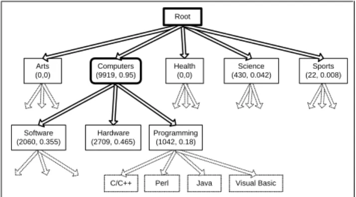
Example 5.: Figure 4 shows how we categorized the ACM Digital Library database. Each node is annotated with theECoverage andESpecificity estimates determined from query probes. The subset of the hierarchy that we explored with these probes depends on theτesand τec thresholds of choice, which for this case were τes = 0.5 and τec = 100. For example, the subtree rooted at node “Science” was not explored, because theESpecificity of this node, 0.042, is less thanτes. Intuitively, although we estimated that around 430 documents in the collection are generally about “Science,” this was not the focus of the database and hence the low ES-pecificity value. In contrast, the “Computers” subtree was further explored because of its highECoverage (9919) and ESpecificity (0.95), but not beyond its children, since their ESpecificity values are less thanτes. Hence the database is classified inApproximate={“Computers”}. 2
C/C++ Perl Java Visual Basic Arts (0,0) Sports (22, 0.008) Science (430, 0.042) Health (0,0) Programming (1042, 0.18) Hardware (2709, 0.465) Software (2060, 0.355) Computers (9919, 0.95) Root
Figure 4: Classifying the ACM Digital Library
database.
4.
EXPERIMENTAL SETTING
We now describe the data (Section 4.1), techniques we compare (Section 4.2), and metrics (Section 4.3) of our ex-perimental evaluation.
4.1
Data Collections
To evaluate our classification techniques, we first define a comprehensive classification scheme (Section 2.1) and then build text classifiers using a set of preclassified documents. We also specify the databases over which we tuned and tested our probing techniques.
Rather than defining our own classification scheme arbi-trarily from scratch we instead rely on that of existing di-rectories. More specifically, for our experiments we picked the five largest top-level categories from Yahoo!, which were also present in InvisibleWeb. These categories are “Arts,” “Computers,” “Health,” “Science,” and“Sports.” We then expanded these categories up to two more levels by selecting the four largest Yahoo! subcategories also listed in Invisi-bleWeb. (InvisibleWeb largely agrees with Yahoo! on the top-level categories in their classification scheme.) The re-sulting three-level classification scheme consists of 72 cate-gories, 54 of which are leaf nodes in the hierarchy. A small fraction of the classification scheme was shown in Figure 4. To train a document classifier over our hierarchical clas-sification scheme we used postings from newsgroups that we judged relevant to our various leaf-level categories. For example, the newsgroupscomp.lang.candcomp.lang.c++ were considered relevant to category “C/C++.” We col-lected 500,000 articles from April through May 2000. 54,000 of these articles, 1000 per leaf category, were used to train RIPPER to produce a rule-based document classifier, and 27,000 articles were set aside as a test collection for the clas-sifier (500 articles per leaf category). We used the remaining 419,000 articles to build controlled databases as we report below.
To evaluate database classification strategies we use two kinds of databases: “Controlled” databases that we assem-bled locally and that allowed us to perform a variety of so-phisticated studies, and real“Web”databases:
Controlled Database Set:We assembled 500 databases
using 419,000 newsgroup articles not used in the classifier training. As before, we assume that each article is labeled with one category from our classification scheme, accord-ing to the newsgroup where it originated. Thus, an article from newsgroupscomp.lang.corcomp.lang.c++will be re-garded as relevant to category “C/C++,” since these news-groups were assigned to category “C/C++.” The size of the
500Controlled databases that we created ranged from 25 to 25,000 documents. Out of the 500 databases, 350 are “ho-mogeneous,” with documents from a single category, while the remaining 150 are “heterogeneous,” with a variety of cat-egory mixes. We define a database as “homogeneous” when it has articles from only one node, regardless of whether this node is a leaf node or not. If it is not a leaf node, then it has equal number of articles from each leaf node in its subtree. The “heterogeneous” databases, on the other hand, have documents from different categories that reside in the same level in the hierarchy (not necessarily siblings), with differ-ent mixture percdiffer-entages. We believe that these databases model real-world searchable web databases, with a variety of sizes and foci. These databases were indexed and queried by a SMART-based program [25] supporting both boolean and vector-space retrieval models.
Web Database Set: We also evaluate our techniques
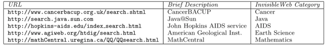
on real web-accessible databases over which we do not have any control. We picked the first five databases listed in the InvisibleWeb directory under each node in our classi-fication scheme (recall that our classiclassi-fication scheme is a portion of InvisibleWeb). This resulted in 130 real web databases. (Some of the lower level nodes in the classifi-cation scheme have fewer than five databases assigned to them.) 12 databases out of the 130 have articles that were “newsgroup style” discussions similar to the databases in theControlled set, while the other 118 databases have arti-cles of various styles, ranging from research papers to film reviews. For each database in theWeb set, we constructed a simple wrapper to send a query and get back the num-ber of matches for each query, which is the only information that our database classification procedure requires. Table 1 shows a sample of five databases from theWeb set.
4.2
Techniques for Comparison
We tested variations of our probing technique, which we refer to as“Probe and Count,”against two alternative stra-tegies. The first one is an adaptation of the technique de-scribed in [2], which we refer to as “Document Sampling.” The second one is a method described in [29] that was specif-ically designed for database classification. We will refer to this method as “Title-based Querying.” The methods are described in detail below.
Probe and Count (PnC): This is our technique,
de-scribed in Section 3, which uses a document classifier for each internal node of our hierarchical classification scheme. Several parameters and options are involved in the training of the document classifiers. For feature selection, we start by eliminating from consideration any word in a list of 400 very frequent words (e.g., “a”, “the”) from the SMART [25] information retrieval system. We then further eliminate all infrequent words that appeared in fewer than three docu-ments. We treated the root node of the classification scheme as a special case, since it covers a much broader spectrum of documents. For this node, we only eliminated words that appeared in fewer than five documents. Also, we consid-ered applying the information theoretic feature selection al-gorithm from [16, 15]. We studied the performance of our system without this feature selection step (FS=off) or with this step, in which we kept only the top 10% most discrim-inating words (FS=on). The main parameters that can be varied in our database classification technique are thresholds
τec (for coverage) andτes(for specificity). Different values for these thresholds result in different approximations
Ap-proximate(D)of the ideal classificationIdeal(D).
Document Sampling (DS):Callan et al. [2] use query
probing to automatically construct a “language model” of a text database (i.e., to extract the vocabulary and associated word-frequency statistics). Queries are sent to the database to retrieve a representative random document sample. The documents retrieved are analyzed to extract the words that appear in them. Although this technique was not designed for database classification, we decided to adapt it to our task as follows:
1. Pick a random word from a dictionary and send a one-word query to the database in question.
2. Retrieve the top-N documents returned by the data-base for the query.
3. Extract the words from each document and update the list and frequency of the words accordingly.
4. If a termination condition is met, go to Step 5; else go to Step 1.
5. Use a modification of the algorithm in Figure 3 that “probes” the sample document collection rather than the database itself.
For Step 1, we use a random word from the approximately 100,000 words in our newsgroup collection. For Step 2, we useN= 4, which is the value that Callan et al. recommend in [2]. Finally, we use the termination condition in Step 4 also as described in [2]: the algorithm terminates when the vocabulary and frequency statistics associated with the sample document collection converge to a reasonably stable state (see [2] for details). At this point, the adapted tech-nique can proceed almost identically as in Section 3.4 by probing the locally stored document sample rather than the original database. A crucial difference between the Docu-ment Sampling technique and our Probe and Count tech-nique is that we only use the number of matches reported by each database, while theDocument Sampling technique requires retrieving and analyzing the actual documents from the database for the key Step 4 termination condition test.
Title-based Querying (TQ):Wang et al. [29] present
three different techniques for the classification of searchable web databases. For our experimental evaluation we picked the method they deemed best. Their technique creates one long query for each category using the title of the category itself (e.g., “Baseball”) augmented by the titles of all of its subcategories. For example, the query for category “Base-ball” is“baseball mlb teams minor leagues stadiums statis-tics college university...” The query for each category is sent to the database in question, the top ranked results are retrieved, and the average similarity [25] of these documents and the query defines the similarity of thedatabasewith the category. The database is then classified into the categories that are most similar with it. The details of the algorithm are described below.
1. For each categoryCi:
(a) Create an associated “concept query,” which is simply the title of the category augmented with the titles of its subcategories.
(b) Send the“concept query”to the database in ques-tion.
(c) Retrieve the top-N documents returned by the database for this query.
(d) Calculate the similarity of these N documents with the query. The average similarity will be the similarity of the database with categoryCi.
URL Brief Description InvisibleWeb Category
http://www.cancerbacup.org.uk/search.shtml CancerBACUP Cancer
http://search.java.sun.com Java@Sun Java
http://hopkins-aids.edu/index search.html John Hopkins AIDS service AIDS
http://www.agiweb.org/htdig/search.html American Geological Inst. Earth Science
http://mathCentral.uregina.ca/QQ/QQsearch.html MathCentral Mathematics
Table 1: Some of the real web databases in the Web set.
2. Rank the categories in order of decreasing similarity with the database.
3. Assign the database to the top-K categories of the hierarchy.
To create the concept queries of Step 1, we augmented our hierarchy with an extra level of “titles,” as described in [29]. For Step 1(c) we used the valueN = 10, as recommended by the authors. We used the cosine similarity function with tf.idf weighting [24]. Unfortunately, the value ofKfor Step 3 is left as an open parameter in [29]. We decided to fa-vor this technique in our experiments by “revealing” to it the correct number of categories into which each database should be classified. Of course this information would not be available in a real setting, and was not provided to our Probe and Count or theDocument Sampling techniques.
4.3
Evaluation Metrics
To quantify the accuracy of category frequency estimates for databaseDwe measure the absolute error (i.e., Manhat-tan disManhat-tance) between the approximation vectors ECover-age(D)and ESpecificity(D), and the correct vectors Cover-age(D) and Specificity(D). These metrics are especially re-vealing during tuning (Section 5.1). The error metric alone, however, cannot give an accurate picture of the system’s performance, since the main objective of our system is to classify databases correctly and not to estimate the Speci-ficityandCoveragevectors, which are only auxiliary for this task.
We evaluate classification algorithms by comparing the approximate classification Approximate(D) that they pro-duce against the ideal classificationIdeal(D). We could just report the fraction of the categories inApproximate(D)that are correct (i.e., that also appear inIdeal(D)). However, this would not capture the nuances of hierarchical classification. For example, we may have classified a database in category “Sports,” while it is a database about “Basketball.” The metric above would consider this classification as absolutely wrong, which is not appropriate since, after all, “Basket-ball” is a subcategory of “Sports.” With this in mind, we adapt theprecision andrecall metrics from information re-trieval [3]. We first introduce an auxiliary definition. Given a set of categoriesN, we “expand” it by including all the subcategories of the categories inN. ThusExpanded(N)=
{c ∈ C|c ∈ N or c is in a subtree of somen ∈ N}. Now, we can defineprecision andrecall as follows.
Definition 8.: Consider a databaseDclassified into the set of categoriesIdeal(D), and an approximation ofIdeal(D) given inApproximate(D).LetCorrect = Expanded(Ideal(D)) andClassified = Expanded(Approximate(D)). Then the pre-cision andrecall of the approximate classification ofDare:
precision = |Correct∩Classified|
|Classified|
recall = |Correct∩Classified|
|Correct|
2
To condense precision and recall into one number, we use theF1-measure metric [28],
F1 = 2×precision×recall
precision+recall
which is only high when both precision and recall are high, and is low for design options that trivially obtain high pre-cision by sacrificing recall or vice versa.
Example 6.: Consider the classification scheme in Fig-ure 4. Suppose that the ideal classification for a database
D isIdeal(D)={“Programming”}. Then, theCorrect set of categories include “Programming” and all its subcategories, namely “C/C++,” “Perl,” “Java,” and “Visual Basic.” If we approximateIdeal(D)asApproximate(D)={“Java”} us-ing the algorithm in Figure 3, then we do not manage to cap-ture all categories inCorrect. In fact we miss four out of five such categories and hencerecall=0.2 for this database and approximation. However, the only category in our approx-imation, “Java,” is a correct one, and hence precision=1. TheF1-measure summarizesrecallandprecisionin one num-ber,F1= 2×1+0.21×0.2 = 0.33. 2
An important property of classification strategies over the web is scalability. We measure the efficiency of the var-ious techniques that we compare by modelling their cost. More specifically, the maincost we quantify is the number of “interactions” required with the database to be classified, where each interaction is either a query submission (needed for all three techniques) or the retrieval of a database docu-ment (needed only forDocument Sampling andTitle-based Querying). Of course, we could include other costs in the comparison (namely, the cost of parsing the results and pro-cessing them), but we believe that they would not affect our conclusions, since these costs are CPU-based and small compared to the cost of interacting with the databases over the Internet.
5.
EXPERIMENTAL RESULTS
We now report experimental results that we used to tune our system (Section 5.1) and to compare the different clas-sification alternatives both for the Controlled database set (Section 5.2) and for theWeb database set (Section 5.3).
5.1
Tuning the Probe and Count Technique
Our Probe and Count technique has some open param-eters that we tuned experimentally by using a set of 100 Controlled databases (Section 4.1). These databases will not participate in any of the subsequent experiments.
Effect of Confusion Matrix Adjustment (CMA):
The first parameter we examined was whether the confu-sion matrix adjustment of the probing results was helpful or not. The absolute error associated with theECoverage and ESpecificity approximations was consistently smaller when
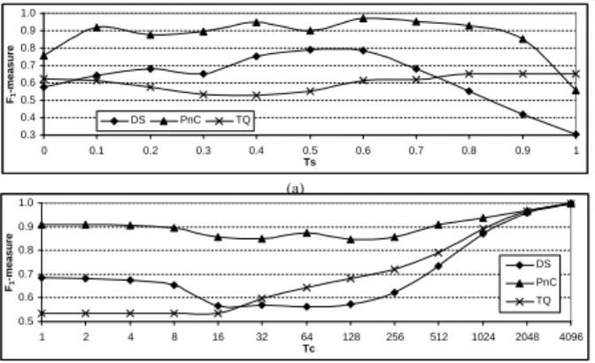
0.3 0.4 0.5 0.6 0.7 0.8 0.9 1.0 0 0.1 0.2 0.3 0.4 0.5 0.6 0.7 0.8 0.9 1 Ts F1 -measure DS PnC TQ (a) 0.5 0.6 0.7 0.8 0.9 1.0 1 2 4 8 16 32 64 128 256 512 1024 2048 4096 Tc F1 -measure DS PnC TQ (b)
Figure 5: The average F1-measure of the three
techniques (a) for varying specificity threshold τs
(τc = 8), and (b) for varying coverage threshold τc
(τs= 0.3).
we used CMA, confirming our motivation behind the intro-duction of CMA. (Due to lack of space we do not report this plot.) Consequently, we fix this parameter and use confusion matrix adjustment for all the remaining experiments.
Effect of Feature Selection: As we described in
Sec-tion 4.2, we can apply an informaSec-tion theoretic feature se-lection step before training a document classifier. We ran our Probe and Count techniques with (FS=on) and with-out (FS=off) this feature selection step. The estimates of both theCoverageandSpecificityvectors that we computed withFS=onwere consistently more accurate than those for FS=off. More specifically, the ECoverage estimates with FS=on were between 15% and 20% better, while the ES-pecificity estimates with FS=on were around 10% better. (Again, due to space restrictions we do not include more detailed results.) Intuitively, our information theoretic fea-ture selection step results in robust classifiers that use fewer “noisy” terms for classification. Consequently, we fix this parameter and useFS=onfor all the remaining experiments. We now turn to reporting the results of the experimental comparison ofProbe and Count, Document Sampling, and Title-based Querying over the 400 unseen databases in the Controlled set and the 130 databases in theWebset.
5.2
Results over the Controlled Databases
Accuracy for Differentτs andτcThresholds: As
ex-plained in Section 2.2, Definition 3, the ideal classification of a database depends on two parameters: τs (for specificity) andτc(for coverage). The values of these parameters are an “editorial decision” and depend on whether we decide that our classification scheme is specificity- or coverage-oriented, as discussed previously. To classify a database, both the Probe and Count and Document Sampling techniques need analogous thresholdsτes andτec. We ran experiments over the Controlled databases for different combinations of the
τs and τc thresholds, which result in different ideal classi-fications for the databases. Intuitively, for low specificity thresholdτs theIdeal classification will have the databases assigned mostly to leaf nodes, while a high specificity thresh-old might lead to databases being classified at more general nodes. Similarly, low coverage thresholdsτc produce Ideal classifications where the databases are mostly assigned to the leaves, while higher values ofτctend to produce classi-fications with the databases assigned to higher level nodes. For Probe and Count and Document Sampling we set
τes=τsandτec=τc.Title-based Queryingdoes not use any such threshold, but instead needs to decide how many cate-goriesKto assign a given database (Section 4.2). Although of course the value ofK would be unknown to a classifica-tion technique (unlike the values for thresholdsτs and τc), we revealK to this technique, as discussed in Section 4.2.
Figure 5(a) shows the average value of theF1-measure for
varyingτs and forτc= 8, over the 400 unseen databases in theControlled set. The results were similar for other values ofτcas well. Probe and Count performs the best for a wide range ofτsvalues. The only case in which it is outperformed byTitle-based Queryingis whenτs= 1. For this setting even very small estimation errors forProbe and Countand Docu-ment Samplingresult in errors in the database classification (e.g., even if Probe and Count estimates 0.9997 specificity for one category it will not classify the database into that category, due to its “low specificity”). Unlike Document Sampling,Probe and Count (except forτs= 1 andτs = 0) andTitle-based Queryinghave almost constant performance for different values ofτs.Document Samplingis consistently worse thanProbe and Count, showing that sampling using random queries is inferior than using a focused, carefully chosen set of queries learned from training examples.
Figure 5(b) shows the average value of the F1-measure
for varyingτc and for τs = 0.3. The results were similar for other values ofτs as well. Again,Probe and Count out-performs the other alternatives and, except for low cover-age thresholds (τc≤16),Title-based Querying outperforms Document Sampling. It is interesting to see that the per-formance ofTitle-based Querying improves as the coverage thresholdτcincreases, which might indicate that this scheme is better suited for coverage-based classification schemes.
Effect of Depth of Hierarchy in Accuracy: An
inter-esting question is whether classification performance is af-fected by the depth of the classification hierarchy. We tested the different methods against “adjusted” versions of our hi-erarchy of Section 4.1. Specifically, we first used our original classification scheme with three levels (level=3). Then we eliminated all the categories of the third level to create a shallower classification scheme (level=2). We repeated this process again, until our classification schemes consisted of one single node (level=0). Of course, the performance of all the methods at this point was perfect. In Figure 6 we com-pare the performance of the three methods forτs= 0.3 and τc= 8 (the trends were the same for other threshold com-binations as well). Probe and Count performs better than the other techniques for different depths, with only a smooth degradation in performance for increasing depth, which sug-gests that our approach can scale to a large number of cate-gories. On the other hand,Document Sampling outperforms Title-based Queryingbut for both techniques the difference in performance withProbe and Count increases for hierar-chies of larger depth.
Efficiency of the Classification Methods: As we
dis-cussed in Section 4.3, we compare the number of queries sent to a database during classification and the number of documents retrieved, since the other costs involved are com-parable for the three methods. The Title-based Querying technique has a constant cost for each classification: it sends one query for each category in the classification scheme and retrieves 10 documents from the database. Thus, this tech-nique sends 72 queries and retrieves 720 documents for our 72-node classification scheme. OurProbe and Count tech-nique sends a variable number of queries to the database
0.50 0.55 0.60 0.65 0.70 0.75 0.80 0.85 0.90 0.95 1.00 0 1 2 3 Level F1 -measure DS PnC TQ
Figure 6: The averageF1-measure for hierarchies of
different depths (τs= 0.3,τc= 8). 500 750 1000 1250 1500 1750 2000 0 0.1 0.2 0.3 0.4 0.5 0.6 0.7 0.8 0.9 1 Tes
Interactions with Database
PnC DS TQ (a) 250 500 750 1000 1250 1500 1750 2000 1 2 4 8 16 32 64 128 256 512 1024 2048 4096 8192 Tec
Interactions with Database
PnC DS TQ
(b)
Figure 7: The average number of “interactions” with the databases (a) as a function of threshold
τes (τec = 8), and (b) as a function of threshold τec
(τes= 0.3).
being classified. The exact number depends on how many times the database will be “pushed” down a subcategory (Figure 3). Our technique does not retrieve any documents from the database. Finally, theDocument Samplingmethod sends queries to the database and retrieves four documents for each query until the termination condition is met. We list in Figure 7(a) the average number of “interactions” for varying values of specificity threshold τes and τec = 8. Figure 7(b) shows the average number of “interactions” for varying coverage threshold τec and τes = 0.3. Docu-ment Sampling is consistently the most expensive method, while Title-based Querying performs fewer “interactions” thanProbe and Count for low values for specificity thresh-oldτesandτec, whenProbe and Count tends to push down databases more easily, which in turn translates into more query probes.
In summary,Probe and Countis by far the most accurate method. Furthermore, its cost is lowest for most combina-tions of theτes andτec thresholds and only slightly higher than the cost ofTitle-based Querying, a significantly less ac-curate technique, for the remaining combinations. Finally, theProbe and Count query probes are short, consisting on average of only 1.5 words, with a maximum of four words. In contrast, the average Title-based Querying query probe consisted of 18 words, with a maximum of 348 words.
5.3
Results over the Web Databases
The experiments over the Web databases involved only
1 4 16 64 256 1024 4096 16384 65536 262144 0 0.2 0.4 0.6 0.8 1 0 0.1 0.2 0.3 0.4 0.5 0.6 0.7 0.8 F1 -measure Tec Tes
Figure 8: Average F1-measure values for different
combinations ofτes andτec.
theProbe and Count technique. The main reason for this was the prohibitive cost of running such experiments for theDocument Sampling and theTitle-based Querying tech-niques, which would have required constructing “wrappers” for each of the 130 databases in the Web set. Such wrap-pers would have to extract all necessary document pointers from result pages from each query probe returned by the database, so defining them involves non-trivial human effort. In contrast, the “wrappers” needed by theProbe and Count technique are significantly simpler, which is a major advan-tage of our approach. As we will discuss in Section 7, the Probe and Countwrappers only need to extract the number of matches from each results page, a task that could be au-tomated since the patterns used by search engines to report the number of matches for queries are quite uniform.
For the experiments over theControlled set, the classifi-cation thresholds τs and τc of choice were known. In con-trast, for the databases in theWebset we are assuming that theirIdeal classification is whatever categories were chosen (manually) by the InvisibleWeb directory (Section 4.1). This classification of course does not use theτs andτcthresholds in Definition 3, so we cannot use these parameters as in theControlled case. However, we assume that InvisibleWeb (and any consistent categorization effort) implicitly uses the notion of specificity and coverage thresholds for their clas-sification decisions. Hence we try and learn such thresholds from a fraction of the databases in the Web set, use these values as the τes and τec thresholds forProbe and Count, and validate the performance of our technique over the re-maining databases in theWeb set.
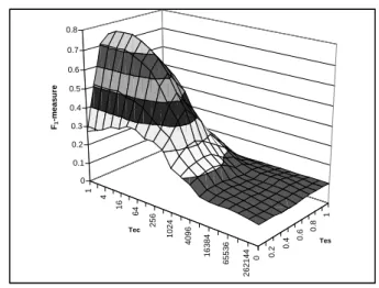
Accuracy for DifferentτsandτcThresholds: For the
Web set, the Ideal classification for each database is taken from InvisibleWeb. To find the τs andτc that are “implic-itly used” by human experts at InvisibleWeb we have split the Web set in three disjoint sets W1, W2, and W3. We
first use the union of W1 andW2 to learn these values of
τs andτc by exhaustively exploring a number of combina-tions and picking theτesandτecvalue pair that yielded the bestF1-measure (Figure 8). As we can see, the best values
corresponded to τes = 0.3 and τec = 16, with F1 = 0.77.
To validate the robustness of the conclusion, we tested the performance ofProbe and Countover the third subset of the Webset,W3: for these values ofτesandτectheF1-measure
Training Subset Learnedτs,τc F1-measure over Train-ing Subset Test
Subset Fover1-measureTest Subset
W1∪W2 0.3, 16 0.77 W3 0.79
W1∪W3 0.3, 8 0.78 W2 0.75
W2∪W3 0.3, 8 0.77 W1 0.77
Table 2: Results of three-fold cross-validation over
theWeb databases.
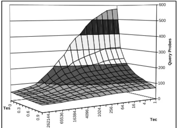
1 4 16 64 256 1024 4096 16384 65536 262144 0 0.3 0.6 0.9 0 100 200 300 400 500 600 Query Probes Tec Tes
Figure 9: Average number of query probes for the
Web databases as a function of τesand τec.
over the unseenW3 set was 0.79, very close to the one over training setsW1,W2. Hence, the training to find theτsand
τc values was successful, since the pair of thresholds that we found performs equally well for the InvisibleWeb catego-rization of unseen web databases. We performed three-fold cross-validation [21] for this threshold learning by training onW2 and W3 and testing onW1, and finally learning on
W1andW3 and testing onW2. Table 2 summarizes the re-sults. The results were consistent, confirming the fact that the values ofτes = 0.3 andτec ≈8 are not overfitting the databases in ourWebset.
Effect of Depth of Hierarchy in Accuracy: We also
tested our method for hierarchical classification schemes of various depths usingτes= 0.3 andτec= 8. TheF1-measure was 1, 0.89, 0.8, and 0.75 for hierarchies of depth zero, one, two, and three respectively. We can see that F1-measure drops smoothly as the hierarchy depth increases, which leads us to believe that our method can scale to even larger clas-sification schemes without significant penalties in accuracy.
Efficiency of the Classification Method: The cost of
the classification for the different combinations of the thresh-olds is depicted in Figure 9. As the threshthresh-olds increase, the number of queries sent decreases, as expected, since it is more difficult to “push” a database down a subcategory and trigger another probing phase. The cost is generally low: only a few hundred queries suffice on average to classify a database with high accuracy. Specifically, for the best set-ting of thresholds (τs = 0.3 and τc = 8), the Probe and Count method sends on average only 185 query probes to each database in theWebset. As we mentioned, the average query probe consists of only 1.5 words.
6.
RELATED WORK
While work in text database classification is relatively new, there has been substantial on-going research in text documentclassification. Such research includes the applica-tion of a number of learning algorithms to categorizing text documents. In addition to the rule-based classifiers based
on RIPPER used in our work, other methods for learning classification rules based on text documents have been ex-plored [1]. Furthermore, many other formalisms for doc-ument classifiers have been the subject of previous work, including the Rocchio algorithm based on the vector space model for document retrieval [23], linear classification al-gorithms [17], Bayesian networks [18], and, most recently, support vector machines [13], to name just a few. More-over, extensive comparative studies among text classifiers have also been performed [26, 7, 31], reflecting the relative strengths and weaknesses of these various methods.
Orthogonally, a large body of work has been devoted to the interaction with searchable databases, mainly in the form of metasearchers [9, 19, 30]. A metasearcher receives a query from a user, selects the best databases to which to send the query, translates the query in a proper form for each search interface, and merges the results from the different sources.
Query probing has been used in this context mainly for the problem of database selection. Specifically, Callan et al. [2] probe text databases with random queries to deter-mine an approximation of their vocabulary and associated statistics (“language model”). (We adapted this technique for the task of database classification to define the Docu-ment Sampling technique of Section 4.2.) Craswell et al. [5] compared the performance of different database selec-tion algorithms in the presence of such “language models.” Hawking and Thistlewaite [11] used query probing to per-form database selection by ranking databases by similarity to a given query. Their algorithm assumed that the query interface can handle normal queries and query probes dif-ferently and that the cost to handle query probes is smaller than that for normal queries. Recently, Etzioni and Sug-iura [27] used query probing for query expansion to route web queries to the appropriate search engines.
Query probing has also been used for other tasks. Meng et al. [20] used guided query probing to determine sources of heterogeneity in the algorithms used to index and search locally at each text database. Query probing has been used by Etzioni et al. [22] to automatically understand query forms and extract information from web databases to build a comparative shopping agent. In [10] query probing was employed to determine the use of different languages on the web.
For the task of database classification, Gauch et al. [8] manually construct query probes to facilitate the classifica-tion of text databases. In [12] we presented preliminary work on database classification through query probes, on which this paper builds. Weng et al. [29] presented theTitle-based Querying technique that we described in Section 4.2. Our experimental evaluation showed that our technique signif-icantly outperforms theirs, both in terms of efficiency and effectiveness. Our technique also outperforms our adapta-tion of the random document sampling technique in [2].
7.
CONCLUSIONS AND FUTURE WORK
We have presented a novel and efficient method for the hi-erarchical classification of text databases on the web. After providing a more formal description of this task, we pre-sented a scalable algorithm for the automatic classification of such databases into a topic hierarchy. This algorithm employs a number of steps, including the learning of a rule-based classifier that is used as the foundation for generat-ing query probes, a method for adjustgenerat-ing the result counts
returned by the queried database, and finally a decision cri-terion for making classification assignments based on this adjusted count information. Our technique does not require retrieving any documents from the database. Experimental results show that the method proposed here is both more accurate and efficient than existing methods for database classification.
While in our work we focus on rule-based approaches, we note that other learning algorithms are directly applicable in our approach. A full discussion of such transformations is beyond the scope of this paper. We simply point out that the database classification scheme we present is not bound to a single learning method, and may be improved by simul-taneous advances from the realm of document classification. A further step that would completely automate the classi-fication process is to eliminate the need for a human to con-struct the simple wrapper for each database to classify. This step can be eliminated by automatically learning how to parse the pages with query results. Perkowitz et al. [22] have studied how to automatically characterize and understand web forms, and we plan to apply some of these results to automate the interaction with search interfaces. Our tech-nique is particularly well suited for this automation, since it needs only very simple information from result pages (i.e., the number of matches for a query). Furthermore, the pat-terns used to report the number of matches for queries by the search engines and tools that are popular on the web are quite similar. For example, one representative pattern is the appearance of the word “of” before reporting the actual number of matches for a query (e.g., “30 outof 1024 matches displayed”). 76 out of the 130 web databases in theWebset use this pattern to report the number of matches, and of course there are other common patterns as well. Based on this anecdotal information, it seems realistic to envision a completely automatic classification system.
Acknowledgments
Panagiotis G. Ipeirotis is partially supported by Empeiri-keio Foundation and he thanks the Trustees of EmpeiriEmpeiri-keio Foundation for their support. We also thank Pedro Falcao Goncalves for his contributions during the initial stages of this project. This material is based upon work supported by the National Science Foundation under Grants No. IIS-97-33880 and IIS-98-17434. Any opinions, findings, and con-clusions or recommendations expressed in this material are those of the authors and do not necessarily reflect the views of the National Science Foundation.
8.
REFERENCES
[1] C. Apte, F. Damerau, and S. M. Weiss. Automated learning of decision rules for text categorization.Transactions of Office
Information Systems, 12(3), 1994.
[2] J. P. Callan, M. Connell, and A. Du. Automatic discovery of
language models for text databases. InSIGMOD 1999,
Proceedings ACM SIGMOD International Conference on
Management of Data, pages 479–490, 1999.
[3] C. W. Cleverdon and J. Mills. The testing of index language devices.Aslib Proceedings, 15(4):106–130, 1963.
[4] W. W. Cohen. Learning trees and rules with set-valued features. InProceedings of AAAI’96, IAAI’96, volume 1, pages 709–716. AAAI, 1996.
[5] N. Craswell, P. Bailey, and D. Hawking. Server selection on the
World Wide Web. InProceedings of the Fifth ACM
Conference on Digital Libraries, pages 37–46. ACM, 2000.
[6] The Deep Web: Surfacing Hidden Value. Accessible at
http://www.completeplanet.com/Tutorials/DeepWeb/index.asp. [7] S. T. Dumais, J. Platt, D. Heckerman, and M. Sahami.
Inductive learning algorithms and representations for text
categorization. InProceedings of CIKM-98, 1998. [8] S. Gauch, G. Wang, and M. Gomez. Profusion*: Intelligent
fusion from multiple, distributed search engines.The Journal
of Universal Computer Science, 2(9):637–649, Sept. 1996.
[9] L. Gravano, H. Garc´ıa-Molina, and A. Tomasic.GlOSS:
Text-Source Discovery over t