UNIVERSITÀ DEGLI STUDI DI PADOVA
CORSO DI DOTTORATO IN PSYCHOLOGICAL SCIENCES XXXI CICLO
BAYESIAN MODELING OF TEMPORAL EXPECTATIONS
IN THE HUMAN BRAIN
Supervisore
Prof. Antonino Vallesi
Dottorando Antonino Visalli
ABSTRACT ... 3
GENERAL INTRODUCTION ... 9
1.1 TEMPORAL PREPARATION ... 10
1.2 BAYESIAN BELIEF UPDATING ... 13
1.3 PROJECT OVERVIEW ... 20
TEMPORAL BELIEF UPDATING AND SURPRISE MODULATE COGNITIVE CONTROL NETWORKS ... 23
2.1 INTRODUCTION ... 23
2.2 METHODS ... 26
2.2.1 Participants ... 26
2.2.2 Task and procedure ... 27
2.2.3 Normative Bayesian learner ... 30
2.2.4 Model-based measures of updating and surprise ... 31
2.2.5 Behavioral data analysis ... 34
2.2.6 fMRI data analysis ... 34
2.3 RESULTS ... 38
2.3.1 Behavioral results ... 38
2.3.2 Whole-brain fMRI results ... 39
2.4 DISCUSSION ... 43
ELECTROPHYSIOLOGICAL CORRELATES OF TEMPORAL BELIEF UPDATING AND SURPRISE . 49 3.1 INTRODUCTION ... 49
3.2 METHODS ... 52
3.2.1 Participants ... 52
3.2.2 Task and procedure ... 53
3.2.3 EEG data acquisition ... 54
3.2.4 Normative Bayesian learner and regressors ... 55
3.2.5 EEG data analysis ... 55
3.3 RESULTS ... 57
3.3.1 Behavioral results ... 57
3.3.2 Electrophysiological results ... 58
BEYOND EXPLICIT INFERENCE: EEG CORRELATES OF IMPLICIT UPDATING OF TEMPORAL
EXPECTATIONS ... 69
4.1 INTRODUCTION ... 69
4.2 METHODS ... 71
4.2.1 Participants ... 71
4.2.2 Task and procedure ... 72
4.2.3 Normative Bayesian learner and regressors ... 72
4.2.4 EEG data analysis ... 77
4.3 RESULTS ... 78
4.3.1 Electrophysiological results ... 78
4.3.2 EEG results, between-study comparison ... 78
4.4 DISCUSSION ... 87
GENERAL DISCUSSION ... 93
ACKNOWLEDGEMENTS ... 101
Abstract
The ability to predict when a relevant event might occur is critical to survive in our dynamic and uncertain environment. This cognitive ability, usually referred to as temporal preparation, allows us to prepare temporally optimized responses to
forthcoming stimuli by anticipating their timing: from safely crossing a busy road during rush hours, to timing turn taking in a conversation, to catching something in mid-air, are all examples of how important and ubiquitous temporal preparation is in our everyday life (e.g., Correa, 2010; Coull & Nobre, 2008; Nobre, Correa, & Coull, 2007).
In laboratory settings, temporal preparation has been traditionally investigated, in its implicit form, through the “variable foreperiod paradigm” (see Coull, 2009; Niemi & Näätänen, 1981, for a review). In such a paradigm, the foreperiod is a time interval of variable duration that separates a warning stimulus and a target stimulus requiring a response. What is usually observed with this paradigm is that response times (RTs) reflect the temporal probability of stimulus onset: RTs decrease with increasing probability. This implies that participants learn to use the information implicitly afforded by the passage of time and that related to the temporal probability of the onset of the target stimulus (i.e., hazard rate; Janssen & Shadlen, 2005). In other words, it seems that they are able to use predictive internal models of event timing in order to optimize behaviour.
Despite previous studies have started to investigate which brain areas encode temporal probabilities (i.e., predictive models) to anticipate event onset (e.g., Bueti, Bahrami, Walsh, & Rees, 2010; Cui, Stetson, Montague, & Eagleman, 2009; also see Vallesi et al., 2007), to our knowledge, there is no evidence on how the brain does
form and update such predictive models. Based on such premises, the overarching goal of the present PhD project was to pinpoint the neural mechanisms by which predictive models of event timing are dynamically updated. Moreover, given that in real life updating usually occurs in the presence of surprising events (i.e. low probable events under a predictive model), it is challenging to disentangle between updating and surprise (O’Reilly et al, 2013). Therefore, our second and interrelated research goal was to understand whether, and to which extent, it is possible to dissociate between the neural mechanisms specifically involved in updating and those dealing with surprising events that do not require an update of internal models. To accomplish our research goals, we capitalized on both state-of-the-art methodologies [i.e., functional magnetic resonance imaging (fMRI) and electrophysiology (EEG)] and computational modelling. Specifically, we considered the brain like a Bayesian observer. Indeed, Bayesian frameworks are gaining increasing popularity to explain cognitive brain functions (Friston, 2012). In a nutshell, the construction of computational Bayesian models allows us to quantitatively describe temporal expectations in terms of probability distributions and to capture updating using Bayes’ rule.
In order to accomplish our goals, the present PhD project is composed of three studies. In the first two studies we implemented a version of the foreperiod paradigm in which participants could predict target onsets by estimating their underlying temporal probability distributions. During the task, these distributions changed, hence requiring participants to update their temporal expectations. Furthermore, a simple manipulation of the colors in which the target were presented (cf., O’Reilly et al., 2013) allowed us to independently vary updating and surprise across trials. Then, we constructed a normative Bayesian learner (a computational model adapted from
O’Reilly et al., 2013) in order to obtain an estimate of a participant’s temporal expectations on a trial-by-trial basis. In Study 1, trial-by-trial fMRI data acquired during our foreperiod paradigm were correlated with two information theoretical parameters calculated with reference to our Bayesian model: the Kullbach-Leibler divergence (DKL) and the Shannon’s information (IS). These two measures have been
previously used to formally describe belief updating and surprise associated with events under a predictive model, respectively (e.g., Baldi & Itti, 2010; Kolossa, Kopp, & Fingscheidt, 2015; O'Reilly et al., 2013; Strange et al., 2005). Our results showed that the fronto-parietal network and the cingulo-opercular network were differentially involved in the updating of temporal expectations and in dealing with surprising events, respectively.
Having successfully validated the use of Bayesian models in our first fMRI study and dissociated between updating and surprise, the next step was to investigate the temporal dynamics of these two processes. Do updating and surprise act on similar or distinct processing stage(s)? What is the time course associated with the two? To address these questions, in Study 2 participants performed our adapted foreperiod task (same task as in Study 1) while their EEG activity was recorded. In this study, we relied on the literature on the P3 (a specific ERP component related to information processing) and the Bayesian brain (e.g., Kopp, 2008; Kopp et al., 2016; Mars et al., 2008; Seer, Lange, Boos, Dengler, & Kopp, 2016). Importantly, however, we also took advantage from the combination of a mass-univariate approach with novel deconvolution methods to explore the entire spatio-temporal pattern of EEG data. This enabled us to extend our analyses beyond the P3 component. Results from study 2 confirmed that surprise and updating can be differentiated also at the electrophysiological level and that updating elicited a more complex pattern than
surprise. As regards the P3 in relation to the literature on the Bayesian brain (Kolossa, Fingscheidt, Wessel, & Kopp, 2013; Kolossa et al., 2015; Mars et al., 2008), our findings corroborated the idea that such a component is selectively modulated by surprise and updating.
While in Studies 1 and 2, participants were explicitly encouraged to form and update temporal expectations using the target color, in Study 3 we wanted to make a step further by asking whether the use of a more implicit task structure might influence the construction of the predictive internal model. To that aim, during the foreperiod task designed for the third study, participants were not explicitly informed about the presence of the underlying temporal probability distributions from which target onsets were drawn. In this way, we aimed to investigate behavioural and EEG differences in the way participants learnt to form and updated temporal expectations when changes in the underlying distributions were not explicitly signalled. Critically, we again found that surprise and updating could be differentiated. Moreover, coupled with the results from study 2, we isolated two EEG signatures of the inferential process underlying updating of prior temporal expectations, which responded to both explicit and implicit contextual changes.
Overall, we believe that the results of the present PhD project will further our understanding of the cognitive processes and neural mechanisms that allow us to optimize our temporal preparation abilities.
Chapter 1
General introduction
To get access to my supervisor’s office, I usually take the elevator. On one occasion I was waiting for it together with other people. While I was still entering the elevator, the door “unexpectedly” started to close hitting my shoulder. This embarrassing situation happened again a few times more before I learnt that the waiting interval between door opening and closing was very short and to update my incorrect temporal expectation in such a way to safely enter the elevator in future occasions!
The example above illustrates the importance of the ability to accurately predict the likely moment at which an event might occur in everyday situations, an ability usually labeled “temporal preparation” (Correa, 2010; Nobre, Correa, & Coull, 2007). While previous studies have started to unveil the neural mechanisms by which temporal expectations are updated, a direct modeling of how our brain faces this key task is still poorly estimated. To address this issue, in the present thesis we combined a temporal preparation task with Bayesian modeling during either functional magnetic resonance imaging (fMRI) or electrophysiological (EEG) studies. The reasons why we believe that a Bayesian approach would be particularly suited to investigate temporal preparation are outlined below. Specifically, in order to fully appreciate the rationale behind the work presented here, we will begin by briefly
reviewing the literature on both temporal preparation and Bayesian belief updating. In the last part of the Introduction, we will then present an overview of the project in which we make a link between the literature on temporal preparation and Bayesian models.
1.1 Temporal preparation
In laboratory settings, temporal preparation has been usually studied through the “foreperiod paradigm” (see Coull, 2009; Niemi & Näätänen, 1981, for reviews). The foreperiod is the time interval that separates a warning stimulus from a subsequent target that calls for a fast and accurate response. When the foreperiod duration is kept constant throughout a block of trials (e.g., in one block the target always appears after 500 ms, whereas in another block it does so after 1000 ms), participants’ reaction times (RTs) are usually faster for the short rather than the long block of trials, a phenomenon known as the “fixed foreperiod effect” (e.g., Bausenhart, Rolke, & Ulrich, 2008; Mattes & Ulrich, 1997; Vallesi, McIntosh, Shallice, & Stuss, 2009). However, if short and long foreperiod durations are randomly intermixed across the trials and each one has the same a priori probability of being presented, participants will be faster for targets appearing after long than short foreperiods, i.e., “the variable foreperiod effect” (Niemi & Näätänen, 1981; Woodrow, 1914).
The different findings associated with fixed and variable foreperiod paradigms have been traditionally explained by two mechanisms: time estimation and monitoring the conditional probability of target occurrence, respectively. Since in the fixed paradigm, uncertainty in time estimation will increase as a function of the time interval being estimated (i.e. scalar theory, Gibbon, 1977), it follows that RTs will also increase with longer durations. The scenario instead changes for the variable foreperiod paradigm. Here, as time goes by during the trial and the target has not yet appeared after the shorter foreperiods, participants may infer that it will surely occur after the longest ones, provided that there are no catch trials, which explains the RT advantage for long foreperiod trials. This pattern of data can be
formally described in terms of a mechanism monitoring the hazard function, that is the conditional probability that the target will occur given that it has not yet occurred, and exploiting it to optimize preparation (Nobre et al., 2007).
Converging evidence from fMRI (Vallesi, McIntosh, Shallice, et al., 2009; A. Vallesi, McIntosh, & Stuss, 2009), transcranial magnetic stimulation (Vallesi, Shallice, & Walsh, 2007), and neuropsychological studies (Stuss et al., 2005; Trivino, Correa, Arnedo, & Lupianez, 2010; Vallesi et al., 2007) points to the involvement of prefrontal areas, in particular the right dorsolateral prefrontal cortex, in the variable foreperiod effect. However, these studies most often used few discrete foreperiod durations (e.g., two), which makes it difficult to model how behavioural and neural responses are shaped by the hazard function. Crucial in this regard is the seminal work by Janssen and Shadlen (2005). The authors trained rhesus monkeys to make eye movements to peripheral targets presented in a foreperiod task. Foreperiod durations were drawn from either a bimodal or unimodal continuous distribution. They found that monkeys’ RTs and the firing rate of neurons in the lateral intraparietal area both correlated with the respective hazard functions of unimodal or bimodal duration distributions. Hence, this study provided strong evidence that temporal preparation is accomplished by combining both prior knowledge about foreperiod duration and the elapse of time (i.e., hazard function).
Janssen and Shadlen’s (2005) findings have been replicated in humans in both fMRI (Bueti, Bahrami, Walsh, & Rees, 2010) and EEG studies (Herbst, Fiedler, & Obleser, 2018). Bueti and colleagues (2010) tested participants using the same task as Janssen and Shadlen and found that activity in V1 and extrastiate visual areas, together with the parietal cortex and motor regions (SMA, cerebellum), correlated with the hazard function. More recently, Herbst and colleagues (2018) showed that the EEG signal obtained from three different foreperiod distributions was modulated by the associated hazard function and that the signal tracking the hazard function was reconstructed in the supplementary motor area.
Another popular paradigm to study temporal preparation is the temporal orienting task (Kingstone, 1992). In this paradigm, which represents the temporal analogue of Posner’s spatial orienting task (Posner, Snyder, & Davidson, 1980), the
warning signal acts as an explicit cue that predicts with high probability (e.g., 75%) the specific foreperiod duration (i.e., short versus long) after which the target would occur. Temporal orienting effects are typically reflected at the short time interval by faster and more accurate responses to validly-cued targets as compared to targets occurring earlier than expected. At the long time interval, temporal orienting effects are usually smaller or even absent because participants will reorient their attention to the long interval if the target has not appeared early as expected, which counteracts the negative consequences of an invalid temporal expectation (Correa, Lupianez, Madrid, & Tudela, 2006; Coull & Nobre, 1998).
Temporal orienting of attention is usually associated with greater activity in the left inferior parietal cortex (Cotti, Rohenkohl, Stokes, Nobre, & Coull, 2011; Coull & Nobre, 1998; Davranche, Nazarian, Vidal, & Coull, 2011).
Summing up foreperiod and temporal orienting studies, it is clear that there should be some functional differences in the way temporal expectations are developed in each task. Namely, temporal orienting tasks use fixed and constant cues that indicate a priori the likely moment in time at which the target might occur. Conversely, in variable foreperiod paradigms temporal expectations evolve over time and need to be updated. This key difference between temporal orienting and foreperiod paradigms led Coull and colleagues (2016) to surmise that, in Bayesian terms, the temporal predictability afforded by the two “can be considered as equivalent to prior and posterior probability, respectively”. To this end, the authors ran an fMRI study in which they compared the benefits of temporal orienting (the “prior” in their reasoning) and foreperiod (“posterior”) effects. Results showed that the left inferior parietal cortex was engaged by both the temporal cue (prior) and the hazard function (posterior), whereas the right inferior frontal cortex was only engaged by the hazard function. Despite interesting, however, a direct modeling of the data within a Bayesian framework was missing in that fMRI study and, to our knowledge, in all the other fMRI studies that have so far tested temporal preparation (e.g., Vallesi et al., 2009a). In the following paragraphs, we will make indeed evident that in Bayesian terms updating and posteriors are, in a strict sense, terms that cannot be related to the concepts used by Coull and colleagues (2016).
Before going into the details of how we modeled temporal updating using a Bayesian approach, we will briefly touch upon the main features of Bayesian models.
1.2 Bayesian belief updating
Imagine being in a well-lighted room. Looking at the objects in the environment, you have the naïve impression that what you perceive is an exact copy of what is around you. However, it is enough that the light grows dim to realize that you start perceiving with uncertainty. The fact that we continuously deal with uncertain information becomes much more evident if we move from vision to hearing or possibly even more to time. Consequently, a key function of our brain is to infer the possible causes of the world from uncertainty. This leads to the idea that brain processes have a probabilistic nature. In this regard, Bayesian frameworks are gaining increasing popularity to explain cognitive brain functions.
The strength of a Bayesian approach is that it provides a way to formalize inferential mechanisms necessary to process information under uncertainty. According to the Bayesian brain hypothesis, information is “represented by a conditional probability density function over the set of unknown variables– the posterior density function” (Knill & Pouget, 2004). For example, when you feel an unseen object in a bag, the brain tries to infer the causes of your sensation (i.e., which object you are touching) based on a model of the interior of the bag. This inferential process is formally expressed using Bayes’ rule as:
( 𝑃 𝐴 𝐵 ∝𝑃 𝐵 𝐴 𝑃 𝐴 . (1.1)
From the formula, your beliefs about which object your are touching are expressed as a posterior distribution, P(A|B), that is the probability of many possible objects of being the object you feel given the available sensory information. These beliefs are derived by combining the relative likelihood of feeling that sensation given different possible objects, P(B|A), with our prior beliefs about the probability
of different objects of being in the bag, P(A). In sum, a Bayesian observer represents beliefs as probability distributions interpreting new information with respect to prior knowledge.
Experimentally, a Bayesian approach can be applied through the implementation of an ideal observer to make predictions about behavioral or neural data. A Bayesian ideal observer is a hypothetical participant who, using Bayesian inference, performs a specific task in an optimal way, consistently with the specified information and constraints (Geisler, 2011). As a result, we can look into the “mind” of our ideal participant in order to derive measures about the internal representation and processing of task information. These measures can be used, then, as a benchmark to predict behavior and brain activity of people performing the same task.
The Bayesian framework has been used to investigate several brain processes across many cognitive domains, such as visual processing, multisensory integration, sensorimotor integration, and decision-making (see Penny, 2012; Vilares & Kording, 2011; Yuille & Kersten, 2006, for reviews). One key aspect in this literature, and particularly relevant for the present dissertation, is Bayesian belief updating. Based on the episode reported at the beginning of the chapter, it is clearly important to have accurate beliefs about events in order to predict environmental contingences and behave in a more efficient way. Hence, the significance of studying the processes involved in maintaining appropriate beliefs about the environment. In the Bayesian framework, the brain iteratively derives updated beliefs (posterior) from prior beliefs given new observations (i.e., Bayes’ rule). Although in stable environments belief updating is negligible (i.e., differences between prior and posterior are very small), the importance of this process becomes evident when the probabilistic structure of the events is unknown or changeable. To make an example about possible experimental situations as reported in O’Reilly and Mars (O’Reilly & Mars, 2015), participants at the beginning of an uncued Posner task (Posner et al., 1980) have no useful beliefs about the probability associated with target location. To improve their performance, participants need to update beliefs on a trial-by-trial basis to accurately predict target location, thus, enhancing information processing
and response selection. Despite belief updating is at the core of the Bayesian brain hypothesis (Knill & Pouget, 2004), researchers have started only recently to investigate the mechanisms underlying belief updating in the brain. In the remainder of the paragraph, we will briefly review the literature on fMRI and EEG studies of Bayesian belief updating.
Concerning fMRI, Bayesian belief updating has been investigated in different cognitive domains. In the spatial domain, for example, Vossel and colleagues (2015) investigated the neural mechanisms underlying Bayesian belief updating in the deployment of spatial attention. To this aim, the authors implemented a Posner cueing task in which they varied cue validity rate and applied a hierarchical Bayesian learning model (Mathys et al., 2014) to quantify trial-by-trial belief updating. The results showed the involvement of three brain regions in Bayesian belief updating, namely, right frontal eye fields (FEF), right temporo-parietal junction (TPJ) and putamen. Furthermore, they showed that effective connectivity from TPJ to other brain areas was modulated by updating.
Other fMRI studies that used a normative Bayesian learner describing belief updating showed that the anterior cingulate cortex (ACC) reflected increased uncertainty during evidence accumulation in decision making (Behrens, Woolrich, Walton, & Rushworth, 2007; Stern, Gonzalez, Welsh, & Taylor, 2010). In the field of decision making, Waskom and colleagues (2017) devised a context-dependent perceptual decision task in which participants were cued to make a decision either on the color of random dot stimuli or their motion. Frequency about the cued dimension varied during the task. Violations of expectations were associated with increased activity in bilateral inferior frontal sulcus (IFS), bilateral intraparietal sulcus (IPS), posterior cingulate cortex (PCC) and middle superior parietal lobe (mSPL).
A common aspect in all the fMRI studies presented so far is the fact that belief updating has been driven by surprising events that violated prior expectations. This is intuitive since generally speaking a surprising event leads to an update of our prior beliefs. However, not always surprise (violations of expectations) is associated with updating and actually surprise and updating represent two distinct constructs that have been often conflated. We illustrate this point through the “white noise”
paradox (Barto, Mirolli, & Baldassarre, 2013; Itti & Baldi, 2005). Imagine yourself watching a “snow” television screen. Each frame is very surprising given the high number of possible random combinations of pixel patterns, each of which is associated with a low probability of occurrence. Notwithstanding this, surprise does not lead to a relevant change in the agent’s internal model since a random noise will end up being increasingly more expected.
As it will become clear later, the dissociation between surprise and updating lies at the core of our experimental designs and associated models. We are aware of only three previous studies that have differentiated surprise and updating. The first one was conducted by O’Reilly and colleagues (2013) using a spatial saccadic task. Participants were signaled whether target violating prior expectations were informative or not to predict future target locations. This gave rise to two types of trials violating participants’ prior beliefs: updating trials and surprise-only trials. The authors found that ACC was involved in belief updating, while superior parietal lobule responded to the immediate consequences of violation of expectations (i.e., reprogramming actions). In the second study, Schwartenbeck and colleagues (2016) dissociated between surprise and updating to characterize the role of dopamine signaling in response to unexpected events. To the aim, they implemented a task in which participants had to infer which one of two simultaneously presented cue modalities (visual or auditory) predicted a monetary outcome. Participants were instructed that the predictive/non-predictive status of the two modalities did not change on a trial-by-trial basis but periodically. For each modality, there were one bad and one good tone/shape, which predicted, respectively, monetary loss and win with a cue validity rate of 90%. Importantly, half of the trials were useful for inference (one modality predicted a win while the other a loss), while the other half were uninformative (both modality predicted win or loss). In this way, they dissociated between surprise events (e.g., the 10% invalid trials in the uninformative trials), and updating that could occur only in informative trials. Differently from O’Reilly and colleagues (2013), no motor response was required at cue onset, and the surprise/update values of the stimuli were not explicitly signaled. The authors found that updating involved dopamine-rich midbrain regions along with bilateral
inferior frontal cortex, bilateral posterior parietal cortex, and ACC, while surprise modulated activity in pre-supplementary motor area (pre-SMA) and dorsal anterior cingulate cortex (dACC).
The last study attempting to decorrelate surprise and updating was conducted by Kobayashi and Hsu (2017). They implemented a version of the Ellsberg three-color urn problem in which participants exactly knew the total number of balls in an urn and the number of balls of one color (called “risky color”), but they did not know the number of balls of the other two colors (called “ambiguous colors”). At the end of each trial, participants received $ 10 if a resolution draw from the urn matched a winning color presented at the beginning of the trial. Before the resolution draw, participants viewed a ball drawn from the urn and, then, returned to the urn. This task allowed distinguishing not only update from surprise, but further differentiating belief update about the urn composition from value update about the chance of winning. Concerning belief update, only the draw of an ambiguous-color ball was informative because seeing a risky-ball was redundant since their number was already known. Concerning value updating, it should occur only when the specified winning color was ambiguous (“ambiguous gamble”), because in case the winning color was the risky one (“risky gamble”), participants already knew the chance of winning. Summarizing then, belief update could occur only after ambiguous-ball draws, while value update only after ambiguous gambles. Surprise was associated with every draw, since each color, including the risky color, had its level of expectancy violation. The authors found that belief updating modulated activity in bilateral middle frontal gyrus, bilateral inferior parietal sulcus (IPS) and precuneus. Value updating was associated with activity in right ventromedial prefrontal cortex, anterior and middle cingulate, and left superior temporal gyrus. Surprise was associated with activity in bilateral anterior insula.
Overall, these three studies found dissociations between belief updating and surprise highlighting the importance of tasks that allow decorrelating these types of information in order to better characterize the associated processes. However, despite some broad commonalities, there were differences in the precise localization of updating and surprise, likely due to difference in the tasks and in the required
processes. As suggested by Kobayashi and colleagues (2017), given the low number of studies attempting to dissociate between surprise and update, we need more studies in various tasks and domains to assess the existence of domain-general and domain- specific correlates of belief updating.
Concerning the EEG literature on Bayesian belief updating, the majority of the studies have focused on the P3 event-related potential (ERP) component (Kolossa et al., 2013; Kolossa, Kopp, & Fingscheidt, 2015; Kopp, 2008; Mars et al., 2008). The attention to this component was likely driven by its amplitude sensitivity to stimulus probabilities. According to the influential context-updating theory (Donchin & Coles, 1988), indeed, the P3 (a parietally-distributed positive deflection usually emerging around 250-500; for an overview, see Polich, 2003) is an index of the revision of an internal model in order to maintaining “its mapping of probabilities” (p. 367) accurate. Despite the clear similarity between former interpretations of P3 and Bayesian inference (Kopp, 2008), a Bayesian approach to the study of this component is relatively recent. Using an ideal Bayesian observer, Mars and colleagues (2008) modeled beliefs about stimulus occurrence in a choice RT task in which the relative frequency of four stimuli was manipulated between blocks. The authors found that trial-by-trial fluctuations in P3 amplitude could be explained by surprise conveyed by the stimuli. A similar result was obtained by Kolossa and colleagues (Kolossa et al., 2013) in a two-choice RT task, in which fluctuations in P3 amplitude were well explained by a Bayesian observer that updated beliefs with some memory constraints (this aspect will be discussed in details in Chapter 4) and alternation expectancies (Squires, Wickens, Squires, & Donchin, 1976).
Further studies have investigated whether different P3 subcomponents might be dissociated in terms of updating and surprise. To this aim, Kolossa and colleagues (2015) implemented a special urn-ball task that allowed manipulating probabilities at two levels. At the beginning of each trial participants were presented with a tableau containing ten urns of two different types, each of which containing ten balls of two different colors. The two probabilistic manipulations involved the proportion of urn types and the proportion of ball colors within each urn type. They referred to these
two proportions as prior probability (urn type) and likelihood (ball color). After the tableau presentation, four balls were sequentially drawn with replacement from one randomly selected urn. Afterwards, participants were required to infer which type of urn had been selected. This paradigm allowed the authors to distinguish updating of beliefs about “hidden state” (beliefs about which type of urn was being sampled from) from updating of beliefs about future observations (beliefs about which ball would have been drawn). Results showed that three subcomponents of the “late positive complex” (Sutton & Ruchkin, 1984), namely P3a, P3b and Slow Wave (SW), were differently influenced by updating and surprise. First, they confirmed previous findings about the modulation of the P3b amplitude (also referred to as P3) by surprise. Updating of beliefs about hidden states was the best predictor of the P3a amplitude, a component with a more frontocentral topography than the P3b and with earlier peak latency. Last, updating of beliefs about future observations was the best predictor of the SW activity emerging after the P3. The association between P3a amplitude and belief updating has been supported by Bennett and colleagues (2015) in a perceptual learning task. It is important to highlight here that despite all the EEG studies described so far have investigated surprise and updating, these two were not explicitly decoupled in their respective tasks.
This brief review of the literature on Bayesian belief updating demonstrates the great value of Bayesian models to gain direct insights into the cognitive processes and neural mechanisms underlying different functions. The present dissertation aims at joining and further extending this previous work by exploring a pivotal dimension of our life, that is, time. As already mentioned, research on temporal preparation has investigated how the brain tracks the temporal hazard of target onset starting from a prior foreperiod distribution. However, how prior distributions are formed and updated is still an unsettled question. In the last paragraph of the Introduction, we will describe how we applied a Bayesian approach to investigate updating and surprise associated with temporal expectations.
1.3 Project overview
The overarching goal of the present PhD project was to pinpoint the neural mechanisms by which beliefs about event timing are dynamically updated. Moreover, as mentioned above, although updating usually occurs in the presence of surprising events, processes involved in belief updating are probably different from those responding to mere violations of expectations (Kobayashi & Hsu, 2017; O'Reilly et al., 2013; Schwartenbeck et al., 2016). Therefore, our second and interrelated research goal was to understand whether, and to which extent, it would be possible to dissociate the neural mechanisms specifically involved in updating from those dealing with surprising events that do not require an update of internal models. To accomplish our research goals, we capitalize on both state-of-art methodologies (i.e., functional magnetic resonance imaging and electrophysiology) and Bayesian computational modeling.
The present dissertation is composed of an fMRI and two EEG studies that constitute our three main chapters.
In the fMRI study, we implemented a temporal preparation task that was devised following the spatial saccadic planning task by O’Reilly and colleagues (2013). Briefly, in their task participants had to make speeded saccades to visual colored targets that appeared at different locations on a circular perimeter. Participants could predict target locations since most of them appeared at an angle, α, drawn from a Gaussian distribution whose mean and standard deviation were kept constant during each block of trials, but abruptly changed between blocks. Blocks were not temporally separated, but participants were explicitly instructed that a change in the target color signaled the beginning of a new block. On few trials (interspersed with the other trials), the target appeared at a random location. Importantly, these “one-off” targets were always grey, signaling to the participants that the current trial was not the start of a new block (update trial), that is, no update had to be done. In sum, although update and one-off trials were both surprising, update and surprise were dissociated using the color manipulation.
In our temporal preparation task, we also differentiated between update and surprise trials by using the same color manipulation as in O’Reilly and colleagues (2013) and by varying foreperiod durations instead of target location. Hoping that the reader will forgive us for the following spoiler, the results of the fMRI study confirmed the validity of our manipulation and showed that two cognitive-control networks (Dosenbach, Fair, Cohen, Schlaggar, & Petersen, 2008) were differentially involved in updating of temporal expectations and in dealing with surprising events.
Having successfully dissociated between updating and surprise in our first fMRI study, the next step was to investigate the temporal dynamics of the two processes. Do updating and surprise act on similar or distinct processing stage(s)? What is the time course associated with the two? To address these questions, in Study 2 participants performed our adapted foreperiod task (basically the same task as in Study 1) while their electroencephalographic activity was recorded. We dissociated surprise and updating at the P3 level, but interestingly, we found modulations also at early processing stages.
While in Studies 1 and 2, the color manipulation explicitly encouraged participants to form and update temporal expectations about the foreperiod duration, in Study 3 we wanted to make a step further trying to answer the following question: how updating of temporal expectations is accomplished when Bayesian inference is implicitly rather than explicitly driven? To this aim, we took away the color manipulation from our version of the foreperiod task. In doing so, we aimed to investigate whether EEG signatures would differ or not when changes in the underlying distributions are explicitly signalled or not. Results from Study 3 showed both similarities and differences between implicitly- and explicitly-driven temporal inferences, further confirming the role of the P3 in belief updating.
Chapter 2
Temporal belief updating and surprise modulate
cognitive control networks
2.1 Introduction
The ability to predict when a relevant event might occur is critical to survive in our dynamic and uncertain environment. This cognitive ability, usually referred to as temporal preparation, allows us to prepare fast and accurate responses to forthcoming stimuli by anticipating their likely timing of occurrence: from safely crossing a busy road during rush hours, to timing turn taking in a conversation, to catching something in mid-air, are all examples of how important and ubiquitous temporal preparation is in our everyday life (e.g., Correa, 2010; Coull & Nobre, 1998; Nobre et al., 2007).
Temporal preparation has been traditionally investigated in simple and choice response time (RT) tasks in which a variable time interval (i.e., foreperiod) separates warning and target stimuli (for reviews, see Niemi & Näätänen, 1981; Vallesi, 2010). Previous research has shown that temporal preparation can be modeled by the hazard function, which refers to the conditional probability that an
event will occur, given it has not yet occurred (Bueti et al., 2010; Janssen & Shadlen, 2005). This implies that an observer may build up temporal expectations according to both elapsed time and distribution of possible foreperiods. In a very influential study by Janssen and Shadlen (2005), monkeys were trained to anticipate the timing of a “go” signal preceded by a warning signal. Within a block of trials, the foreperiod was drawn from either a unimodal or a bimodal distribution. Single-cell recording showed that the firing rate of neurons in the intraparietal area reflected the hazard function associated with the valid distribution. Such a finding was then corroborated in humans in both functional magnetic resonance imaging (fMRI) and electroencephalographic (EEG) studies (for fMRI: Bueti et al., 2010; for EEG: Herbst et al., 2018; Trillenberg, Verleger, Wascher, Wauschkuhn, & Wessel, 2000). However, while these studies demonstrated the use of an internal predictive model (i.e., the underlying foreperiod distribution), the question of how such a model is learnt is still unsettled. Here, we sought to characterize the neural mechanisms that allow forming and updating temporal expectations. Specifically, we applied the Bayesian brain framework to quantitatively describe belief updating about foreperiod distributions.
According to the Bayesian brain hypothesis (Doya, Ishii, Pouget, & Rao, 2007; Friston, 2005; Kersten, Mamassian, & Yuille, 2004; Knill & Pouget, 2004), the brain weighs current evidence (likelihood) on the basis of expectations about the environment (prior beliefs) and updates such beliefs into posterior ones. Given an agent’s beliefs, those events fulfilling our prior expectations can be predicted to optimize behavior. Conversely, those events violating our expectations are surprising, thus leading to behavioral costs and to an update of the internal predictive models. It is important to note that “a surprising observation is not necessarily associated with improving an agent's beliefs about the environment” (Schwartenbeck et al., 2016). A classic example of this concept is provided by the “white noise” paradox (Barto et al., 2013; Itti & Baldi, 2005). Imagine yourself watching a “snow” television screen. Each frame is very surprising given the high number of possible random combinations of pixel patterns, each of whom is associated with a low probability of occurrence. Notwithstanding this, surprise does
not lead to a relevant change in the agent’s internal model since a random noise will end up being increasingly more expected. The white noise paradox represents an extreme case as, normally, a surprising event does cause a revision of the agent’s beliefs. Two information theory measures have been used to disentangle surprise and updating. The surprise associated with a particular event is formalized in terms of Shannon’s information (IS), as follows (Itti & Baldi, 2005; Shannon, 1948):
( 1)
𝐼! 𝑜 =−log𝑝 𝑜|𝑝𝑟𝑖𝑜𝑟 , (2.1)
that is, the negative log probability of the observation, o, given the prior expectations, prior. According to this formula, an event that is highly unlikely elicits high surprise when it occurs.
The updating of the internal model is, instead, formalized in terms of the Kullback-Leibler divergence (DKL) from prior to posterior beliefs (Baldi & Itti, 2010; Itti
& Baldi, 2009): ( 1) 𝐷!" 𝑝𝑜𝑠𝑡||𝑝𝑟𝑖𝑜𝑟 = ! log 𝑜|𝑝𝑟𝑖𝑜𝑟 𝑜|𝑝𝑜𝑠𝑡 𝑝 𝑜|𝑝𝑟𝑖𝑜𝑟 . (2.2)
Although surprise and updating are likely to co-occur (i.e., they are correlated), they may reflect distinct processes that might be dissociated. To this aim, O’Reilly and colleagues (2013) developed a saccadic planning task in which target locations could be predicted by inferring the underlying spatial distribution. Crucially, participants were explicitly informed whether information from surprising trials was useful to infer future target locations (updating trials) or whether it was not (one-off trials). This manipulation allowed decomposing surprise (IS) and
updating (DKL) of spatial locations at two levels of cognitive operations: 1)
predict future events, and 2) within-trial processes involved in facing unexpected events (e.g. reprogramming a response to an unpredicted stimulus). Using this paradigm, the authors managed to observe separated brain regions for surprise and updating, namely, posterior parietal and anterior cingulate cortex, respectively.
In the present study, we combined computational modeling and fMRI to investigate the neural mechanisms associated with updating of temporal expectations and the effect of temporally unexpected, surprising, events. Despite temporal preparation is a fundamental feature of cognitive brain functions, to the best of our knowledge, the present study represents the first attempt to investigate the neural mechanisms underlying the optimization of prior temporal expectations. To achieve our goal, we adapted the spatial paradigm by O’Reilly and colleagues (2013) to a foreperiod temporal preparation task. In order to quantify surprise and updating, we used an ideal Bayesian observer that enabled to capture participants’ beliefs in terms of probability distributions and to model belief updating using the Bayes’ rule. Surprise and updating were employed as parametric explanatory variables of both whole-brain fMRI and functional connectivity analyses to elucidate how Bayesian inference about temporal expectations is implemented in the brain.
2.2 Methods
2.2.1 Participants
The study included an initial sample of 26 participants. Data from two participants were discarded because of excessive head movements (see details on paragraph 2.2.6). Additionally, one participant was excluded due to falling asleep (11% of no response) and another one due to low compliance with task instructions (49% of overall accuracy; the participant reported that he changed his strategy during the session, but this fact led to a lot of anticipations). Therefore, the final sample comprised 22 participants [10 females; mean age: 26 (SD=4), range: 20-34 years old]. All of them were right-handed, as assessed with the Edinburgh Handedness Inventory (Oldfield, 1971) with an average score of 89.1 (SD=11.7,
range: 60-100), reported no history of neurological or psychiatric disorders, normal color vision and normal or corrected-to-normal visual acuity (MRI-compatible glasses were used when appropriate). The procedures involved in this study were approved by the Bioethical Committee of the Azienda Ospedaliera di Padova. Participants gave their written informed consent before the experiment, in accordance with the Declaration of Helsinki, and they were reimbursed 25 euros for their time.
2.2.2 Task and procedure
The foreperiod task was implemented in MATLAB (The MathWorks, Inc.,
Natick, Massachusetts, United States) using the PSYCHOPHYSICS TOOLBOX 3 (Brainard &
Vision, 1997; Kleiner et al., 2007; Pelli, 1997). As mentioned in the Introduction, we modeled our temporal task after the spatial one developed by O’Reilly and colleagues (2013). Each trial began with the presentation of an uninformative warning signal that consisted of a black fixation cross. The warning signal was displayed centrally against a gray background and remained on the screen for the whole duration of the foreperiod for that trial. After the foreperiod elapsed, a target appeared and participants were instructed to respond to the onset of the target as quickly as possible. The target was a colored circle with a diameter equal to the length of the cross arms, centrally presented for 1500 ms (Fig. 2.1). Participants responded by pressing a button of an MRI-compatible response box with their index finger. Half of the participants used their right hand and the other half their left hand. The inter-trial interval was a blank screen that was presented for a total duration drawn from a Poisson distribution having a lambda of 2 and shifted of 2 sec (i.e., from 2 to 12 sec).
In 80% of trials, called “normal trials”, the foreperiod duration (FP) was drawn from a Gaussian distribution with a mean and standard deviation that remained fixed during a block, but that abruptly changed across blocks. Blocks were not temporally separated, such that the first trial of a new block followed directly the last trial of the previous block. In the remaining 20% trials, called “uniform trials”, the foreperiod duration was drawn from a uniform distribution with
boundaries 200 and 3000 ms (Fig. 2.1B). Consequently, the generative probability density function over foreperiod duration was:
𝑝 𝐹𝑃 =.80𝑝 𝐹𝑃 𝐹𝑃~𝒩 𝜇,𝜎 +.20 𝑝 𝐹𝑃 𝐹𝑃~𝒰 200 𝑚𝑠,3000 𝑚𝑠 (2.3)
Importantly, participants were instructed to use the color of the target in order to distinguish the beginning of a new block from uniform trials. More specifically, in normal trials each target could be filled with one of four colors (vermillion, reddish purple, bluish green, and blue). A given color (i.e., blue) was kept constant over a block of trials and changed only when a new block started. Differently from normal trials, in uniform trials the target color was always white. Every time a white circle was encountered, participants were instructed to respond to it but avoid using the current temporal information (either earlier or later than the actual foreperiod distribution) to anticipate the next target occurrence. Rather, a change in color signaled that the current trial was the beginning of a new block and, thus, participants could use information from the last foreperiod to strongly update their expectation in order to predict subsequent target onsets. Summarizing, the color manipulation allowed creating essentially three types of trials: “update” trials in which the unpredicted FP led to strongly updating the internal model in order to anticipate the next target onset, “predictable” trials in which the target onset could be easily predicted using information from previous trials in the current block, and “uniform” trials that, even if they were breaking current temporal expectation, did not require any updating of foreperiod distribution.
The experiment was composed of 33 blocks with a total number of trials equal to 350 (the number of trials in a block was in the range 7-13, mean = 9.82, sd = 1.24). For each new block, the mean of the Gaussian distribution from which the normal foreperiods were extracted was at least 3 standard deviations far away from the previous block. Moreover, 16 blocks had a mean lower than the previous block, and 16 blocks a mean higher than the previous one. Overall, the 32 Gaussian distribution (not considering the first block) were derived from an orthogonal
combination of 7 means (500, 800, 1100, 1400, 1700, 2000 and 2300 ms) and 4 standard deviations (20, 40, 60 and 80 ms). In total there were 6 fMRI runs. Participants were informed that each new run started using the same foreperiod distribution as that used on the previous block (at the beginning of a new run, the number of trials before the new block was in the range 4-6, mean = 5.2, sd = 0.8).
Before the fMRI session, participants practiced the task outside the MRI bore. They performed a shorter version of the experimental task comprising four blocks. In the first two blocks, they were presented with normal foreperiods only in order to familiarize themselves with the arbitrary association between colors and foreperiod distributions. In the subsequent blocks, we introduced uniform foreperiods and carefully explained the difference between them and the normal ones.
Figure 2.1 | (A) Example of a trial. On each trial participants began observing a neutral cue, which was displayed for a variable foreperiod (FP) duration. At the end of the FP a colored dot appeared and was displayed for 1500 ms. Participants were required to respond as soon as possible to the onset of the target. (B) Distribution of FP duration in three blocks. Predictable trials were characterized by FP durations extracted from a normal distribution (color dots indicate onset of targets after normal foreperiods) whose mean and standard deviation were kept constant within a block. Uniform trials were characterized by FP extracted from a uniform distribution (white dots).
…
Cue(FP duration) (1500 ms) Target (2000-12000 ms) ITI
FP duration
p(
FP
)
A
B
2.2.3 Normative Bayesian learner
On a trial-by-trial basis, we modeled participants’ expectations for target onset by assuming they updated their beliefs as an ideal Bayesian observer. This model (adapted from: O'Reilly et al., 2013) aims to iteratively infer the parameters μ and σ of the Gaussian distribution underlying normal foreperiods. After each new observation, it estimates the posterior probability for each possible pair of parameters μ and σ (i.e. the posterior probability over parameter space) as described below. Following the instructions given to participants, no updating occurred after uniform trials, so the posterior probability over parameter space at trial n was:
(1) 𝑝 𝐹𝑃~𝒩 𝜇,𝜎 𝐹𝑃!:! =𝑝 𝐹𝑃~𝒩 𝜇,𝜎 𝐹𝑃!:!!! . (2.4)
After update and predictable trials, the parameter space probability was updated using the Bayes’ rule:
(1) 𝑝 𝐹𝑃~𝒩 𝜇,𝜎 𝐹𝑃!:! ∝𝑝 𝐹𝑃!𝐹𝑃~𝒩 𝜇,𝜎 ×𝑝 𝐹𝑃~𝒩 𝜇,𝜎 𝐹𝑃!:!!!,𝜑 , (2.5)
where the variable φ indicates that the type of trial determined the prior used. In predictable trials, the prior on trial n was the posterior obtained on trial n-1. However, the change of color in update trials explicitly signaled the start of a new distribution and, as a consequence, previous observations were no more useful in estimating the posterior probability. For this reason, the prior in update trials was a uniform distribution computed as:
where 300×15 indicates the size of the employed parameter space (i.e. the combination of all the means from 10 to 3000 ms and standard deviations from 10 to 150 ms in steps of 10 ms).
The model then translated the estimates of the parameters μ and σ into probability density functions over time. Specifically, on trial n the prior over time for the subsequent trial was derived from the posterior over parameter space as follows: 𝑝 𝐹𝑃!!!𝐹𝑃!:! =𝑝 𝑝𝑟𝑒𝑑𝑖𝑐𝑡𝑎𝑏𝑙𝑒!"!! 𝐹𝑃!!!𝐹𝑃!!!~𝒩 𝜇!!!,𝜎!!! !!!!,!!!! ×𝑝 𝐹𝑃!!!~𝒩 𝜇!!!,𝜎!!! 𝐹𝑃!:! +𝑝 𝑢𝑛𝑖𝑓𝑜𝑟𝑚!"!!∪𝑢𝑝𝑑𝑎𝑡𝑒!!!! 𝑝(𝐹𝑃!!!|𝒰 10 𝑚𝑠,3000 𝑚𝑠 , (2.7)
where p(predictablenb+1) and p(uniformnb+1 U updatenb+1) represent the probability of
incurring, respectively, in a predictable, or in a uniform/update trial at the next trial of the current block (nb indicates the trial number within a block). For simplicity, the combined probability to have an uniform or an update trial was set to the true proportion of those trial types at a given trial within a block, smoothed using a moving average in order to have a monotonic increase in the probability of having an update trial (e.g., the probability of having an update/uniform trial on tb+1=14 was higher than on tb+1=13 and so on). The probability of a predictable trial was equal to 1-p(uniformnb+1 U updatenb+1). The output of the model is presented in Fig. 2.2A.
2.2.4 Model-based measures of updating and surprise
As mentioned in the Introduction, two measures from information theory were used to formally distinguish between the updating of temporal expectations and the surprise of observing the target after a specific foreperiod. These measures were computed with reference to our model as follows:
Updating. Following Itti and Baldi (2009), we quantified the updating of the internal predictive model as the Kullback-Leibler divergence (DKL;Fig. 2.2.B) between
prior and posterior on trial n:
(1) 𝐷 !"(𝐹𝑃!) = 𝑝 𝐹𝑃! 𝐹𝑃!:!!! !" log𝑝 𝐹𝑃! 𝐹𝑃!:!!! 𝑝 𝐹𝑃!!! 𝐹𝑃!:! ; (2.8)
Surprise. Since during the trial, the prior probability of target onset changes as a function of the elapse of time (Janssen & Shadlen, 2005), we quantified surprise as the Shannon information (IS) associated with the value of the hazard function at
target onset:
(1) 𝐼! 𝐹𝑃! =−logℎ 𝐹𝑃! , (2.9)
where h(FPn) is the probability of FP of the prior on trial n conditional on the elapsed
time (Fig. 2.2.C):
(1)
ℎ 𝐹𝑃! = 𝑓 𝐹𝑃!
1−𝐹(𝐹𝑃!),
(2.10)
where f(FPn) is the prior probability p(FPn|FP1:n-1), and F(FPn) is the cumulative
probability !"!𝑓!"(𝑚𝑠)𝑑𝑚𝑠
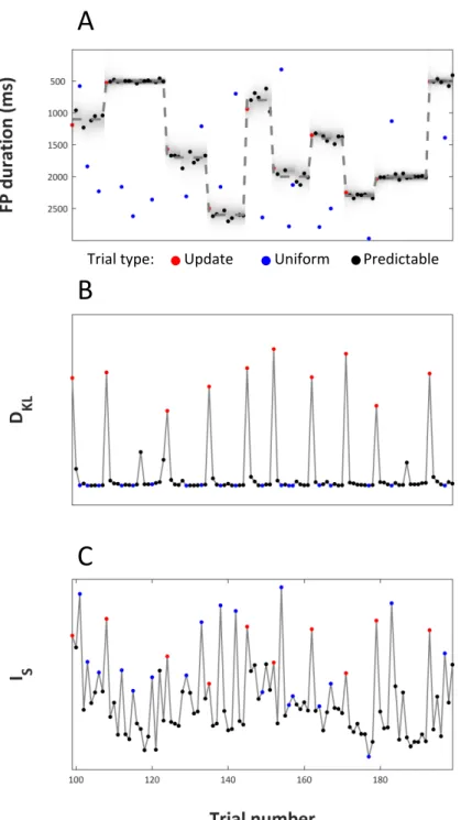
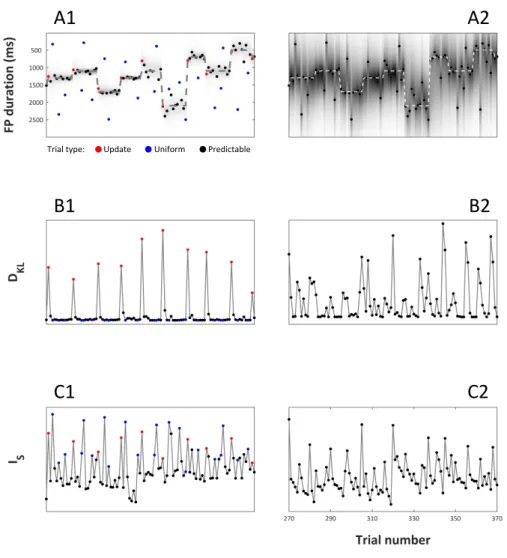
Figure 2.2 | Bayesian learner and model-based regressors. All panels show the data from 100 trials. Dot colors indicate trial types as reported in the legend. (A) Plot of the state of the normative Bayesian learner. On y axis is FP duration. The dashed line indicates the mean of the generative Gaussian distribution from which update and predictable foreperiods were drawn. Dots indicate the true FP duration on each trial. Shading indicates the estimated probability of FP duration given the prior, p(FP|prior). (B, C) Model-based regressors for updating (DKL)
and surprise (IS).
C
A
B
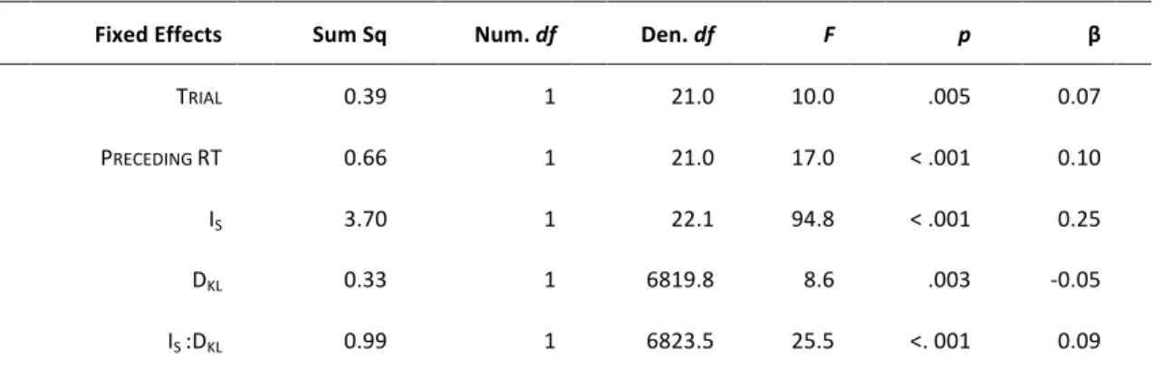
2.2.5 Behavioral data analysis
Data from error trials (with anticipated or without responses) and post-error trials were excluded from analysis. Reaction times (RTs) were log-transformed to mitigate the influence of non-normal distribution and skewed data. Following the procedure proposed by Baayen and Milin (2010), log-transformed RTs were analyzed by conducting Linear Mixed Models (LMM), using the lme4 library (Bates, Mächler, Bolker, & Walker, 2014) in R (R Core Team, 2015). In our main analysis, we investigated the behavioral correlates of surprise and updating by using IS and DKL as
regressors of interest. A full LMM was specified as follows: IS and DKL (and their
interaction) as well as TRIAL, that represents the rank-order of a trial, and log-RT at
the preceding trial (PRECEDING RT), were entered as fixed-effects predictors. The
random structure include correlated by-subject random intercepts and by-subject random slopes for TRIAL, PRECEDING RT, IS and DKL. All these continuous predictors
were standardized using Z-score in order to have the same scale, which allows comparing them statistically. The variables TRIAL andPRECEDING RT were included to
control for the temporal dependencies that usually occur between successive trials (Baayen & Milin, 2010). Specifically, TRIAL was included to capture possible effects of
learning and fatigue, while PRECEDING RT was used to take into account the RT
autocorrelation between subsequent trials. Using the function step from the
lmerTest library (Kuznetsova, Brockhoff, & Christensen, 2015), a stepwise variable selection was performed starting from the full model to eliminate non-significant effects from the full LMM.
2.2.6 fMRI data analysis
Data acquisition. Structural and functional images were acquired using a 3T Ingenia Philips whole body scanner (Philips Medical Systems, Best, The Netherlands) equipped with a 32-channel head-coil, at the Neuroradiology Unit of the University Hospital of Padova, Italy. Functional data were obtained using a whole head T2-weighted echo-planar image (EPI) sequences (repetition time, TR: 2000 ms; echo time, TE: 30 ms; 39 axial slices with ascending acquisition; voxel size: 3 × 3 × 3 mm;
flip angle, FA: 76°; field of view, acquisition matrix: 84 × 84). Excluding the four dummy scans for stabilization of the T1-saturation effect, the functional acquisitions consisted of 8 minutes of resting state activity, which will not be discussed in this thesis, followed by a total of 39.4 minutes of task related activity. To correct fMRI images for spatial distortion, at the beginning of each of the six runs, two spin echo EPI images with reversed phase encoding directions were acquired. These images are geometrically matched (same field of view and voxel size) with the functional images (Glasser et al., 2013). After functional session, high resolution T1- and T2- weighted anatomical images (T1w: TR/TE: 8.10/3.72 ms; 180 sagittal slices; FA: 8°; voxel size: 1 × 1 × 1 mm; acquisition matrix: 256 × 256; T2w: TR/TE: 2500/249 ms; 180 sagittal slices; FA: 90°; voxel size: 0.97 × 0.97 × 1 mm; acquisition matrix: 256 × 256) were collected. In order to avoid head movement during scanning, small foam cushions and sponge pads were placed around the participant’s head. Subjects also wore earplugs to reduce acoustic noise.
MRI preprocessing. First,spatial distortion of functional data were corrected using the susceptibility-induced off-resonance field estimated from the two oppositely phase-encoded spin echo EPI images as implemented in the FSL (FMRIB Software Library, version 5.0.7) toolbox “topup” (Andersson, Skare, & Ashburner, 2003; S. M. Smith et al., 2004). This step improves the following coregistration step between fMRI and structural image (Glasser et al., 2013). Functional data were then slice-timing corrected using the middle slice as the reference frame, rigidly realigned to the first volume and spatially smoothed using a Gaussian kernel with a full-width at half-maximum (FWHM) of 5 mm using SPM12 (Statistical Parametric Mapping software; Wellcome Department of Cognitive Neurology, London, UK; http://www.fil.ion.ucl.ac.uk/spm). Participant’s head movements were quantified by means of framewise displacement (FD) index which represents the sum of the absolute values of the derivatives of the translational and rotational realignment parameters (Power, Barnes, Snyder, Schlaggar, & Petersen, 2012). Subjects with mean FD above two standard deviations from the mean of all subjects (group mean = 0.09 mm, standard deviation = 0.02 mm) were excluded. The deformation field that mapped the individual functional data to standard Montreal Neurological
Institute (MNI) template was derived combining several steps, all implemented with FSL (Jenkinson, Beckmann, Behrens, Woolrich, & Smith, 2012; S. M. Smith et al., 2004). Usually a typical workflow involves the coregistration of the functional image to the T1-weighted anatomical image and the warp of the structural image to a template. Here, a T2-weighted anatomical image was used as an intermediate target since it has the same acquisition modality of fMRI data, but the same high-resolution with clear region boundary contours of T1-weighted anatomical images. First, T1-weighted anatomical image was bias-field corrected and a non-linear transformation to MNI template was estimated (T1>MNI). Both T2- and T1- weighted structural images were skull-stripped and then a 6-parameter transformation from the former to the latter was computed (T2>T1). At the end, a 12-parameter affine transformation from the first volume of the functional data to the T2-weighted skull-stripped anatomical image was estimated (fMRI>T2) and combined with the T2>T1 and T1>MNI transformations. The resulting transformation was then used to map the results obtained at individual level in the functional space to the MNI template.
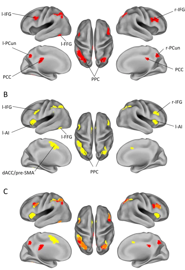
Whole-brain analysis. Statistical analyses were carried out using SPM12 (Ashburner et al., 2014) to identify the volumes of interest (VOIs) for the functional connectivity (FC) analysis. For each participant, first-level analysis was performed into the subject space (i.e. not normalized) using two general linear models (GLMs). For each GLM, the task was modeled with three regressors that were the main effect of the FP, the main effect of target onset, and either DKL or IS, estimates of head
movements were also included as six additional regressors of no interest. Slow signal drifts were removed using a 128 s high-pass filter. The main effect of the foreperiod was model as a boxcar starting from the cue onset and with duration equal to the FP length. The main effect of target onset was modeled as a delta function at the target onset modulated by the model-based regressor, DKL or IS, respectively. All these
regressors were convolved with the hemodynamic response function. As in the behavioral analysis, these two parametric modulators (PMs) were standardized using Z-score and orthogonalized with regard to target onset. The decision of running two GLMs instead of a single GLM including both PMs was made to keep variance that these two PMs likely share. Since this analysis was preliminary to FC, keeping this
shared variance is important to obtain a more exhaustive picture of the networks involved in processing and differentiating surprising information1. For each participant and each GLM, a t-contrast was computed for each PM versus zero (i.e. baseline). At the group level, individual participants’ Z-statistic maps were normalized to MNI template as described in the previous section. Then, for each GLM, group-level maps were generated with random-effect models using participants’ contrast maps. Group statistics were assessed for cluster-wise significance using a cluster-defining threshold of p < .001 and a cluster significance threshold of p < .05 (FWE-corrected). Furthermore, a third GLM with the hazard rate of the target onset (i.e. h(FPonset)) as PM was run in order to replicate previous
findings on hazard rate (Bueti et al., 2010).
Functional connectivity analysis. Task-related functional connectivity analysis was computed using the correlational psychophysiological interaction (cPPI) toolbox (Fornito, Harrison, Zalesky, & Simons, 2012). In classical PPI analyses (Friston et al., 1997), the activity time course from a specific seed region is extracted and multiplied by a task regressor of interest to isolate task-specific modulations in the functional coupling between the seed region and other brain regions. This approach is regression-based, in the sense that for each pair of time series the seed region activity is used as a predictor of the activity in the other regions. This implies that PPI is a form of effective connectivity (Friston et al., 1997), thus, it is suitable when there are clear hypotheses about which region may modulate activity in other regions (Fornito et al., 2012). Since we had no such specific predictions, we employed the cPPI approach, which provides a measure of functional connectivity that does not require directional assumptions. Briefly, for any given pair of brain regions their time course is multiplied by the task-regressor to obtain two PPI terms. Then, the partial correlation between the two PPI terms is estimated while controlling for possible confounds (e.g., task-unrelated connectivity, noise). In a nutshell, starting from a set of regions the cPPI analysis returns a functional connectivity matrix of pair-wise covariations in task-specific modulations of neural activity. We estimated two cPPI correlation matrices, one for each of the two model-based regressors, DKL and IS. For