AIS Electronic Library (AISeL)
WHICEB 2016 Proceedings
Wuhan International Conference on e-Business
Summer 5-27-2016
Solving Vehicle Routing Problem in the Logistics
Distribution Based on Immune Genetic Algorithm
Xuebing Bo
School of Economics and Management, Xidian University, Xi’an, 710017, China, [email protected]
Hui Li
School of Economics and Management, Xidian University, Xi’an, 710017, China, [email protected]
Follow this and additional works at:
http://aisel.aisnet.org/whiceb2016
This material is brought to you by the Wuhan International Conference on e-Business at AIS Electronic Library (AISeL). It has been accepted for inclusion in WHICEB 2016 Proceedings by an authorized administrator of AIS Electronic Library (AISeL). For more information, please contact
Recommended Citation
Bo, Xuebing and Li, Hui, "Solving Vehicle Routing Problem in the Logistics Distribution Based on Immune Genetic Algorithm" (2016).WHICEB 2016 Proceedings. 23.
Solving Vehicle Routing Problem in the Logistics Distribution Based
on Immune Genetic Algorithm
Xuebing Bo1, Hui Li2*
1
School of Economics and Management, Xidian University, Xi’an, 710017, China
2
School of Economics and Management, Xidian University, Xi’an, 710017, China
Abstract: In logistic transport industry, individual demands and diversity requirements are matters in transport operation; this paper focused on solving vehicle routing problem (VRP) by using the immune genetic algorithm (IGA). In this algorithm, firstly, establish the mathematical model of VRP. Secondly, design the IGA of which use natural number coding method to encode antibodies; apply R continuous method to calculate the affinity between antibodies; use the roulette wheel selection method to select good individuals; adopt partial matching method to improve the crossover operation; use simple inversion mutation method for mutation operation. Finally, example analysis proves that using the IGA can find out the optimal path quickly and efficiently.
Keywords: model, immune genetic algorithm, vrp, example analysis
1. INTRODUCTION
In today's era of electronic commerce, the global logistics industry has a new development trend. The core aim of modern logistics service is meeting the needs of customers with the minimum comprehensive cost. And in many factors of reducing the logistics cost, the proportion of distribution costs is particularly prominent. Thus, vehicle routing optimization is still a hot research topic in the field of logistics.
Currently, the research methods of VRP mainly include accurate algorithm, heuristic algorithm and intelligent optimization algorithms. Such as, Chunyu Ren and Shiwei Li [1] have designed a new genetic algorithm to solve the VRP. Baozhen Yao [2] has found the optimal path of VRP, quickly and efficiently, with the improved particle swarm algorithm; Ulrich Derigs [3] has applied hybrid heuristic algorithm to solve the complicated nonlinear VRP, Jianru Zheng [4] has introduced the improved particle swarm optimization algorithm in detail, simulated the VRP and found out the optimal path; In matlab environment, using the genetic algorithm is proposed by Xiuhong Guo [5] for VRP with optimal solutions, effectively reduce the transportation cost of distribution. Huayu Shi [6] has proposed the improved ant colony algorithm to shorten the total distance of vehicle distribution, optimized the logistics distribution vehicle routing, and reduced the transportation cost. According to the mathematical model of logistics distribution VRP and specific feature, Xiangli Ma and Huizhen Zhang [7] has designed bat algorithm for solving VRP problems, and verified the effectiveness and feasibility of the bat algorithm for solving VRP through simulation examples and comparison with particle swarm optimization (PSO) algorithm. In vehicle routing problem, however, IGA is used rarely. In the design of IGA, the calculation of the affinity between antibody and antibody is often the way of information entropy, which makes the computation complexity increase. So, in this paper, in the matlab environment, IGA is designed with R continuous method to calculate the affinity of antibodies that the calculation process is simplified, and compared with genetic algorithm, the immune genetic algorithm is proved to be able to solve the VRP, quickly and efficiently, by the example analysis.
*
2. MATHEMATICAL MODEL OF VRP IN LOGISTICS DISTRIBUTION
In logistics distribution, the objective of VRP is to arrange several vehicles to a lot of customers from the distribution center and return to the common distribution center without exceeding the capacity of each vehicle at minimum cost. Each customer's geographical position and demand and the loading capacity of every vehicle must be certain. It requires a reasonable planning of vehicle routing so that the total transport distance is the shortest, and that meets the following conditions:
(1)The sum of customers’ demands on the each path is less than the capacity of a vehicle;
(2)The total distance of each distribution path is less than the maximum transport distance of a vehicle; (3)Meet the needs of each customer, and each customer’s demands can only be distributed by a vehicle; (4)The amount of transport is proportional to the cost;
(5)The number of vehicles in the distribution center, the capacity and the maximum transport distance of each vehicle, the number of customers, the demands of each customer and the transportation distance between the distribution center with the customers are all known constants.
VRP mathematical model [5] [8] of logistics distribution is established by reference [5] and [8] and taking the constraints and optimization of VRP in the logistics distribution into account.
Hypothesis that there are k vehicles in the distribution center, the loading capacity of vehicle k is k
Q (k=1, 2, ...,K), and the maximum transport distance of a distribution is Dk, need to deliver to L
customers, customer i s' demand amount is qi(i=1, 2, ...,L), the linear distance from customer i to customer j is dij , the distance from the distribution center to customer j is d0j(i j, =1, 2, ...,L ); Hypothesis that the number of customers distributed by vehicle k is nk(nk =0shows the vehicle k is not involved in distribution), Rkshows the customers’ aggregation in path k, and the element rkishows the sequence of customer rki is i in path k, which does not include the distribution center. Hypothesis that
0 0
k
r = shows the distribution center, then the VRP model can be established as follows: ( 1) 0 1 1 Min ( ) k k i ki knkk n K r r r r k k i Z d − d sign n = =
⎡
⎤
=
⎢
+
∗
⎥
⎣
⎦
∑ ∑
(1) Constraints:s t
. .
1 k ki n r k i q Q =≤
∑
(2) ( 1) 0 1( )
k k i ki knk k n r r r r k k i d − d sign n D =+
∗
≤
∑
(3) 0≤nk ≤L (4) 1 K k k n L ==
∑
(5) Rk ={
r rki ki∈{
1, 2, 3, ...,L}
,i=1, 2, 3, ...nk}
(6) Rk1∩Rk2 = ∅ ∀ ≠k1 k2 (7) ( ) 1, 1 0, k k n sign n other ≥ =⎧
⎨
⎩
(8)In the above VRP mathematical model of logistics distribution, formula (1) is the objective function; formula (2) shows the sum of customers’ demands on the each distribution path is less than the loading capacity of a vehicle; formula (3) shows the total distance of each distribution path is less than the maximum transport distance of a vehicle; formula (4) shows the number of customers in each path is less than the total number of
customers; formula (5) shows each customer obtains the distribution; formula (6) is the set of customers in each path; formula (7) ensures that each customer’s demands can only be fulfilled once by one vehicle; formula (8) shows if the number of customers distributed by vehicle k is more than 1, the vehicle k takes part in the distribution and sign n( )k =1, or the vehicle k does not take part in the distribution and sign n( )k =0.
3. SOLVING VRP WITH IMMUNE GENETIC ALGRITHM 3.1 Introduction of immune genetic algorithm
Immune genetic algorithm is a kind of improved genetic algorithm based on biological immune system, which antigen corresponds to the objective function for solving practical problems, and the antibody corresponds to the solution of actual problem. This algorithm is a new optimization combination method which is based on the genetic algorithm and the learning, adaptability and memory function and other characteristics of the biological immune system. This algorithm finds a broader space for complex problems.
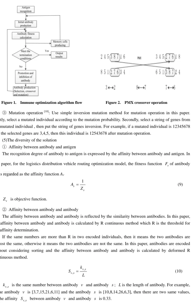
3.2 Immune genetic algorithm for VRP in logistics distribution Immune genetic algorithm flow chart [9] is shown in figure 1. Specific methods and steps of immune genetic algorithm: (1)Antibody-encoding
According to the characteristics of logistics distribution VRP, this paper uses a simple natural number coding method to encode antibody. First, generate the non repetition natural number 1,2,…,M,M+1,…,M+K-1 which 0 denotes the distribution center, 1,2,…,M denote customers and K denotes the total number of vehicles, then permutate the M+K-1 numbers randomly to form an individual. For example, if there are 2 vehicles to 8 customers for delivery, it generates the natural number1,2,…,9 which 9 denotes the distribution center and permutates the 9 numbers to form a logistics distribution path. The individual 126398547 represents there are 2 distribution paths which one is 0-1-2-6-3-9 (0) and the other is 9 (0)-8-5-4-7-0.
(2)Generation of initial population
If the memory is not empty, the initial antibody population is selected from the memory database, otherwise, it will be generated by the feasible solution space. Antibody memory function is an important characteristic of immune optimization algorithm, and the system can keep some better individuals after solving a problem. When each generation of antibody updates, the optimal m antibodies are retained in the memory database and compared with the existing antibodies in its memory, then replace the poor antibodies.
(3)Fitness calculation of antibody.
If the distribution path corresponding to the antibody v is feasible, the fitness value of the antibody v is 1
v v
F Z
= , otherwise the fitness value is v 1
(
)
vF
Z α
=
+ ,α which is overweight value is 4000 in this paper.
(4)Immune operation
① Selection operation: Adopt the roulette wheel selection method to select antibody. The selected probability of antibody v is expectation reproduction rate calculated by the formula (12).
② Crossover operation: In this paper, a partial matching method (PMX) is used for crossover operation. Randomly select two chromosomes in father generation. Take father (2 4 5 3 8 7 1 6) and father (8 5 1 2 7 6 3 4) for example: first, select two crossing points randomly, then the numbers between the two points are crossed, and the other numbers are replaced by the matching number or the copy. In this example, assuming the position of the first crossing point is 4, and the position of the second crossing point is 6, then 3, 8, 7 are selected in the father 1 and 2, 7, 6 are selected in the father 2, so 3 matches with 2, 8 matches with 7, 7 matches with 6. The matching process is shown in figure 2.
Figure 1. Immune optimization algorithm flow Figure 2. PMX crossover operation
③ Mutation operation [10]: Use simple inversion mutation method for mutation operation in this paper. Firstly, select a mutated individual according to the mutation probability. Secondly, select a string of genes from the mutated individual , then put the string of genes inversion. For example, if a mutated individual is 12345678 and the selected genes are 3,4,5, then this individual is 12543678 after mutation operation.
(5)The diversity of the solution
① Affinity between antibody and antigen
The recognition degree of antibody to antigen is expressed by the affinity between antibody and antigen. In this paper, for the logistics distribution vehicle routing optimization model, the fitness function Fvof antibody
v is regarded as the affinity function AV
1 v v A Z = (9) v Z is objective function.
② Affinity between antibody and antibody
The affinity between antibody and antibody is reflected by the similarity between antibodies. In this paper, the affinity between antibody and antibody is calculated by R continuous method which R is the threshold for the affinity determination.
If the same numbers are more than R in two encoded individuals, then it means the two antibodies are almost the same, otherwise it means the two antibodies are not the same. In this paper, antibodies are encoded without considering sorting and the affinity between antibody and antibody is calculated by deformed R continuous method. Sv s, kv s, L = (10) , v s
k is the same number between antibody v and antibody s; Lis the length of antibody. For example, if the antibody v is [3,7,15,21,6,11] and the antibody s is [10,8,14,26,6,3], then there are two same values, so the affinity Sv s, between antibody v and antibody s is 0.33.
③ Antibody concentration
The antibody concentration Cv is the proportion of similar antibodies in the population.
,
1
v v s i N C S N ∈=
∑
(11)N is the total number of antibody. , 1, , 0, v s v s S T S else > =
⎧
⎨
⎩
; In this paper, Twhich is a preset threshold is 0.9.④ Expectation reproduction probability
In population, the expectation reproduction probability of each individual is decided by the affinity Av
between antibody and antigen and the concentration Cv of antibody. v
(
1
)
v v vZ
C
p
Z
C
α
α
=
+ −
∑
∑
(12) In this paper, αwhich is constant is 0.95.The formula (12) shows that the higher the affinity, the higher the expectation reproduction probability and the higher the concentration, the lower the expectation reproduction probability. This is not only to promote the high affinity antibodies, but also inhibit the high concentrations antibodies, so as to ensure the diversity of antibodies.
4. EXAMPLE ANALYSIS
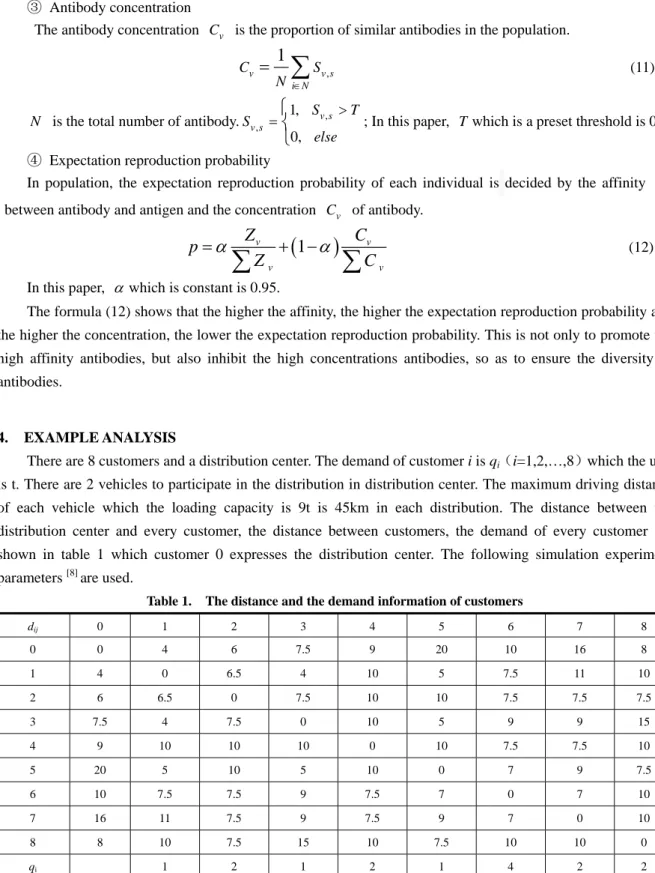
There are 8 customers and a distribution center. The demand of customer i is qi(i=1,2,…,8)which the unit
is t. There are 2 vehicles to participate in the distribution in distribution center. The maximum driving distance of each vehicle which the loading capacity is 9t is 45km in each distribution. The distance between the distribution center and every customer, the distance between customers, the demand of every customer are shown in table 1 which customer 0 expresses the distribution center. The following simulation experiment parameters [8] are used.
Table 1. The distance and the demand information of customers
dij 0 1 2 3 4 5 6 7 8 0 0 4 6 7.5 9 20 10 16 8 1 4 0 6.5 4 10 5 7.5 11 10 2 6 6.5 0 7.5 10 10 7.5 7.5 7.5 3 7.5 4 7.5 0 10 5 9 9 15 4 9 10 10 10 0 10 7.5 7.5 10 5 20 5 10 5 10 0 7 9 7.5 6 10 7.5 7.5 9 7.5 7 0 7 10 7 16 11 7.5 9 7.5 9 7 0 10 8 8 10 7.5 15 10 7.5 10 10 0 qi 1 2 1 2 1 4 2 2
The population size is 50, the encoding length is 9, the crossover probability is 0.95, the mutation probability is 0.05, and the diversity evaluation parameter is 0.95.
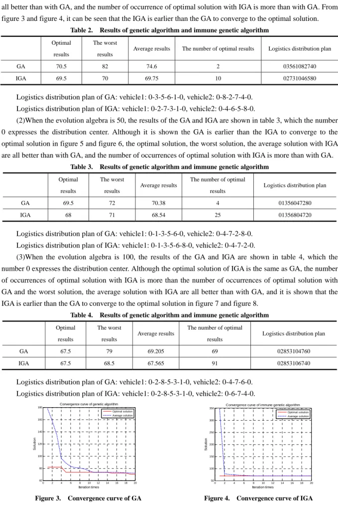
When the evolution algebra is 20, 50 and 100 respectively, the results of the GA and IGA are shown in table 2, table 3 and table 4. And the convergences of the solution are shown in figure 3, figure 4, figure 5, figure 6, figure 7 and figure 8.
0 expresses the distribution center. The optimal solution, the worst solution, the average solution with IGA are all better than with GA, and the number of occurrence of optimal solution with IGA is more than with GA. From figure 3 and figure 4, it can be seen that the IGA is earlier than the GA to converge to the optimal solution.
Table 2. Results of genetic algorithm and immune genetic algorithm Optimal
results
The worst results
Average results The number of optimal results Logistics distribution plan
GA 70.5 82 74.6 2 03561082740
IGA 69.5 70 69.75 10 02731046580
Logistics distribution plan of GA: vehicle1: 0-3-5-6-1-0, vehicle2: 0-8-2-7-4-0. Logistics distribution plan of IGA: vehicle1: 0-2-7-3-1-0, vehicle2: 0-4-6-5-8-0.
(2)When the evolution algebra is 50, the results of the GA and IGA are shown in table 3, which the number 0 expresses the distribution center. Although it is shown the GA is earlier than the IGA to converge to the optimal solution in figure 5 and figure 6, the optimal solution, the worst solution, the average solution with IGA are all better than with GA, and the number of occurrences of optimal solution with IGA is more than with GA.
Table 3. Results of genetic algorithm and immune genetic algorithm Optimal
results
The worst results
Average results The number of optimal
results
Logistics distribution plan
GA 69.5 72 70.38 4 01356047280
IGA 68 71 68.54 25 01356804720
Logistics distribution plan of GA: vehicle1: 0-1-3-5-6-0, vehicle2: 0-4-7-2-8-0. Logistics distribution plan of IGA: vehicle1: 0-1-3-5-6-8-0, vehicle2: 0-4-7-2-0.
(3)When the evolution algebra is 100, the results of the GA and IGA are shown in table 4, which the number 0 expresses the distribution center. Although the optimal solution of IGA is the same as GA, the number of occurrences of optimal solution with IGA is more than the number of occurrences of optimal solution with GA and the worst solution, the average solution with IGA are all better than with GA, and it is shown that the IGA is earlier than the GA to converge to the optimal solution in figure 7 and figure 8.
Table 4. Results of genetic algorithm and immune genetic algorithm Optimal
results
The worst
results Average results
The number of optimal
results Logistics distribution plan
GA 67.5 79 69.205 69 02853104760
IGA 67.5 68.5 67.565 91 02853106740
Logistics distribution plan of GA: vehicle1: 0-2-8-5-3-1-0, vehicle2: 0-4-7-6-0. Logistics distribution plan of IGA: vehicle1: 0-2-8-5-3-1-0, vehicle2: 0-6-7-4-0.
0 2 4 6 8 10 12 14 16 18 20 60 80 100 120 140 160 180 Iteration times So lu ti o n
Convergence curve of genetic algorithm
Optimal solution Average solution 0 2 4 6 8 10 12 14 16 18 20 50 100 150 200 250 300 350 Iteration times Sol u ti on
Convergence curve of immune genetic algorithm
Optimal solution Average solution
0 5 10 15 20 25 30 35 40 45 50 60 80 100 120 140 160 180 200 Iteration times Sol u ti o n
Convergence curve of genetic algorithm
Optimal solution Average solution 0 5 10 15 20 25 30 35 40 45 50 60 80 100 120 140 160 180 200 220 Iteration times So lu ti o n
Convergence curve of immune genetic algorithm
Optimal solution Average solution
Figure5. Convergence curve of GA Figure 6. Convergence curve of IGA
0 10 20 30 40 50 60 70 80 90 100 60 80 100 120 140 160 180 Iteration times So lu ti o n
Convergence curve of genetic algorithm
Optimal solution Average solution 0 10 20 30 40 50 60 70 80 90 100 50 100 150 200 250 300 350 400 450 Iteration times So lu ti o n
Convergence curve of immune genetic algorithm
Optimal solution Average solution
Figure7. Convergence curve of GA Figure 8. Convergence curve of IGA
From table 2, table 3 and table 4, it can be seen whatever the evolution algebra is, the optimal solution, the worst solution, the average solution with IGA are all better than with GA, and the number of occurrence of optimal solution with IGA is more than with GA. It is shown that the IGA is earlier than the GA to converge to the optimal solution in figure 3 and figure 4, figure 7 and figure 8. So IGA is superior to GA in vehicle routing problem.
5. CONCLUSIONS
Based on example analysis, the IGA is more quickly and efficiently than the GA to find the optimal solution that is the optimal path of logistics distribution, thus the total distance of logistics distribution is shortened, and the transportation cost is saved. At the same time, compared with the GA, the IGA has the following characteristics: it can maintain the diversity of antibodies and improve local search ability; it has the function of immune memory and self-adjustment and can accelerate the search speed, improve the global search ability, and avoid falling into local solution. Thus, it is more practical significance and value to reduce operating cost and improve economic benefit.
REFERENCES
[1] Chunyu Ren, Shiwei Li. (2012).New Genetic Algorithm for Capacitated Vehicle Routing Problem. Advances in Computer Science and Information Engineering, 168: 695-700.
[2] Baozhen Yao. (2015).An improved particle swarm optimization for carton heterogeneous vehicle routing problem with a collection depot. Annals of Operations Research, 1-18.
[3] Ulrich Derigs. (2014).Experience with a framework for developing heuristics for solving rich vehicle routing problems. Journal of Heuristics, 20(1): 75-106.
[4] Jianru Zheng. (2013).Research on Vehicle Routing Problem Based on Improved Particle Swarm Optimization Algorithm. Beijing: North China Electric Power.
[5] Xiuhong Guo. (2013).Research of Vehicle Routing Optimization Based on Genetic Algorithm. Sichuan ordnance Journal, (01): 94-96.
[6] Huayu Shi. (2012).The Application of the Improved Ant Colony Algorithm on Actual Vehicle Routing Problem [D]. Shandong: Shandong University.
[7] Ma Xiangli, Zhang Huizhen, Ma Liang. (2015). Application of bat algorithm in the optimization of logistics distribution vehicle routing problem. Mathematics in Practice and Theory, 45(24): 80-86.
[8] Yue Yu, Hongzhi Hu. (2009).Solving Logistics Distribution Routing Problem by An Improved Genetic Algorithm. Computer technology and development, (03): 52-54.
[9] Fei Gao. (2014).Super learning manual for MATLAB intelligent algorithm. Beijing: Peng Zhihuan & Yang Linjie, 275-289.
[10]Lijie Yuan. (2013).Immune Genetic Algorithm Used and Research on Vehicle Routing Problem. Dalian: Dalian Maritime University.