Global Optimization Strategies for Two-Mode
Clustering
∗
Joost van Rosmalen
†Patrick J.F. Groenen
†Javier Trejos
‡William Castillo
‡October 2005
Econometric Institute Report EI 2005-33
Abstract
Two-mode clustering is a relatively new form of clustering that clusters both rows and columns of a data matrix. To do so, a cri-terion similar to k-means is optimized. However, it is still unclear which optimization method should be used to perform two-mode clus-tering, as various methods may lead to non-global optima. This pa-per reviews and compares several optimization methods for two-mode clustering. Several known algorithms are discussed and a new, fuzzy algorithm is introduced. The meta-heuristics Multistart, Simulated Annealing, and Tabu Search are used in combination with these al-gorithms. The new, fuzzy algorithm is based on the fuzzy c-means algorithm of Bezdek (1981) and the Fuzzy Steps approach to avoid local minima of Heiser and Groenen (1997) and Groenen and Jajuga (2001). The performance of all methods is compared in a large sim-ulation study. It is found that using a Multistart meta-heuristic in combination with a two-mode k-means algorithm or the fuzzy algo-rithm often gives the best results. Finally, an empirical data set is used to give a practical example of two-mode clustering.
Key words: Two-mode clustering, algorithms, fuzzy clustering, simu-lation, simulated annealing, tabu search, multistart.
∗We would like to thank Peter Verhoef for kindly providing the data used in this paper. †Econometric Institute, Erasmus University Rotterdam, P.O. Box 1738, 3000 DR
Rot-terdam, The Netherlands, e-mail: [email protected]
1
Introduction
Clustering can be seen as one of the cornerstones of classification. In this paper, we limit ourselves to clustering into partitions of objects. Consider a typical two-way two-mode data set of respondents by variables. Often, clus-tering algorithms are applied to just one mode of the data matrix, which can be done in a hierarchical or non-hierarchical way. Among the non-hierarchical methods,k-means clustering (Hartigan, 1975) is one of the most popular non-hierarchical methods. Moreover, it has the advantage of a loss function being optimized.
A relatively new form of clustering is two-mode clustering. In two-mode clustering, both rows and columns of a two-mode data matrix are assigned to clusters. Each row of a two-mode data matrix is assigned to a row cluster, and each column to a column cluster. Elements of the data matrix which are both in the same row cluster and in the same column cluster should be close. DeSarbo (1982) described such a two-mode clustering method, called the GENNCLUS model. Another form of two-mode clustering is blockmodeling, which is often used in social network analysis (see, for example, Noma and Smith, 1985). An extensive overview of two-mode clustering methods can be found in Van Mechelen, Bock, and De Boeck (2004).
In this article, we focus on partitioning the sets of rows and columns using a least-squares criterion that models the elements of the data matrix belong-ing to the same row and column cluster by their average. Several optimiza-tion methods for finding the optimal partioptimiza-tioning for two-mode clustering are known from the literature. However, these methods are not guaranteed to find the global optimum and often get stuck in local minima. Therefore, we study the local minimum problem of two-mode clustering. In addition, a new optimization method for two-mode clustering is introduced, based on the fuzzy c-means algorithm of Bezdek (1981). Here, we review and com-pare these optimization methods. By a simulation study, we identify the methods that perform well under most circumstances, within a reasonable computational effort. All methods are based on meta-heuristics that aim to find globally optimal solutions in an acceptable amount of CPU time. In our comparisons we use both simulated and empirical data.
The remainder of this article is organized as follows. In Section 2, we introduce the notation and give an overview of the optimization problem, including two local search algorithms. Section 3 describes the implementation of threemeta-heuristicsfor two-mode clustering, which also uses the two local search algorithms. In Section 4, we introduce the fuzzy two-mode clustering method and give some theoretical background behind this method. In Section 5, we compare the performance of the methods using an extensive simulation
study. Section 6 uses an empirical data set to compare the methods and to give a practical example of two-mode clustering. Finally, we draw conclusions and give recommendations for further research.
2
Overview of Optimization Problem
To define the two-mode clustering problem, consider the following notation:
Xn×m = (xij)n×m Two-mode data matrix of n rows and m columns.
Pn×K = (pik)n×K Cluster membership matrix of the rows with K the
number of row clusters, andpik = 1 if row i belongs
to row clusterk, and pik = 0 otherwise.
Qm×L= (qjl)m×L Cluster membership matrix of the columns with L
the number of column clusters, andqjl= 1 if column
j belongs to column cluster l, and qjl = 0 otherwise.
VK×L= (vkl)K×L Matrix with cluster centers for row clusterk and
col-umn clusterl.
En×m = (eij)n×m Matrix with errors from cluster centers.
Usually, the rows (the first mode) of X correspond to objects, and the columns (the second mode) ofXrefer to variables. The elements ofXcan be associations, confusions, fluctuations, etc., between row and column objects. It only makes sense to apply to two-mode clustering if the values in the data matrix can be compared amongst each other. Therefore, if one of the modes refers to variables, the values among the variables must be comparable, stan-dardized, or measured on the same scale. In the remainder of this paper, we assume that this condition is satisfied by the data.
Two-mode clustering assigns each element of X to a row cluster and a column cluster. If L equals m, every column can be placed in a cluster by itself, so that two-mode clustering reduces to one-mode k-means clustering, and the same is true if K = n. The matrix V can be interpreted as the combined cluster means. The cluster memberships are given by the matrices
P and Q. Together, these three matrices P, Q, and V approximate the information in X by PVQ0. To make this approximation as close to X as possible, we use the additive model
X=PVQ0+E, (1)
where E is the error of the model.
Two-mode clustering searches for the optimal partitionP, Q and cluster centers V that minimize the sums of squares of E. This objective amounts to minimizing the squared Euclidean distance of the data points to their
respective clusters centers in V. Therefore, the criterion to be minimized can be expressed as f(P,Q,V) =kX−PVQ0k2 = K X k=1 L X l=1 n X i=1 m X j=1 pikqjl(xij −vkl)2. (2)
It is not required to use the Euclidean metric; other metrics have been used as well, especially in one-mode clustering (see, for example, Bock, 1974). However, in this study, we restrict ourselves to the Euclidean metric. The optimal cluster membership matrices must satisfy the following constraints. 1. The cluster memberships of each row and column object must sum to
one, so that PK
k=1pik = 1 and
PL
l=1qjl= 1.
2. All cluster membership values must be either zero or one, thus pik ∈
{0,1}and qjl ∈ {0,1}.
3. None of the row or column clusters is empty, that is Pn
i=1pik >0 and
Pm
j=1qjl>0.
The first two constraints require that each row of P and Q contains exactly one element with the value 1. Hence, each row and column object is assigned to exactly one cluster. These two constraints are necessary and sufficient for the second equality in (2) to hold. A partition that violates the third constraint cannot be optimal according to (2), so, in principle, the third constraint is not required during the estimation. However, some algorithms may lead to a partition with empty clusters. Therefore, we adapt these algorithms to correct for potential empty clusters or prevent them from happening.
No polynomial time algorithm is known for the global minimization of f(P,Q,V). Even for small n and m, the number of possible partitions can become extremely large and a complete enumeration of the possible solutions is almost always computationally infeasible. However, when two of the three matrices P, Q, and V are known, the optimal value of the third matrix can be computed quite easily. When both P and Q are known, the optimal cluster centers V can be computed as
vkl = Pn i=1 Pm j=1pikqjlxij Pn i=1 Pm j=1pikqjl , (3)
which is simply the average of the elements of X belonging to row clusterk and column cluster l. When V and either P or Q are known, the problem
of minimizing f(P,Q,V) becomes a linear program. As this linear program is particularly simple, its solution can be given in a closed form expression. When V and Q are known, the optimal value of P can be computed as follows. Let cik = Pm j=1 PL l=1qjl(xij −vkl)2. Then, pik = 1 if cik = min1≤r≤Kcir, 0 otherwise. (4)
When P and V are known, the optimal matrix Q can be computed in a similar fashion.
A number of algorithms for finding an optimal two-mode partition have been proposed in the literature. Two of these algorithms are discussed in the remainder of this section. Both algorithms are deterministic and perform a local search of the solution space. In the next section, we will discuss methods that adapt these local search algorithms to perform global optimization.
2.1
Alternating Exchanges
The Alternating Exchanges algorithm was introduced by Gaul and Schader (1996). It tries to improve an initial partition by making a transfer of either a row or a column object and immediately recalculating V. The advantage of this approach is that updates can be obtained relatively fast. It performs the following steps:
1. Choose initial P and Q, and calculate V according to (3).
2. Repeat the following, until there is no improvement of f(P,Q,V) in either step.
(a) For eachi, k, transfer row object ito row class k and re-calculate
V according to (3). Accept the transfer if it has improved f(P,Q,V), otherwise return to the old Pand V.
(b) For each j, l, transfer column object j to column class l and re-calculateVaccording to (3). Accept the transfer if it has improved f(P,Q,V), otherwise return to the old Q and V.
The Alternating Exchanges algorithm always converges to a local mini-mum, as it decreases the value of f(P,Q,V) in every iteration, it is defined on a finite set, and f(P,Q,V) is bounded from below by 0.
2.2
Two-mode
k
-Means
Thek-means algorithm (Hartigan, 1975) is used frequently in one-mode clus-tering. It is one of the simplest and fastest ways to obtain a good partition, which accounts for its popularity in one-mode clustering. In addition, it can easily be extended to handle two-mode clustering. The so-called two-mode
k-means algorithm tries to improve an initial partition using (3) and (4). It consists of the following steps.
1. Choose initial P and Q.
2. Repeat the following, until there is no improvement of f(P,Q,V) in any step.
(a) UpdateV according to (3). (b) Letcik =
Pm
j=1
PL
l=1qjl(xij −vkl)2. Then update Paccording to
pik = 1 if cik = min1≤r≤Kcir, 0 otherwise. (5) (c) UpdateV according to (3). (d) Letdjl = Pn i=1 PK
k=1pij(xij −vkl)2. Then update Q according to
qjl=
1 if djl = min1≤r≤Ldjr,
0 otherwise. (6)
The two-mode k-means algorithm will always converge to a local opti-mum, as the value of the criterion f(P,Q,V) cannot increase in any step. However, it can happen that one or more clusters become empty after Step 2b or 2d. This situation is immediately corrected by transferring the row or column object with the highest value of PK
k=1pikcik or
PL
l=1qjldjl to the
empty cluster. As this transfer always improves the value of the criterion, the algorithm will still converge.
3
Meta-Heuristics for Global Optimization
The two algorithms introduced in the previous section only attempt to find locally optimal partitions. As no known polynomial time algorithm is capable of finding the global optimum in every instance, we revert to meta-heuristics
instead. These methods indeed aim for global optima but are not guaranteed to find them. In this section, we discuss the use of the three meta-heuristics
Multistart, Simulated Annealing, and Tabu Search. By combining these with the two local search algorithms (Alternating Exchanges and two-mode
k-means), we obtain four stochastic global optimization methods. The Fuzzy Steps method, which uses the Multistart heuristic, is introduced in the next section. Other algorithms and meta-heuristics have also been used for two-mode clustering. Hansohm (2001) used the genetic algorithm, but found it does not perform as well in two-mode clustering as it does in one-mode clustering. Gaul and Schader (1996) implemented a penalty algorithm, but concluded that it does not compare favorably with the Alternating Exchanges algorithm.
3.1
Multistart
The most simple heuristic is Multistart, which performs a given number of repetitions of a certain algorithm with random starting values in every repetition. The best result out of all repetitions is the final result of the Multistart heuristic. This method prevents the algorithm from incidentally reaching very bad solutions. Also, the Multistart heuristic will always find the global optimum if the number of repetitions is large enough. However, it depends on the function and the data how large the number of repetitions needs to be. In our case, the number of repetitions becomes prohibitively large to be able to guarantee a global minimum. However, even with a reasonable number of repetitions, Multistart often performs well.
We apply the Multistart heuristic to the Alternating Exchanges and the two-mode k-means algorithms described in the previous section. The initial partitions of the resulting optimization methods were chosen by randomly assigning each row and column object to a cluster, with uniform probability.
3.2
Simulated Annealing
Simulated Annealing is a meta-heuristic that simulates the slow cooling of a physical system. Similar to Alternating Exchanges, Simulated Annealing also performs a local search. However, to avoid getting stuck in local minima, Simulated Annealing also accepts, with a positive probability, transitions that increasef(P,Q,V); see Laarhoven and Aarts (1987) for more details on the Simulated Annealing meta-heuristic. Trejos and Castillo (2000) also applied Simulated Annealing in two-mode clustering.
The Simulated Annealing method uses as parameters a cooling rateγ <1 and the number of iterations r in which the temperature remains constant. It also chooses an initial value of the temperature T, and a maximum num-ber of iterations without accepted transitions, denoted by tmax. Simulated
Annealing consists of the following steps.
1. Choose initial P and Q and calculate V according to (3). 2. Choose the parametersr,γ, and a large, initial value ofT.
3. Repeat the following until there is no change in P and Q for the last tmax values of T.
(a) Do the followingr times:
i. Choose one of the two modes with equal probability.
ii. Choose one of the objects of this mode with uniform probabil-ity and transfer it to another cluster, also chosen with uniform probability.
iii. Update V according to (3) and calculate ∆f as the change in f(P, Q,V) achieved by the transfer and the subsequent updating ofV.
iv. Always accept the transfer if ∆f <0, otherwise accept it with probability exp(−∆f /T).
(b) SetT =γT.
The partition with the lowest value off(P,Q,V) found during estimation is retained as the final solution.
3.3
Tabu Search
The Tabu Search meta-heuristic was introduced by Glover (1986). Tabu Search also performs a local search, but tries to move away from local op-tima by maintaining a tabu list. The tabu list is a list of partitions that are temporarily not accepted. Here, we use the following method for Tabu Search in two-mode clustering, which is based on the Alternating Exchanges algorithm. Note that many other versions of Tabu Search are possible. We refer to Castillo and Trejos (2002) for a more detailed description of this method.
DefineZ(P,Q) = minVf(P,Q,V). The algorithm performs the
follow-ing steps.
1. Start with an initial partition (P,Q) and an empty tabu list.
2. Choose the number of iterations tmax and a maximum length of the
3. Perform the following stepstmax times.
(a) Generate a neighborhood of partitions N, consisting of the parti-tions that can be constructed by transferring one row or column object from (P,Q) to another cluster.
(b) Choose the partition (P,Q)cand as the partition in N with the
lowest value of Z(P,Q) that is not on the tabu list.
(c) Set (P,Q) = (P,Q)cand. If Z((P,Q)cand) < Z((P,Q)opt), then
(P,Q)opt = (P,Q)cand.
(d) Add (P,Q) to the tabu list. Remove the oldest item from the tabu list, if the list exceeds its maximum length.
The final solution of the algorithm is given by (P,Q)opt.
4
Fuzzy Two-Mode Clustering
Fuzzy methods relax the requirement that an object belongs to a single clus-ter, so that the cluster membership can be distributed over the clusters. For single mode clustering, the best known method is fuzzy c-means (Bezdek, 1981; for adaptations of this method see Groenen and Jajuga, 2001, and Tsao, Bezdek, and Pal, 1994). These methods try to make the optimization task easier by allowing for cluster membership values between 0 and 1. Here, we extend single mode fuzzy algorithms to the two-mode case. Below, we in-troduce a fuzzy two-mode clustering criterion. Section 4.1 gives an algorithm for finding an optimal fuzzy partition, based on Bezdek (1981). Section 4.2 describes the Fuzzy Steps method, that reduces the fuzziness of the solution in steps until a crisp partition is found.
Simply relaxing the constraint that cluster membership values must be 0 or 1 by allowing for values between 0 and 1 does not lead to an optimal partitioning that is fuzzy. A crisp partition will still minimizef(P,Q,V) in that case, though a fuzzy partition might be equally good. Fuzzy optimal partitions can be obtained if the criterion f(P,Q,V) is altered by raising the cluster membership values to a power s, with s ≥ 1. Then, the fuzzy two-mode clustering criterion is defined as
fs(P,Q,V) = K X k=1 L X l=1 n X i=1 m X j=1 psikqsjl(xij −vkl)2. (7)
This criterion can have fuzzy optimal partitions and the fuzziness parameter sdetermines how fuzzy the optimal partition is. Fors= 1, the fuzzy criterion coincides with the crisp criterion.
4.1
The Two-Mode Fuzzy
c
-Means Algorithm
The algorithm for the optimization of fs(P,Q,V) is based on iteratively
updating each set of parameters while keeping the other two sets fixed. Given optimal Q and V, one can find the optimal P using the Lagrange method for each row i of P. The Lagrangian is given by
Li(P,Q,V) = K X k=1 psik L X l=1 m X j=1 qjls(xij −vkl)2 ! −λ K X k=1 pik−1 ! . (8) Defining cik = PL l=1 Pm
j=1qsjl(xij −vkl)2 and taking partial derivatives of Li
gives ∂Li ∂pik =spsik−1cik−λ and ∂Li ∂λ = K X k=1 pik−1.
Now, setting these derivatives to zero and solving for pik yields
pik = c1ik/(1−s) PK k=1c 1/(1−s) ik . (9)
However, (9) does not apply if one or more of the cik are zero for a
cer-tain row i. In that case, any partition with pik = 0 whenever cik > 0 and
PK
k=1pik = 1 is optimal. Finding the optimal Qgiven Pand V can be done
in a similar fashion. Whensis large enough, the optimal values of the cluster memberships become pik ≈ 1/K and qjl≈ 1/L, which can easily be derived
from (9). In practice, the cluster membership values approach these values quite rapidly for reasonably large s. For s = 3, the cluster membership val-ues often differ only slightly and for s > 10 they are usually equal to each other within the numerical accuracy of current computers. As s approaches 1, 1/(1−s) approaches minus infinity and the fuzzy optimization formula (9) becomes its crisp counterpart (4). In that case, the optimal partition of (7) also approaches the optimal crisp partition. Hence, higher values of s correspond to fuzzier optimal partitions, and sclose to 1 to crisp partitions. The optimal V can be obtained by setting the derivative of (7) to zero and solving for vkl, which gives
vkl = Pn i=1 Pm j=1p s ikqsjlxij Pn i=1 Pm j=1p s ikq s jl . (10)
Now, for a given value of s, the two-mode fuzzy c-means algorithm can be constructed as follows.
1. Choose initialPandQ, which can be either crisp or fuzzy and calculate
V according to (10).
2. Repeat the following, until the decrease infs(P,Q,V) is small.
(a) Define cik = PLl=1Pmj=1qjls(xij −vkl)2 and update P as pik =
c1ik/(1−s)/PK k=1c 1/(1−s) ik . (b) Define djl = PK k=1 Pn i=1p s ik(xij −vkl)2 and update Q as qik = d1jl/(1−s)/PK k=1d 1/(1−s) jl . (c) UpdateV according to (10).
The algorithm lowers the value of fs(P,Q,V) in every iteration, until
con-vergence has been achieved. Hence, this algorithm will always converge to a local minimum or a saddle point.
4.2
Fuzzy Steps
The two-mode fuzzy c-means algorithm generally converges to a fuzzy parti-tion. To ensure that the two-mode fuzzy optimization method converges to a crisp partition, we adopt the Fuzzy Steps approach by Heiser and Groenen (1997). Our Fuzzy Steps algorithm starts with an initial value of s that is greater than 1. It uses the two-mode fuzzy c-means algorithm to minimize fs(P,Q,V) for a given value ofs. It gradually lowerssto avoid local minima
and obtain a good crisp partition. The Fuzzy Steps algorithm performs the following steps.
1. Choose an initial value of s, a fuzzy step size γ < 1 and a threshold value smin.
2. Choose initial P0 and Q0, and calculate V0 according to (10). The
initial P0 and Q0 can be either crisp or fuzzy.
3. Repeat the following while s > smin.
(a) Perform the two-mode fuzzyc-means algorithm starting withP0,
Q0, and V0. The results are in P1,Q1, and V1.
(b) Sets= 1 +γ(s−1), and set P0 =P1,Q0 =Q1, andV0 =V1.
4. Apply the two-modek-means algorithm starting from P0,Q0, and V0.
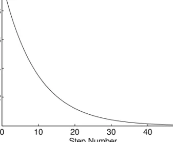
The formula in Step 4 for decreasing s gives an exponential decay of (s−1), as shown in Figure 1. The value of smin should generally be set to
0 10 20 30 40 50 1 1.2 1.4 1.6 1.8 2 Step Number s
Figure 1: The decrease of the value of s in the Fuzzy Steps approach, using γ = 0.9
a value slightly higher than 1, for example, 1.001. The two-mode k-means algorithm is performed at the end of the Fuzzy Steps method, to ensure that a crisp solution is obtained. Although the two-mode k-means algorithm was defined as a crisp algorithm in Section 2.2, it can also be used in combination with fuzzy initial partitions
It is possible that the optimization algorithm gets stuck in a saddle point. This happens if two or more row or column clusters become equal. In that case, these clusters and their corresponding cluster membership values will remain equal for any value ofs. Preliminary tests with the algorithm suggest that it often reaches a saddle point, if the starting value of s is too high. Therefore, it is important not to set the starting value of s too high, for example, s≤1.2.
5
Simulation Study
To compare the performance of the algorithms described in the previous sec-tions, we use a large-scale simulation study. The simulation study aims to determine which of the algorithms perform well under most circumstances and to compare the algorithms thoroughly under varying circumstances. The simulation study also determines how well the algorithms can retrieve a clus-tering structure. First, we describe the setup of the simulation study and how the results are represented. We then give the results of the simulation
study and interpret them.
5.1
Setup of the Simulation Study
Many papers discussing two-mode clustering algorithms often only perform a small simulation study. However, the performance of the optimization methods may depend strongly on the features of the data set. Therefore, we will perform a larger simulation study to compare the methods.
We generate the data matrix X in every problem instance by simulating
P, Q, V, and E, and then using (1) to construct X. Generating simulated data this way comes natural and has the advantage that some clustering structure exists in the data. Also, the P, Q, and V used in generating X
can give a useful upper bound on the optimal value of f(P,Q,V).
A large number of factors can be varied in a simulation study for two-mode clustering, such as the values of n, m, K, and L, the size and the distribution of the errors, the number of elements in the clusters, and the locations of the cluster centers. Using a full factorial design with seven or more factors and multiple levels per factor, would require a prohibitively large number of simulations. Therefore, the number of factors and the number of levels for each factor are limited as follows.
The simulation study is set up using a three-factor design, and is loosely based on the approach of Milligan (1980). The first factor is the size of the data matrix Xand the number of clusters. The three levels of this factor are as follows.
• First level: n= 60, m = 60, and K =L= 6.
• Second level: n= 150, m= 20, and K =L= 5.
• Third level: n=m= 100, and K =L= 3.
The second factor is the size of the error perturbations. All elements of
E are normally distributed with mean 0 and standard deviation equal to 0.5, 1, or 2 for the three levels of this factor. Standard deviations of 0.5 and 1 give a reasonable amount of noise in the simulated data, whereas a standard deviation of 2 can make clustering difficult. The third factor is the distribution of the objects over the clusters. For the first level of this factor all objects are divided over the clusters with equal probability. For the second and third levels, one cluster contains exactly 10% respectively 60% of the objects. The remaining objects are then divided over the remaining clusters with uniform probability. Constructing one cluster with 10% of the objects represents a small deviation from a uniform distribution, whereas a cluster with 60% constitutes a large deviation.
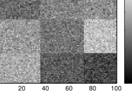
1 20 40 60 80 100 1 20 40 60 80 100 −2 −1 0 1 2
Figure 2: Graphical representation of simulated data set with sizes n =m= 100, K =L= 3, error standard deviation 0.5, and a uniform distribution of the objects over the clusters.
Empty clusters are not allowed in the generated data sets. If a simulated data set contains an empty cluster, it is discarded and another data set is simulated. Finally, the locations of the cluster centersvkl are chosen by
ran-domly assigning the numbers Φ( i
K×L+1), i= 1, . . . , K×L to the elements of
V, where Φ(.) is the inverse standard normal cumulative distribution func-tion. As a result, the elements of V appear standard normally distributed, and a fixed minimum distance between the cluster centers is assured. Note that this setup of the simulation study does not account for certain features of empirical data sets, such as heteroscedasticity and non-normality.
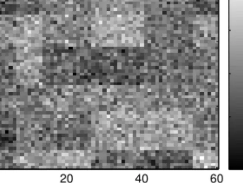
We visualize the effects of some of these choices in Figures 2-4. These figures give a visual representation of the simulated X for various levels of the factors. In these figures, the rows and columns are ordered according to their cluster. The values of the elements of Xare represented by colors, and similar colors correspond to similar numerical values for the elements of X. The color bars at the right-hand side show what values the colors represent. Figure 2 gives an example of a data set, where the choices for the levels of the factors ensure that the original clusters can easily be recognized. In Figure 3, the original clusters are more difficult to recognize, and in Figure 4, this is almost impossible. The optimal clustering should generally be easier to find, when the number of clusters is low, the error standard deviation is small and the objects are evenly divided over the clusters.
These three factors give a total of 3×3×3 = 27 possible combinations. To avoid drawing spurious conclusions based on a single data set, we simulate 50 data sets for each combination and all five methods are performed for each data set. In total, 6750 clustering methods are performed.
1 20 40 60 1 20 40 60 −4 −2 0 2 4
Figure 3: Graphical representation of simulated data set with sizes n =m= 60, K = L = 6, error standard deviation 1 and 10% of the objects in one cluster. 1 20 40 60 1 20 40 60 −6 −4 −2 0 2 4 6
Figure 4: Graphical representation of simulated data set with sizes n =m= 60, K = L = 6, error standard deviation 2 and 60% of the objects in one cluster.
and Qrandom by simply assigning each row and column object to one of the clusters with equal probability. This choice is used for the Multistart AE and Multistart k-means methods. However, many other optimization methods perform better when the initial partitions are relatively good. Therefore, the initial partitions of the Simulated Annealing, Tabu Search, and Fuzzy Steps methods are chosen by applying the two-mode k-means algorithm to a randomly chosen partition.
Some algorithms also require choosing additional parameters. The pa-rameters of these algorithms are chosen as follows:
• Multistart Alternating Exchanges: The Multistart Alternating Ex-changes method performs the Alternating ExEx-changes algorithm 10 times.
• Multistart k-means: The Multistart k-means method performs the k -means algorithm 500 times.
• Simulated Annealing: Initial temperature T=10, r = 2(nL +mK), γ = 0.85, andtmax = 10.
• Tabu Search: The length of the tabu list is 2pn(K−1) +m(L−1) and the number of iterations tmax = 6
p
n(K −1) +m(L−1).
• Multistart Fuzzy Steps: The initial value of s is 1.05, the fuzzy step size γ is 0.9, and the threshold value smin is 1.001. The Fuzzy Steps
algorithm is repeated 10 times for every simulated data set.
The values of these parameters have been chosen after some experimentation, and should give an adequate performance and a comparable computation time for the five methods.
We use multiple criteria to evaluate the results of the simulation study. First, we do not use the value of f(P,Q,V), but the Variance Accounted For (VAF) criterion. The VAF criterion is defined as
VAF = 1− PK k=1 PL l=1 Pn i=1 Pm j=1pikqjl(xij −vkl) 2 Pn i=1 Pm j=1(xij −x)¯ 2 , (11) where ¯x = (N M)−1Pn i=1 Pm
j=1xij. It can be derived that maximizing VAF
corresponds to minimizing f(P,Q,V). The optimal value of VAF ranges from 0 to 1 and is equivalent to the R2-measure used in regression analysis.
We report the average VAF value for all algorithms and the average VAF of the Pand Q used to generate the data.
Second, we report the average Adjusted Rand Index (ARI), which was introduced by Hubert and Arabie (1985). This metric is used to show how well the clustering found by the algorithms approximates the original clus-tering. It is invariant with respect to the ordering of the clusters, which is arbitrary in two-mode clustering. ARI is based on the original Rand Index, which is defined as the fraction of the pairs of elements on which the two clusterings agree. The original Rand index can only take values from 0 to 1. If random partitions are selected, the expected value of the Rand index lies between 0 and 1, and depends on the parameters of clustering problem. To ensure a constant expectation, the ARI is a linear function of the Rand index, so that its expectation is always 0 and its maximum value is 1. It is defined as ARI = PP i=1 PP j=1 aij 2 −PP i=1 ai. 2 PP j=1 a.j 2 / a2 1 2[ PP i=1 ai. 2 +PP j=1 a.j 2 ]−PP i=1 ai. 2 PP j=1 a.j 2 / a2, (12) where aij is the number of elements of X that are simultaneously part of
cluster i of the original clustering and cluster j of the retrieved clustering, ai. = P jaij, a.j = P iaij, and a = P i P
jaij. Here we consider a pair of
elements to be in the same cluster only if they are both part of the same column cluster and of the same row cluster.
The final criterion used to compare the algorithms is the average CPU time required by the algorithms, which is of great practical interest. All algorithms are written in the matrix programming language Matlab 7, and are executed on a Pentium IV 2.8 GHz computer.
Dolan and Mor´e (2002) discuss a convenient tool, calledperformance pro-files, for graphically representing the distribution of the results of a simulation study. Performances profiles are especially useful when trying to determine which algorithms perform reasonably well almost every time the algorithm is run. They can be constructed as follows. First, one has to identify a performance measure. We will use the VAF criterion for this and define VAF(p,s) as the VAF achieved by algorithm s in problem instance p. Then, the performance ratio ρ(p,s) is defined as
ρ(p,s) = maxsVAF
(p,s)
VAF(p,s) . (13)
Finally, the cumulative distribution function of the performance ratio can be computed as
Φ(s)(τ) = 1 50#{ρ
(p,s)≤τ;p= 1, . . . ,50}. (14)
By drawing Φ(s)(τ) in one figure for all algorithms, the performance of the algorithms can be compared quite easily.
Table 1: Average VAF for data sets with n=m= 60, K =L= 6.
object distribution uniform distribution 10%-cluster 60%-cluster error st. dev. .5 1 2 .5 1 2 .5 1 2 Multistart AE .7672 .4604 .1886 .7602 .4608 .1918 .7209 .4167 .1838 Multistartk-means .7693 .4616 .1883 .7667 .4610 .1912 .7379 .4229 .1834 Simulated Annealing .7553 .4554 .1890 .7442 .4498 .1913 .7068 .4110 .1864 Tabu Search .7036 .4360 .1673 .7066 .4356 .1728 .7010 .3968 .1678 Multistart Fuzzy Steps .7637 .4607 .1897 .7617 .4604 .1925 .7247 .4179 .1871
Original partition .7693 .4613 .1799 .7667 .4605 .1810 .7413 .4215 .1568
Table 2: Average VAF for data sets with n= 150, m= 20, K =L= 5.
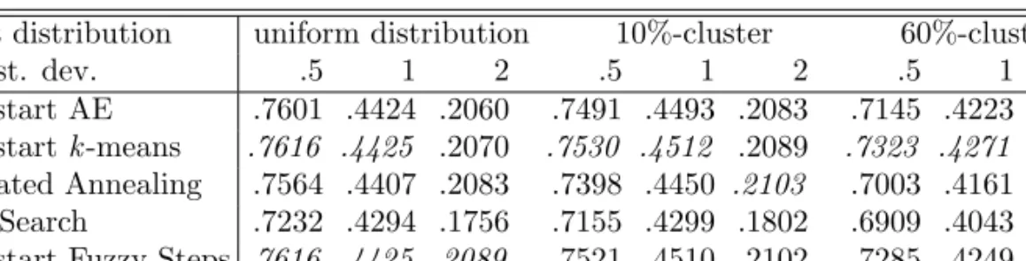
object distribution uniform distribution 10%-cluster 60%-cluster error st. dev. .5 1 2 .5 1 2 .5 1 2 Multistart AE .7601 .4424 .2060 .7491 .4493 .2083 .7145 .4223 .2104 Multistartk-means .7616 .4425 .2070 .7530 .4512 .2089 .7323 .4271 .2121 Simulated Annealing .7564 .4407 .2083 .7398 .4450 .2103 .7003 .4161 .2138
Tabu Search .7232 .4294 .1756 .7155 .4299 .1802 .6909 .4043 .1870 Multistart Fuzzy Steps .7616 .4425 .2089 .7521 .4510 .2102 .7285 .4249 .2131 Original partition .7615 .4378 .1742 .7529 .4458 .1727 .7321 .4157 .1607
5.2
Simulation Results
We will now give the results of the simulation study. Tables 1-3 show the average VAF values of all algorithms for each combination of the factors. The results of the best performing algorithms are shown in italics, for each combination of the factors. The average VAF value of the original partition is also shown.
From these tables, it is clear that the optimization methods with a Multi-start heuristic perform very well, in particular the MultiMulti-startk-means meth-ods. It always has the best average performance when the error standard deviation is 0.5 or 1. The results are somewhat different in data sets with an error standard deviation of 2. The best performance is then often achieved by the Multistart Fuzzy Steps method. The Multistart AE and the Simulated Annealing methods often also have a good performance. The Tabu Search method does not perform as well as the other algorithms in the simulated data sets.
Tables 4-6 give the average values of the Adjusted Rand Index, based on the original P and Q. The best results in these tables are again given
Table 3: Average VAF for data sets withn =m = 100,K =L= 3.
object distribution uniform distribution 10%-cluster 60%-cluster error st. dev. .5 1 2 .5 1 2 .5 1 2 Multistart AE .7032 .3692 .1317 .6884 .3524 .1225 .6749 .3392 .1228 Multistartk-means .7032 .3692 .1317 .6884 .3527 .1226 .6768 .3392 .1233
Simulated Annealing .7032 .3692 .1317 .6840 .3511 .1221 .6663 .3337 .1208 Tabu Search .6772 .3533 .1287 .6656 .3444 .1195 .6530 .3311 .1192 Multistart Fuzzy Steps .7032 .3692 .1317 .6856 .3527 .1218 .6762 .3392 .1219 Original partition .7032 .3690 .1302 .6884 .3525 .1198 .6768 .3392 .1211
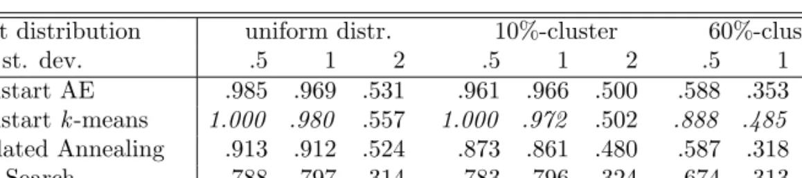
Table 4: Average Adjusted Rand Index in data sets with n = m = 60, K =L= 6.
object distribution uniform distr. 10%-cluster 60%-cluster error st. dev. .5 1 2 .5 1 2 .5 1 2 Multistart AE .985 .969 .531 .961 .966 .500 .588 .353 .124 Multistartk-means 1.000 .980 .557 1.000 .972 .502 .888 .485 .133
Simulated Annealing .913 .912 .524 .873 .861 .480 .587 .318 .130 Tabu Search .788 .797 .314 .783 .796 .324 .674 .313 .106 Multistart Fuzzy Steps .966 .966 .564 .980 .960 .516 .698 .370 .132
in italics. These tables are especially useful for determining the absolute performance of the algorithms. It is clear that a high value of the ARI almost always corresponds to a high value of VAF. In addition, the original partition is often exactly retrieved when the error standard deviation is small and all clusters have approximately the same numbers of objects.
The best performing algorithm usually has an average Adjusted Rand Index above 90% or even 99% if the conditions of the simulated data sets are favorable. This fraction rapidly decreases however, when the problem instances become harder. The original partitions are especially hard to re-trieve, if the error standard deviation is 2 or if 60% of the objects are located in one cluster. The Adjusted Rand Index never becomes negative or very close to 0, which indicates that it always is possible to retrieve some of the structure in the data set.
Another important conclusion is that the differences in the average Ad-justed Rand Indices between the methods can be large. The difference can sometimes be as large as 30%, whereas the differences in VAF are just a few percentage points. Therefore, the choice of the optimization method can be quite important, if one wants to find the ‘true’ clustering.
Table 5: Average Adjusted Rand Index in data sets with n = 150, m= 20, K =L= 5.
object distribution uniform distr. 10%-cluster 60%-cluster error st. dev. .5 1 2 .5 1 2 .5 1 2 Multistart AE .990 .880 .340 .975 .850 .337 .680 .428 .159 Multistartk-means .994 .882 .364 .994 .869 .345 .957 .595 .173
Simulated Annealing .960 .854 .381 .923 .796 .348 .635 .367 .171 Tabu Search .855 .773 .187 .864 .704 .185 .654 .349 .113 Multistart Fuzzy Steps .994 .883 .378 .988 .865 .351 .854 .491 .167
Table 6: Average Adjusted Rand Index in data sets with n = m = 100, K =L= 3.
object distribution uniform distr. 10%-cluster 60%-cluster error st. dev. .5 1 2 .5 1 2 .5 1 2 Multistart AE 1.000 .992 .858 1.000 .978 .749 .984 .990 .749 Multistartk-means 1.000 .992 .858 1.000 .984 .752 1.000 .990 .786
Simulated Annealing 1.000 .992 .859 .976 .962 .721 .937 .931 .641 Tabu Search .878 .884 .802 .911 .898 .642 .906 .915 .611 Multistart Fuzzy Steps 1.000 .992 .860 .977 .984 .721 .992 .990 .704
Table 7: Average CPU time of all algorithms in seconds.
size of data sets n=m= 60 n= 150,m= 20 n=m= 100 error st. dev. .5 1 2 .5 1 2 .5 1 2 Multistart AE 7.5 9.1 13.4 12.0 14.6 17.5 8.3 9.4 14.5
Multistartk-means 12.4 16.1 19.1 12.0 16.6 18.2 8.4 10.3 15.2 Simulated Annealing 22.8 23.0 24.1 28.9 30.9 28.9 27.0 29.8 35.4 Tabu Search 24.8 25.3 25.4 33.2 30.0 29.3 25.0 25.2 25.0 Multistart Fuzzy Steps 7.5 10.5 20.9 7.1 10.9 19.4 4.1 6.8 15.7
Finally, we give the average CPU time in seconds used by all methods in Table 7, for each problem size and value of the error standard deviation. Note that the CPU times strongly depend on the type of computer used and how the methods have been implemented. They should only serve as a general indication of the amount of computation that optimization methods require. The impact of the distribution of the objects over the clusters on the computation time is small and is not shown here. The size of the error stan-dard deviation has a clear positive effect on the computation time, especially for the Multistart Fuzzy Steps method. A higher error standard deviation also leads to longer computation times for the Alternating Exchanges and the two-mode k-means algorithms.
The most important determinants of the CPU times of the methods are the size of the data set and the number of clusters. The computation time does not increase withm,n,K, andLfor all algorithms in the same manner. Therefore, the choice of the method should depend on the size of these factors. The computational load of the Simulated Annealing and Tabu Search meth-ods is somewhat greater than for the other optimization methmeth-ods, though the computation times of the methods are still roughly comparable.
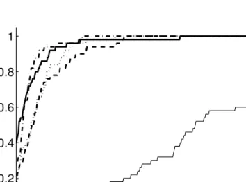
The average VAF values in Tables 1-3 do not show the distribution of the VAF values. For example, it is possible that a method usually performs well, but occasionally gives very poor results. We will show performance profiles of the VAF values for all methods. As drawing these profiles for each of the 27 combinations of the factors requires too much space, we will give three examples. These examples are shown in Figures 5-7.
Figure 5 gives a performance profile of 50 data sets with a low error stan-dard deviation. The value of the graph at the y-axis gives the fraction of times that a method achieved the best VAF value of all method. The Mul-tistart k-means method found the best partition in every problem instance and the Multistart AE method also performed well. Most methods, except Tabu Search, retrieved the initial partition in more than 50% of the problem
1 1.05 1.1 1.15 1.2 0 0.2 0.4 0.6 0.8 1 τ Φ (s) ( τ )
Figure 5: Performance profile of data sets with sizesn=m= 60,K =L= 6, error standard deviation 0.5, and a uniform distribution of the objects. The lines represent the methods Multistart AE (dashed line), Multistartk-means (dotted line), Simulated Annealing (dash-dot line), Tabu Search (thin, solid line), and Multistart Fuzzy Steps (thick, solid line).
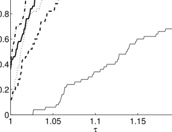
1 1.05 1.1 1.15 1.2 0 0.2 0.4 0.6 0.8 1 τ Φ (s) ( τ )
Figure 6: Performance profile of data sets with sizes n = 150, m = 20, K = L = 5, error standard deviation 2, and one cluster containing 10% of the objects. The lines represent the methods Multistart AE (dashed line), Multistartk-means (dotted line), Simulated Annealing (dash-dot line), Tabu Search (thin, solid line), and Multistart Fuzzy Steps (thick, solid line).
1 1.05 1.1 1.15 1.2 0 0.2 0.4 0.6 0.8 1 τ Φ (s) ( τ )
Figure 7: Performance profile of data sets with sizes n = 150, m = 20, K = L = 5, error standard deviation 2, and one cluster containing 60% of the objects. The lines represent the methods Multistart AE (dashed line), Multistartk-means (dotted line), Simulated Annealing (dash-dot line), Tabu Search (thin, solid line), and Multistart Fuzzy Steps (thick, solid line).
instances.
Figures 6 and 7 show performance profiles of data sets with a large error standard deviation, where the optimal partition was hard to find. In these cases, no algorithm performed at least as good as all others in every problem instance. The Simulated Annealing and Multistart Fuzzy Steps methods of-ten performed well. The performance of the Multistart AE, and Multistart
k-means was somewhat worse. The Tabu Search method is clearly outper-formed by other methods. In both figures, the best average VAF value was achieved by the Simulated Annealing method.
The conclusions of the simulation study can be summarized as follows.
• The Multistart k-means method has the best average performance in most situations with a small amount of error.
• The Multistart Fuzzy Steps method often is the best performing method if the amount of error is high, although its overall performance is slightly worse than that of the Multistart k-means method.
• The Multistart AE and Simulated Annealing methods have a good overall performance, but usually not as good as the Multistartk-means
and Multistart Fuzzy Steps methods. The performance of the Tabu Search method seems to be inferior for the simulated data sets.
• The average Adjusted Rand Index ranges from 14% to 100% in the simulated data sets, and is significantly influenced by the choice of the algorithm and by varying the factors of the simulation study
• Performance profiles show that the performance of each algorithm varies greatly when the algorithm is performed multiple times. There-fore, the Multistart heuristic of algorithms seems to be a very useful strategy.
6
Empirical Data
Here, we present an empirical data set to illustrate two-mode clustering. As marketing is an important area of application for clustering methods, we will use a data set from this area. The data set is used to compare the algorithms and to determine whether the conclusions of the simulation study are valid in a practical data set.
The data set is based on a questionnaire about the Internet. It consists of evaluations of 22 statements about the Internet by 194 respondents. The statements were evaluated using a sevenpoint Likert scale, ranging from 1 -completely disagree to 7 - -completely agree. The average scores in the data set can differ significantly per individual and per statement. A sample run of the two-mode clustering methods shows that, if the raw data set is used, the individuals and the statements will mostly be clustered based on their average scores. We correct for this problem by double centering X, that is, by replacing each xij with ˜xij, where
˜ xij =xij − 1 n n X i0=1 xi0j − 1 m m X j0=1 xij0 + 1 nm n X i0=1 m X j0=1 xi0j0, (15)
so that the column and row averages of X˜ are zero.
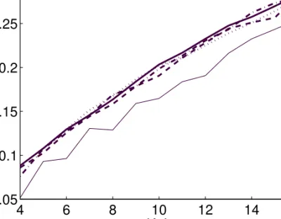
As it is not clear what numbers of clusters should be chosen, we use the following procedure for choosing K and L. First, we perform the clustering methods onX˜, for allK and Lsuch thatK+L=i, fori= 4. . .16. For each valueiwe use the optimization method and values ofK andLthat yield the best VAF. For each value of i and for each method, the best resulting VAF value is shown in Figure 8. The algorithms use the same parameters as in the simulation study.
4 6 8 10 12 14 16 0.05 0.1 0.15 0.2 0.25 0.3 K+L VAF
Figure 8: Best VAF values found in Internet data set, for K+L= 4. . .16. The lines represent the methods Multistart AE (dashed line), Multistart k -means (dotted line), Simulated Annealing (dash-dot line), Tabu Search (thin, solid line), and Multistart Fuzzy Steps (thick, solid line).
The Multistart k-means, Simulated Annealing, and the Multistart Fuzzy Steps methods all had good performances. The Multistart Alternating Ex-changes method performed slightly worse, and the Tabu Search method per-formed rather poorly. These results support the conclusions of the simulation study.
The maximum VAF value shown in Figure 8 increases smoothly with the number of clusters and so it is not entirely clear which values of K and L should be chosen. We decide to use K = L = 5 for further interpretations, which gives a best VAF value of 20.3%. The differences between the clus-ter cenclus-ters are shown in Table 8 in combination with the sizes (number of elements) of the clusters. The differences between the cluster centers are rea-sonably large. One of the statement clusters (columns) consists of a single statement, suggesting that this statement might be an outlier.
The statements in each statement cluster are shown in Table 9. These statement clusters have quite clear interpretations. Whereas the first cluster only consists of one statement, the second cluster mainly consists of state-ments that consider using the Internet expensive. The statestate-ments in the third cluster generally apply to experienced Internet users. The statements in the
Table 8: Average evaluations per cluster, cluster sizes, and interpretations.
respondent statement clusters
clusters 1 2 3 4 5 size interpretation 1 -1.53 0.72 -0.19 -0.34 0.74 34 price-conscious 2 1.69 0.00 -0.32 0.44 -0.60 55 safety-conscious 3 -1.51 -1.25 0.91 -0.19 0.12 26 experts 4 -2.07 0.11 0.36 0.31 -1.05 38 enthusiasts 5 1.88 0.09 -0.33 -0.48 1.09 41 skeptics size 1 4 8 6 3
interpret. regulation expensive experience enthusiastic unreliable
fourth cluster are associated with people who are enthusiastic about the In-ternet. The statements in the fifth cluster consider the Internet unreliable. It is also possible to interpret the respondent clusters, by using the interpreta-tions of the statement clusters and the values of the cluster centers in Table 8. The respondents in the first cluster mainly think that using the Internet is expensive, but they still like it. The second cluster consists of people, who mainly want more regulation on the content of web sites. Parents of young children could be in this cluster. The third cluster of respondents consists of experienced Internet users. Even though they find using the Internet quite cheap, they seem to have lost some of their enthusiasm about it. The fourth cluster is a group of ordinary Internet users, who think positively about the Internet. The respondents in the final cluster seem to dislike using the In-ternet and think it is unreliable. All these interpretations are summarized in Table 8.
The clustered data set is graphically represented in Figure 9, as was done before with simulated data sets in Figures 2-4. The bar at the right-hand side of the figure shows to what values the colors refer. The clusters of the data matrix can easily be recognized, though they can account for only 20.3% of the total variance.
The Internet data set gives a useful example of how two-mode clustering can summarize the information in a data set. The interpretations of both row and column clusters seem quite natural. Two-mode clustering not only divides the respondents and the statements into clusters, but also shows what the opinions of the people in each cluster are.
Table 9: Statement clusters in Internet data set, with interpretations of the clusters between brackets.
Cluster 1 (regulation):
The content of web sites should be regulated
Cluster 2 (expensive):
Internet offers many possibilities for abuse Internet phone costs are high
The costs of surfing are high
The prices of Internet subscriptions are high
Cluster 3 (experience):
Paying using the Internet is safe
I always attempt new things on the Internet first I know much about the Internet
I like surfing
I like to be informed of important new things I often speak with friends about the Internet I regularly visit web sites recommended by others Internet is addictive
Cluster 4 (enthusiastic):
Internet is fast Internet is easy to use
Internet is the future’s means of communication Internet is user-friendly
Internet offers unbounded opportunities Surfing the Internet is easy
Cluster 5 (unreliable):
Internet is unreliable
Transmitting personal data using the Internet is unsafe Internet is slow
Figure 9: Graphical representation of the Internet data set, ordered by clus-ters using K =L= 5.
7
Conclusions
Two-mode clustering seems a powerful statistical technique. However, var-ious algorithms exist but no algorithm is guaranteed to find the optimal clustering. Therefore, it is still unclear which algorithm should be used in practice. We have tried to alleviate these problems, by giving an overview of existing algorithms and introducing several new methods. Five methods have been compared. All methods use one of the heuristics Multistart, Tabu Search, and Simulated Annealing.
A simulation study has been performed to compare these methods and to determine how effective they are at finding the optimal clustering. A full-factorial design was used to assess the effects of characteristics of the clustering problem on the performance of the methods. The sizes of the data matrix, the number of clusters, the size of the errors and the distri-bution of the objects over the clusters were varied in the simulation design. The optimal clustering is often much easier to find if the number of clusters and the size of the errors is small, and if all clusters have approximately the same size. It turns out that the application of the Multistart heuristic in combination with thek-means algorithm usually has the best average perfor-mance, especially if the problem is easy. As it requires relatively little CPU time and is easy to implement without supervision, we recommend using
this algorithm for most instances. When optimal clustering is hard to find, the Simulated Annealing and Multistart Fuzzy Steps methods often perform best. As the optimal clustering is probably hard to find in empirical data sets of reasonably large size, these algorithms can be useful in these cases. Using Multistart in combination with the Alternating Exchanges algorithm often also performs well. The performance of the Tabu Search method generally is inferior; we do not recommend using this algorithm in conditions similar to this simulation study.
The results of the methods on an empirical data set did not deviate from what we found in the simulation study. The empirical data set also gives a useful example of the potential applications of two-mode clustering. The clusters found in this data set are meaningful and provide additional insight. Research in the area of two-mode clustering algorithms is still ongoing and far from complete. For example, we cannot exclude the possibility that some algorithms can be improved by choosing their parameters differently. Besides further theoretical research, further practical experience also is re-quired. Practice can show the real merits and drawbacks of using two-mode clustering.
References
BEZDEK, J. C. (1981), Pattern recognition with fuzzy objective function algorithms, New York: Plenum Press.
BOCK, H. H. (1974), Automatische klassifikation, G¨ottingen: Vandenhoeck & Ruprecht.
CASTILLO, W., and TREJOS, J. (2002), “Two-mode partitioning: Review of methods and application of tabu search,” inClassification, clustering and data analysis, Eds., K. Jajuga, A. Sololowksi, and H. Bock, Berlin: Springer, 43-51.
DESARBO, W. S. (1982), “Gennclus: New models for general nonhierarchi-cal clustering analysis,” Psychometrika, 47(4), 449-475.
DOLAN, E. D., and MOR´E, J. J. (2002), “Benchmarking optimization software with performance profiles,” Mathematical Programming, 91, 201-213.
GAUL, W., and SCHADER, M. (1996), “A new algorithm for two-mode clustering,” in Data analysis and information systems, Eds., H. Bock and W. Polasek, Heidelberg: Springer, 15-23.
GLOVER, F. (1986), “Future paths for integer programming and links to artificial intelligence,” Computers and Operations Research, 13, 533-549.
GROENEN, P. J. F., and JAJUGA, K. (2001), “Fuzzy clustering with squared Minkowski distances,” Fuzzy Sets and Systems, 120, 227-237. HANSOHM, J. (2001), “Two-mode clustering with genetic algorithms,” in
Classification, automation, and new media, Berlin: Springer, 87-93. HARTIGAN, J. A. (1975), Clustering algorithms, New York: John Wiley
and Sons.
HEISER, W. J., and GROENEN, J. (1997), “Cluster differences scaling with a within-clusters loss component and a fuzzy succesive approximation strategy to avoid local minima,” Psychometrika, 62(1), 63-83.
HUBERT, L., and ARABIE, P. (1985), “Comparing partitions,” Journal of Classification, 2, 193-218.
VAN LAARHOVEN, P. J. M., and AARTS, E. H. L. (1987), Simulated annealing: Theory and applications, Eindhoven: Kluwer Academic Publishers.
MILLIGAN, G. W. (1980), “An examination of the effect of six types of error perturbation on fifteen clustering algorithms,” Psychometrika,
45(3), 325-342.
NOMA, E., and SMITH, D. R. (1985), “Benchmark for the blocking of sociometric data,” Psychological Bulletin, 97(3), 583-591.
TREJOS, J., and CASTILLO, W. (2000), “Simulated annealing optimiza-tion for two-mode partioptimiza-tioning,” in Classification and information at the turn of the millenium, Eds., W. Gaul and R. Decker, Heidelberg: Springer, 135-142.
TSAO, E. C. K., BEZDEK, J. C., and PAL, N. R. (1994), “Fuzzy Kohonen clustering networks,” Pattern recognition, 27(5), 757-764.
VAN MECHELEN, I., BOCK, H. H., and DE BOECK, P. (2004), “Two-mode clustering methods: A structured overview,” Statistical Methods in Medical Research,13, 363-394.