DEVELOPMENT OF PTO-SIM: A POWER PERFORMANCE MODULE FOR THE
OPEN-SOURCE WAVE ENERGY CONVERTER CODE WEC-SIM
Ratanak So Asher Simmons
Ted Brekken
School of Electrical Engineering and Computer Science Oregon State University
Corvallis, Oregon USA
Kelley Ruehl∗ Carlos Michelen Water Power Department Sandia National Laboratories
Albuquerque, NM USA Email: [email protected]
ABSTRACT
WEC-Sim (Wave Energy Converter-SIMulator) is an open-source wave energy converter (WEC) code capable of simulat-ing WECs of arbitrary device geometry subject to operational waves. The code is developed in MATLAB/Simulink using the multi-body dynamics solver SimMechanics, and relies on Bound-ary Element Method (BEM) codes to obtain hydrodynamic coef-ficients such as added mass, radiation damping, and wave exci-tation. WEC-Sim Version 1.0, released in Summer 2014, mod-els WECs as a combination of rigid bodies, joints, linear power take-offs (PTOs), and mooring systems. This paper outlines the development of PTO-Sim (Power Take Off-SIMulator), the WEC-Sim module responsible for accurately modeling a WEC’s con-version of mechanical power to electrical power through its PTO system. PTO-Sim consists of a Simulink library of PTO compo-nent blocks that can be linked together to model different PTO systems. Two different applications of PTO-Sim will be given in this paper: a hydraulic power take-off system model, and a direct drive power take-off system model.
INTRODUCTION
Sandia National Laboratories (SNL) and the National Re-newable Energy Laboratory (NREL) have jointly developed WEC-Sim (Wave Energy Converter-SIMulator), an open-source
∗
wave energy converter (WEC) design tool capable of running on a standard personal computer. WEC-Sim simulates WECs of ar-bitrary device geometry subject to operational waves [1]. The code is developed in MATLAB/Simulink using the multi-body dynamics solver SimMechanics, and relies on Boundary Ele-ment Method (BEM) codes to obtain hydrodynamic coefficients such as added mass, radiation damping, and wave excitation. The WEC-Sim hydrodynamic solution has been verified through code-to-code comparison, and has undergone preliminary vali-dation through comparison to experimental data [2] [3] [4] [5]. Further validation of the WEC-Sim code will be performed upon completion of the WEC-Sim validation tank testing, planned for Summer 2015.
Version 1.0 of WEC-Sim, released in Summer 2014, models WECs as a combination of rigid bodies, joints, linear power take-offs (PTOs), and mooring systems. While the Version 1.0 release of the WEC-Sim code was limited to modeling PTOs as sim-ple linear dampers, collaboration with the Energy Systems group at Oregon State University (OSU) has resulted in the develop-ment of PTO-Sim (Power Take Off-SIMulator). PTO-Sim is the WEC-Sim module responsible for accurately modeling a WEC’s conversion of mechanical power to electrical power through its PTO system (or power conversion chain, PCC). It consists of a library of PTO component blocks that can be linked together to model different PTO systems. Each of these PTO library blocks is a model of common PTO components, such as electric gener-Proceedings of the ASME 2015 34th International Conference on Ocean, Offshore and Arctic Engineering
OMAE2015 May 31-June 5, 2015, St. John's, Newfoundland, Canada
OMAE2015-42074
ators, pistons, and accumulators. Two different applications of PTO-Sim will be given in this paper: a hydraulic power take-off system model, and a linear direct drive power take-off system model.
POWER CONVERSION CHAINS
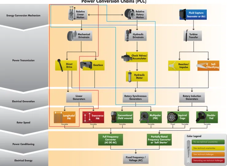
A WEC’s power conversion chain converts the mechanical motion of the WEC into electrical power [6]. The majority of WECs convert the energy from the wave into either relative lin-ear motion, relative rotary motion, or fluid capture. This me-chanical power is then converted into electrical power through the WEC’s PCC. There are many different possible PCC config-urations, as shown in Fig 1. On the left side of the figure is the energy conversion mechanism, and on the right side are differ-ent PCC compondiffer-ents with black arrows indicate possible PCC paths. The Color Legend refers to technological readiness level of each PCC component [7] [8]. This technological readiness level is based on the work in the DNV Recommended Practices which takes into consideration both the degree of the novelty of the technology and its intended application [9].
Based on a survey of the EERE WEC database, there are 34 WEC PCCs that are at a technology readiness level (TRL) 5 or greater [10]. Of these 34 WEC PCCs, 16 use a hydraulic PTO, 11 use a mechanical PTO, and 7 use a turbine, see Fig. 2. Of the 11 mechanical PTOs, 6 are direct drive systems. The results of this survey, and current trends in the WEC industry, drove the devel-opment of hydraulic and direct drive application cases PTO-Sim. These two application cases will be released with future versions of the WEC-Sim code. Since WEC-Sim is an open source code, and there are many different possible PCC configurations, users can create PCC specific models to meet their needs. These can be built based on existing PTO-Sim library blocks, or by creating new PCC component blocks.
PTO-SIM
WEC-Sim consists of a library of different WEC compo-nents, namely: bodies, joints and constraints. These WEC-Sim library blocks can be linked together to model the hydrodynamic behavior of different WEC devices. An example of applying the WEC-Sim code that used PTO-Sim to model the Reference Model 3 (RM3) point absorber is shown Fig. 3. The RM3 was de-signed as part of the DOE-funded Reference Model Project [11]. RM3 is a simple two-body heaving point absorber, consisting of a float and a damping plate. The float is connected to the damp-ing plate through a translational joint which is actuated by the ex-ternal PTO-Sim subsystem that simulates the PTO system. The damping plate is then connected to the seabed through a heave joint that constrains motion relative to the sea floor. This paper specifically focuses on what is inside the PTO-Sim block on the left side of Fig. 3.
PTO-Sim is developed in a similar manner to WEC-Sim, as a library of different PCC components. The PTO-Sim library has been developed based on the possible PCC configurations out-lined in Fig 1. In the following sections, the PTO-Sim compo-nent library will be used to model a hydraulic PTO, and a direct drive PTO. WEC PCCs are complex and device specific, mean-ing that while some PTO models can be built directly from the PTO-Sim library, others will require custom PCC library compo-nents. For the purpose of describing the coupling between PTO-Sim and WEC-PTO-Sim, refer to Fig. 3, where the WEC-PTO-Sim rela-tive displacement and velocity outputs (zRel and zDotRel respec-tively) are the PTO-Sim inputs. Similarly the PTO force (Fpto) is the WEC-Sim input, and the PTO-Sim output for both PTO architectures demonstrated in this paper. These signals are what couple WEC-Sim and PTO-Sim together. In order to demon-strate the functionality of PTO-Sim, the results presented in the following sections use a relative velocity (zDotRel) from WEC-Sim to run the PTO-WEC-Sim simulations, but the PTO-WEC-Sim force (Fpto) was not fed back into the WEC-Sim code (one-way cou-pling). A fully two-way coupling of PTO-Sim with WEC-Sim is under development.
Hydraulic PTO
An example of a hydraulic PTO used in a point absorber is shown in Fig. 4. The piston position and velocity are the rel-ative displacement and velocity between the float and the spar. The first PTO system element is a double acting hydraulic pis-ton pump, “P”. This component directly converts the heave mo-tion of the buoy into a pressurized, bi-direcmo-tional fluid flow. The piston chamber is connected to a rectifying valve via terminals “A” and “B”. This changes the bi-directional flow into a uni-directional flow and passes the fluid on to the rest of the system. The valves “1” through “4” indicate the different flow paths that perform this conversion. Valve “1” delivers fluid to the high pres-sure side of the system where it is stored in the high prespres-sure ac-cumulator “C”. A variable displacement motor, “M”, translates the hydraulic fluid power into rotational energy. The axle of the motor is connected directly (no gearboxes) to a generator axle (“G”) , causing it to spin and generate electricity. The hydraulic motor was chosen to meet the torque and speed requirements. The hydraulic fluid then enters the low pressure side where ac-cumulator “D” provides pressure control. The piston draws fluid from “D”, completing the circuit [12].
The hydraulic PTO model begins with the continuity equa-tion for a compressible fluid, which is used to describe the pres-sures in the piston chamber [13]:
˙
pA=
βe
FIGURE 1. Power conversion chain from mechanical energy to electrical connection to grid. Lower TRLs are novel concepts and higher TRLs are more proven technology. The direct drive PTO path is shown in the red box outline and the hydraulic PTO path is shown in the blue box outline.
˙
pB=
βe Vo+Apz
(−Apz˙−V˙2+V˙3) (2)
The effective bulk modulus of the hydraulic fluid isβe,Vo
is the volume of the piston, andApis the piston area. The
volu-metric flow through valves 1-4 are represented by ˙V1through ˙V4.
The piston and buoy are rigidly connected, and their movement with respect to the spar is the input to the PTO system. The rel-ative motion between the buoy and the spar is represented by the velocity, ˙z(from WEC-Sim).
The four valves in the rectifying circuit are each modeled using the orifice equation:
˙
Vi=CdAv
s 2
ρ(pj−pk)tanh(k1(pj−pk)) (3)
The subscript “i” refers to the valve number.Cdis the
dis-charge coefficient and Av is the cross-section area of the ori-fice. Finally, pj and pk are the pressures on either side of the
valve. The tanhfunction, being differentiable, enables certain control/optimization strategies as well as simplifying the calcu-lations. Also, thetanhfunction multiplied by the pressure dif-ference provides an analytic approximation to the absolute value function, wherek1>>0. The valve area is modeled as a variable
area poppet valve, with the equation:
Av=Amin+ Amax−Amin 2 + Amax−Amin 2 (tanh(k2(pj−pk− pmax+pmin 2 ))) (4) whereAmaxandAminare the maximum and minimum valve areas.
FIGURE 2. Breakdown of PCC types currently used by companies with TRL equal to or greater than 5.
FIGURE 3. RM3 model with PTO-Sim (left) with the animation
(right) [1].
The valve begins to open whenpminis reached. The maximum
pressure,pmaxis the pressure for which the valve is fully opened.
Thetanhfunction in this equation provides a smooth approxi-mation to the step operation of the valve. This is accomplished by choosingk2such that when the pressure difference (pj- pk)
is equal to pmax, the valve area difference (Av-Amin) is equal to Amin. The behavior of the valve is shown in Fig. 5.
The flow into the accumulators “C” and “D” are, respec-tively:
˙
VC=−αDω+V˙1+V˙2 (5)
FIGURE 4. Schematic of the PTO-Sim hydraulic model. The arrow
indicate the direction of flow.
FIGURE 5. Valve opening behavior as a function of pressure
differ-ence across the valve.
˙
VD=αDω−V˙3−V˙4 (6)
whereαis the swashplate angle ratio, which is the instantaneous motor displacement divided by the the maximum motor displace-ment. It is used as a control for the volumetric flow across the motor. Dis the nominal motor displacement, and ω is the ro-tational speed of the generator. For this hydraulic system the swashplate angle ratio is fixed for the simulated sea state.
The pressure in each accumulator is dependent on the in-stantaneous volume of hydraulic fluid in the accumulator:
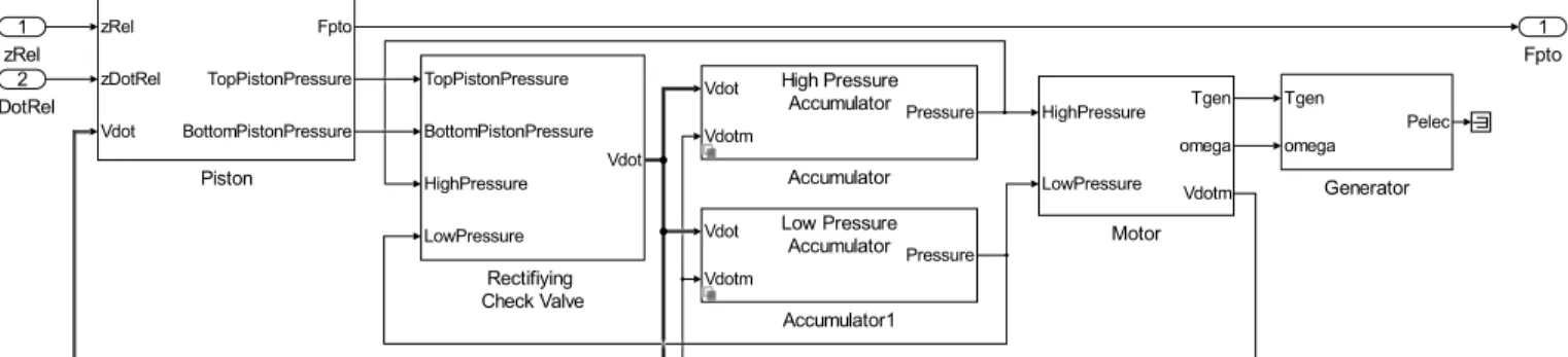
1 Fpto 1 zRel HighPressure LowPressure Tgen omega Vdotm Motor Vdot Vdotm Pressure High Pressure Accumulator Accumulator Vdot Vdotm Pressure Low Pressure Accumulator Accumulator1 TopPistonPressure BottomPistonPressure HighPressure LowPressure Vdot Rectifiying Check Valve Tgen omega Pelec Generator zRel zDotRel Vdot Fpto TopPistonPressure BottomPistonPressure Piston 2 zDotRel
FIGURE 6. Simulink model of the hydraulic system.
pi= pi0 (1−Vi Vi0)
1.4 (7)
wherepi0is the precharge pressure andVi0is the total volume of
the accumulator.
Because the motor axle and generator axle are rigidly con-nected, they have the same torque and opposite rotational direc-tion. This condition leads to the state equation:
˙ ω= 1
Jt
(αD(pC−pD)−bgω−bfω) (8)
The generator torque is represented by bgω, the frictional damping isbfω, andJtis the total mass moment of inertia of the
motor/generator drive train. The frictional damping was chosen to give the generator a 95% efficiency at a speed of 2400 rpm.
Finally, the PTO force is described by the A-B pressure dif-ferential and the piston area under pressure,Ap:
Fpto= (pA−pB)Ap (9)
These equations are contained in PTO-Sim library blocks, representing physical components of the hydraulic PTO system. The complete hydraulic PTO model as implemented using PTO-Sim is shown in Fig. 6.
Simulations. Figures 7 and 8 show a sample (from 200-300 seconds) of the simulation. Figure 7 shows the system in-puts, zRel (relative heave displacement) and zDotRel (relative heave velocity). Figure 8 shows the power produced by the PTO. The blue line,Pabsis the power absorbed at the piston.Pmech, the
power at the axle connecting the motor and generator, is shown
in green. Finally,Pelecis the electrical power at the output of the
generator, is shown in red. The generator model is based on the characteristics of a typical large industrial induction generator. The speed, torque, and efficiency of this motor are taken from a lookup table and used as a simple rotational inertial model.
Electrical power is smaller than mechanical power because the generator block is modeled such that the efficiency of output electrical power is determined by the rotational speed and torque of the generator. In other words, there are some losses in the generator.
The lull in “zDotRel” between simulation time 270 and 280 represents a fairly regular occurrence in typical seas. The near-zero velocity causespjandpkto fall belowpminand the
rectify-ing valve shuts. The system response in this condition is shown in Figs. 9 and 10. Because the fluid is modeled as compressible and the closed valves have abruptly stopped the fluid flow, the fluid in the piston oscillates. This spring-like effect continues until the pressure exceedspmin[14].
DIRECT DRIVE PTO
Alternative to hydraulics, the direct drive power take off has less moving parts which allows a generator to capture power di-rectly from the WEC movement. In this architecture, the PTO uses the relative heave velocity to drive the generator. The stator portion of the generator is contained in the WEC spar, while the buoy contains the magnets. This concept is illustrated in Fig. 11, and modeled using PTO-Sim in Fig. 12. The relative heave ve-locity causes the magnetic field surrounding the coils to change, the fundamental method for generating electricity. While this architecture has fewer power transformation stages and moving parts, it also has no inherent power storage capability (unlike the hydraulic system).
The direct drive approach can be constructed to deliver sin-gle or multiple-phase power by the arrangement of the genera-tor magnets and coils. A three-phase winding was used in this model, enabling a valid comparison with the hydraulic model.
be-200 220 240 260 280 300 −2 −1.5 −1 −0.5 0 0.5 1 1.5 2 Time (s) Velocity (m/s) Piston Velocity
FIGURE 7. Piston velocity for a wave of 3 meters with a dominant
period of 11 seconds. 200 220 240 260 280 300 −0.1 0 0.1 0.2 0.3 0.4 0.5 0.6 0.7 0.8 0.9 Time (s) Normalized Power
Normalized Absorbed, Mechanical, and Electrical Power Pnorm abs Pnorm mech Pnorm elec
FIGURE 8. Absorbed, mechanical, and electrical power.
low.
Tem=k(λsdisq−λsqisd) (10)
wherek=P/2 for rotational generator andk=π/τpmfor a
lin-ear generator. P is the number of poles (Pis greater or equal to 2, even number). τpmis the magnet pole pitch (the distance
200 220 240 260 280 300 −0.5 −0.4 −0.3 −0.2 −0.1 0 0.1 0.2 0.3 0.4 0.5 Time (s) Force (MN) PTO Force
FIGURE 9. PTO force generated by the hydraulic PTO.
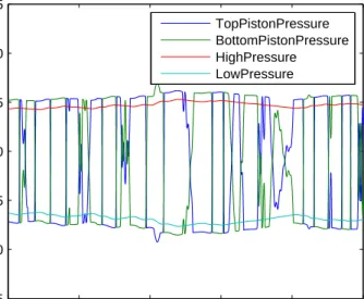
200 220 240 260 280 300 5 10 15 20 25 30 35 Time (s) Pressure (MPa)
Piston Pump and Accumulators Pressures TopPistonPressure BottomPistonPressure HighPressure LowPressure
FIGURE 10. Piston pump and accumulators pressures. A check valve
is open when either the top or bottom piston pressure is greater than the high pressure accumulator or less than the low pressure accumulator.
measured of the magnet from the center of one pole to the center of the next pole). The generator is modeled in the synchronous reference frame, whereλsdis the stator d-axis flux linkage,isqis
the stator q-axis current,λsqis the stator q-axis flux linkage, and isdis the stator d-axis current. Derivation can be found in [15].
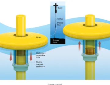
FIGURE 11. Direct Drive: OSU L10. This figure shows the sta-tionary generator coils located inside the spar and the sliding magnet assembly coupled to the float. (Image courtesy of Smithsonian Maga-zine) [16].
FIGURE 12. Schematic of the PTO-Sim direct drive model.
λsq=0, Eq.(10) leads to Eq.(11), which describes the PTO force
for a linear electric machine.
Fpto= (π/τpm)λf disq (11)
The direct drive PTO model presented in this paper is based on [17]. The generator stator consists of three-phase armature windings in 4 slots per phase for a total of 12 slots. There are al-ways 2 pole pairs in the active region at any given time as shown in Fig. 13.
The equivalent electrical circuit (Fig. 14) shows the relation-ship between induced voltagesEa,Eb,andEcand the external
loadsRLoad.RsandLsare the winding resistance and inductance
of the coil.
FIGURE 13. Cross section view of slots and magnets.
Simulations. The PTO was developed and verified with the use of regular waves. Once verified, irregular waves are ap-plied, and the analysis can be focused on understanding the elec-trical power generated by the system. The same “zDotRel” is used as an input for the direct drive PTO model as was used for the hydraulic PTO, see Fig. 7.
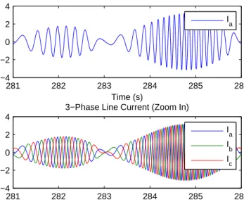
The PTO force, derived in (11), directly follows the relative velocity because of the nature of the direct drive design (no en-ergy storage). Figures 16 and 17 show voltage and current in the external load. It should be noted that the magnitude of the voltage and current depends on the wave climate, and the WEC design parameters [17]. The absorbed and electric power are shown in Fig. 18.
Ec Rs RLoad Ls Rs Ls Rs Ls
FIGURE 14. Back EMF circuit.
200 220 240 260 280 300 −1.5 −1 −0.5 0 0.5 1 1.5 2 Time (s) Force (kN) PTO Force
FIGURE 15. Direct drive PTO force.
Generated Power Comparisons
The usefulness of the PTO-Sim tool is exemplified by com-paring the results from the two different architectures. The out-put electrical power for each PTO architecture is normalized and plotted in Fig. 19. This figure clearly shows the native storage ca-pability of the hydraulic system, which manifests as a smoother power profile. In contrast, the direct drive architecture power output is a direct reflection of the incident sea state.
Although Fig. 19 shows a comparison between the two PTOs, it is hard to determine which PTO system yields more power because in order to do so, the direct drive system would need to have a storage. The purpose of this comparison is to show that each PTO has its pros and cons.
Current WEC-Sim allows the user to get an idea of what
281 282 283 284 285 286 −400 −200 0 200 400 Time (s) Voltage (V)
A Phase Line to Neutral Load Voltage V a 281 282 283 284 285 286 −400 −200 0 200 400 Time (s) Voltage (V)
3−Phase Line to Neutral Load Voltage (Zoom In) V a V b V c
FIGURE 16. Direct drive 3-phase line to neutral load voltage. As
the PTO speed increases, both voltage magnitude and electric frequency increase. 281 282 283 284 285 286 −4 −2 0 2 4 Time (s) Current (A)
A Phase Line Current
I a 281 282 283 284 285 286 −4 −2 0 2 4 Time (sec) Current (A)
3−Phase Line Current (Zoom In)
I a I b I c
FIGURE 17. Direct drive 3-phase current.
the power production will be; with little knowledge of drive-trains/power electronics, etc. However, if the user wants to de-sign a PCC and compare the benefits of different PCC options, that is where PTO-Sim will come to play. It should be noted that, this obviously requires the user to be more knowledgeable and careful when designing the PTO model. Therefore, the goal of designing PTO-Sim is to abstract the end-user from the details
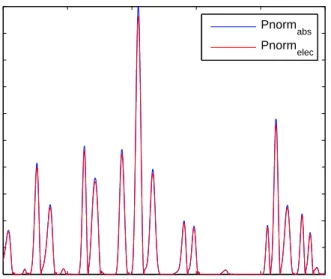
200 220 240 260 280 300 0 0.1 0.2 0.3 0.4 0.5 0.6 0.7 0.8 0.9 1 Time (s) Normalized Power
Normalized Absorbed and Electrical Power Pnorm
abs
Pnorm
elec
FIGURE 18. Absorbed and Electrical Power. Efficiency is calculated
to be about 96 %. 200 220 240 260 280 300 0 0.1 0.2 0.3 0.4 0.5 0.6 0.7 0.8 0.9 1 Time (s) Normalized Power
Normalized Hydraulic and Direct Drive Electrical Power PnormHYD
elec
PnormDD
elec
FIGURE 19. Comparison Between Normalized Hydraulic and Direct
Drive Electrical Power.
but to make the wave energy converter more accessible.
CONCLUSION
This paper illustrates the development and application of PTO-Sim, the WEC-Sim module responsible for accurately
mod-eling the WEC’s conversion of mechanical power to electri-cal power through its PTO system (or power conversion chain, PCC). While the initial release of WEC-Sim, Version 1.0, in-cluded the ability to model a WEC’s PTO system as a simple linear damper, PTO-Sim allows users to model more compli-cated WEC PCCs. To show the functionality of PTO-Sim, two applications of PTO-Sim were given in the paper. One of a hy-draulic PTO system, and one of a direct drive PTO system. These two configurations were chosen because they reflect the two most common WEC PTO systems for WECs with TRL 5+. The sim-ulation results included illustrate the typical high-efficiencies of direct drive systems, but also illustrate the power smoothing (i.e., energy storage) inherent to hydraulic systems.
The current release of the WEC-Sim code, v1.0, includes linear damping to model WEC PTOs. Future work on PTO-Sim includes development of fully two-way coupled WEC-Sim and PTO-Sim models for both the hydraulic and direct drive PTOs. The hydraulic and direct drive PTO-Sim libraries will be in-cluded in future releases of the WEC-Sim code. Also inin-cluded in the future WEC-Sim releases will be example applications of the PTO-Sim library to model hydraulic and direct drive PTO systems based on the work presented in this paper.
ACKNOWLEDGMENT
This research was made possible by support from the Wind and Water Power Technologies Office within the DOE Office of Energy Efficiency & Renewable Energy. The work was sup-ported by Sandia National Laboratories and by the National Re-newable Energy Laboratory. Sandia National Laboratories is a multi-program laboratory managed and operated by Sandia poration, a wholly owned subsidiary of Lockheed Martin Cor-poration, for the U.S. Department of Energys National Nuclear Security Administration under contract DE-AC04-94AL85000. Special thanks to Sam Kanner (University of California Berke-ley) and Sean Casey (Energy Storage Systems, Inc.) for their input on the development of PTO-Sim.
REFERENCES
[1] WEC-Sim. Version 1.0, http://en.openei.org/wiki/WEC-Sim, [Accessed June 2014].
[2] Y. Yu, Ye Li, Kathleen Hallett, and Chad Hotimsky, “De-sign and analysis for a floating oscillating surge wave en-ergy converter,” inProceedings of OMAE 2014, (San Fran-cisco, CA), 2014.
[3] MJ Lawson, Y. Yu, Adam Nelessen, Kelley Ruehl, and Car-los Michelen, “Implementing nonlinear buoyancy and exci-tation forces in the WEC-sim wave energy converter mod-eling tool,” inProceedings of OMAE 2014, (San Francisco, CA), 2014.
[4] Kelley Ruehl, Carlos Michelen, Samuel Kanner, Michael Lawson, and Y. Yu, “Preliminary verification and validation of WEC-sim, an open-source wave energy converter design tool,” inProceedings of OMAE 2014, (San Francisco, CA), 2014.
[5] Y. Yu, Michael Lawson, Kelley Ruehl, and Carlos Miche-len, “Development and demonstration of the WEC-sim wave energy converter simulation tool,” inProceedings of the 2nd Marine Energy Technology Symposium, (Seattle, WA, USA), 2014.
[6] Y. Kamizuru,Development of Hydrostatic Drive Trains for Wave Energy Converters. PhD thesis, RWTH Aachen Uni-versity, Germany, 2014.
[7] M. Reed, R. Bagbey, A. Moreno, T. Ramsey, and J. Rieks, “Accelerating the us marine and hydrokinetic technology development through the application of technology readi-ness levels (TRLs),”Energy Ocean, 2010.
[8] K. Ruehl and D. Bull, “Wave energy development roadmap: design to commercialization,” inOceans, IEEE, 2012. [9] D. N. Veritas, “Recommended practice dnv-rp-a203–
qualification procedures for new technology,” 2001. [10] WHTP marine hydrokinetic technologies database: Project
profile, http://www1.eere.energy.gov/water/hydrokinetic [Accessed Dec. 2014].
[11] Sandia national laboratories: Reference model project (rmp), http://energy.sandia.gov/energy/renewable-energy/water-power/reference-model-project-rmp/ [Ac-cessed Dec. 2014].
[12] S. Casey, “Modeling, simulation, and analysis of two hy-draulic power take-off systems for wave energy conver-sion,” Master’s thesis, Oregon State University, Corvallis, OR, 2013.
[13] H. E. Merritt,Hydraulic control systems. John Wiley, 1967. [14] J. Falnes,Ocean waves and oscillating systems. Cambridge
University Press, 2005.
[15] N. Mohan, “Advanced electric drives,”Minneapolis: MN-PERE, 2001.
[16] E. Rusch, “Catching a wave, powering an electrical grid?,”
Smithsonian Magazine, July 2009.
[17] J. Prudell, M. Stoddard, T. Brekken, and A. von Jouanne, “A novel permanent magnet tubular linear generator for ocean wave energy,” inEnergy Conversion Congress and Exposition, 2009. ECCE 2009. IEEE, pp. 3641–3646, IEEE, 2009.