ISSN 1936-5098
CAE Working Paper #08-02
Default Estimation, Correlated Defaults, and Expert Information by Nicholas M. Kiefer May 2008
Default Estimation, Correlated Defaults, and
Expert Information
Nicholas M. Kiefer
1Cornell University
April 21, 2008
1Cornell University, Departments of Economics and Statistical Science, 490 Uris Hall,
Ithaca, NY 14853-7601, US. email:[email protected]; US Department of the Treasury, Office of the Comptroller of the Currency, Risk Analysis Division, and CRE-ATES, funded by the Danish Science Foundation, University of Aarhus, Denmark. Dis-claimer: The statements made and views expressed herein are solely those of the author, and do not necessarily represent official policies, statements or views of the Office of the Comptroller of the Currency or its staff.
Abstract
Capital allocation decisions are made on the basis of an assessment of creditwor-thiness. Default is a rare event for most segments of a bank’s portfolio and data information can be minimal. Inference about default rates is essential for efficient capital allocation, for risk management and for compliance with the requirements of the Basel II rules on capital standards for banks. Expert information is crucial in inference about defaults. A Bayesian approach is proposed and illustrated using prior distributions assessed from industry experts. A maximum entropy approach is used to represent expert information. The binomial model, most common in appli-cations, is extended to allow correlated defaults yet remain consistent with Basel II. The application shows that probabilistic information can be elicited from experts and econometric methods can be useful even when data information is sparse.
Keywords: Bayesian inference, Basel II, risk management, prior elicitation, small probability estimation
1
Introduction
The efficiency of resource allocation in a modern economy depends crucially on the quality of numerous decentralized decisions on credit allocation. These decisions de-pend on inference about small probabilities, where data information can be sparse but expert information is clearly available. Large, internationally active banks must follow internationally negotiated guidelines. The Basel II (B2) framework (Basel Committee on Banking Supervision (2006)) for calculating minimum capital re-quirements provides for banks to use models to assess credit (and other) risks. All aspects of these models – specification, estimation, validation – will have to meet the scrutiny of national supervisors. These models should be the same ones that sophisticated institutions use to manage their loan portfolios. Banks using internal ratings-based (IRB) methods to calculate credit risks must calculate default prob-abilities (PD), loss given default (LGD), exposure at default (EAD) and effective maturity (M) for groups of homogeneous assets. It can be argued that of these PD is the most important. For very safe assets or for newly-developed assets calculations based on historical data and the frequency estimator may be problematic since few defaults are observed. Estimation of small probabilities has attracted considerable recent attention; see Basel Committee on Banking Supervision (2005), BBA, LIBA, and ISDA (2005), Kiefer (forthcoming) and Pluto and Tasche (2005). Midportfolio asset groups, for which default is still a rare event, typically have some default ex-perience and larger sample sizes. These groups can support models allowing simple forms of default dependence. Expert information remains important.
I focus here on incorporating expert information in estimating the default proba-bilityθ for well-defined portfolio segments. Uncertainty about the default probabil-ity should be modeled the same way as uncertainty about defaults – represented in a probability distribution. A future default either occurs or doesn’t (given the defi-nition). Since we do not know in advance whether default occurs or not, we model this uncertain event with a probability distribution. This model reflects partial knowledge of the default mechanism. Similarly, the default probability is unknown. But there is some information available aboutθin addition to the data information. The simple fact that loans are made shows that some risk assessment is occurring. This information should be organized and incorporated in the analysis in a sensible way, specifically represented in a probability distribution. It can be shown that beliefs that satisfy certain consistency requirements, for example that the believer
is unwilling to make sure-loss bets, lead to measures of uncertainty that combine according to the laws of probability: convexity, additivity and multiplication. See for example DeGroot (1970). This information should be combined with data in-formation as represented in the relevant likelihood function. This combination of information is easy to do once the information is represented in probability distri-butions. The final distribution should represent both data and expert information about the default probability.
Much effort in theoretical econometrics is currently devoted to methods for ex-tracting data information with minimal assumptions. This approach is appealing when there is a great deal of informative data, as illustrated by the fact that most results available and sought are asymptotic. However there is a large class of im-portant practical problems for which there are some, but not much data and there are also experts whose experience and knowledge is relevant. Despite the lack of conclusive data evidence, decisions must be made. In many applied settings profes-sional judgment is expected and discussed at the same level as the statistical model (which is a result of judgment) or the relevance of the data (more judgment). For example judges have guidelines on how to determine whether someone should be admitted as an expert and how much weight to give to the expert’s information. This inference situation is difficult for economists due perhaps to the ambiguity surrounding the way in which expert and data information are combined. Much of this uncomfortable ambiguity can be eliminated by adopting a formal Bayesian approach. Once expert information is cast in terms of probabilities, then analysis proceeds simply by applying the rules of probability. In this approach the econome-trician is faced with two modeling tasks. The first is the familiar task of specifying the likelihood function. The second is specifying the expert information, usually consisting of a limited number of assessments, in terms of a statistical distribution. This paper illustrates the use of informative priors in an important applied set-ting. Explicit use of informative priors is rarely seen in economic applications, though prior or expert information is crucial in any modeling application, including nonparametric applications - see the vivid examples in Dufour, Jouneau-Sion, and Torrs (2007). The quest for objectivity has eliminated the language of prior infor-mation, but simply consider that likelihood functions are not handed to us. At an even more basic level, consider the choice of the covariate list. Bayesian applica-tions in economics are often conducted using objective priors, which yield some of the advantages of the Bayesian approach, most specifically a type of logical
consis-tency and access to powerful computational techniques such as MCMC (see Robert and Casella (2004) and Geweke (2005)) for inference. However the real power of the Bayesian approach is the ability to combine information from all sources coherently. This is especially important when no single source of information dominates. For example, if the data information is overwhelming, there is little gain from precise assessment of a prior; similarly, if there are no data, prior elicitation (perhaps under another name) becomes crucial.
The difficulty in applying the Bayesian approach is that unfamiliar thinking is required. It is not easy to quantify the information or, alternatively, the uncer-tainty about θ. Quantification of uncertainty requires comparison with a standard. One standard for measuring uncertainty is a simple conceptual experiment, such as drawing balls from an urn at random as above, or sequences of coin flips. We might begin by defining events for consideration. Examples of events areA = ”θ ≤0.005”; ”B = ”θ ≤ 0.01”; C = ”θ ≤ 0.015,”etc. Assign probabilities by comparison. For exampleAis about as likely as seeing three heads in 50 throws of a fair coin. Some-times it is easier to assign probabilities by considering the relative likelihoods of events and their complements. Thus, either A or ”not A” must occur. Some prefer to recast this assessment in terms of betting. Thus, the payoutxis received ifA oc-curs, (1−x) if not. Again, the events are exhaustive and mutually exclusive. Adjust
xuntil you are indifferent between betting onAand ”not A.” Then, it is reasonable to assume for small bets thatxP(A) = (1−x)(1−P(A)) or P(A) = (1−x). These possibilities and others are discussed in Berger (1980). Thinking about uncertainty in terms of probabilities requires effort and practice (possibly explaining why it is so rarely done). Nevertheless it can be done once experts are convinced it is worth-while. Indeed, there is experimental evidence in game settings that elicited beliefs about opponents’ future actions are better explanations of responses than empirical beliefs - Cournot or fictitious play - based on weighted averages of previous actions. For details see Nyarko and Schotter (2002). O’Hagan, Buck, Daneshkhah, Eiser, Garthwaite, Jenkinson, Oakley, and Rakow (2006) discusses elicitation techniques and several applications.
As a practical matter a rather small set of assessments is used as the basis for fitting a probability distribution matching these assessments as well as possible. Just as the data distribution is specified in terms of a small number of parameters which imply a complete distribution, so the prior is based on a small number of assessments. It is important to verify that the specified prior actually describes
be-liefs well, just as it is important to check that the specified parametric data density describes the data well. In the case of the prior, we fit the initial assessments, then return to the expert if practical to explore additional implications of the specifica-tion and obtain addispecifica-tional assessed characteristics if appropriate. In the case of the data density, we examine residuals, etc. and consider respecification and possibly additional data. The approach taken here is to choose the maximum entropy repre-sentation of the assessed prior information. This approach specifies the prior which imposes as little information as possible in addition to the assessments. Formally, information is measured with entropy.
Section 2 discusses the statistical model for defaults. Section 3 concerns the prior distribution for defaults in a low-default portfolio elicited from an experienced industry expert. A maximum entropy representation is used to provide a statistical description of the properties elicited from the expert. Section 4 turns to inference and the posterior distributions are obtained for a hypothetical but representative sample. For this problem, samples with zero or one default are the norm. Section 5 concerns prior elicitation and representation for a mid-portfolio group of assets (using a different expert). Section 6 reports results using a sample of non-financial corporate bonds. Section 7 considers using the posterior distribution for inference on minimum required capital, although it is not clear this approach will satisfy the relevant supervisors. Section 8 concludes.
2
A Statistical Model for Defaults
The simplest and most common probability model for defaults of assets in a homoge-neous segment of a portfolio is the Binomial, in which the defaults are independent across assets and over time, and defaults occur with common probability θ. This is the most widely used specification in practice and may be consistent with B2 requirements calling for a long-run average default probability. Note that specifica-tion of this or any other model requires expert judgement. The Basel prescripspecifica-tion is for a marginal annual default probability, thus many discussions of the inference issue have focussed on the binomial model and the associated frequency estimator. The requirements demand an annual default probability, estimated over a sample long enough to cover a full cycle of economic conditions. Thus the probability should be marginal with respect to external conditions. Perhaps this marginaliza-tion can be achieved within the binomial specificamarginaliza-tion by averaging over the sample
period. Let di indicate whether the ith observation was a default (di = 1) or not
(di = 0). The Bernoulli model (a single Binomial trial) for the distribution of diis
p(di|θ) = θdi(1−θ)1−di. Let D = {di, i = 1, ..., n} denote the whole data set and
r=r(D) = P
idi the count of defaults. Then the joint distribution of the data is
p(D|θ) = n Y i=1 θdi(1−θ)1−di (1) = θr(1−θ)n−r
As a function of θ for given data D this is the likelihood function L(θ|D). Since this distribution depends on the dataDonly throughr (nis regarded as fixed), the sufficiency principle implies that we can concentrate attention on the distribution of r
p(r|θ) = nrθr(1−θ)n−r (2)
a Binomial(n,θ) distribution.
Consideration of an underlying model for asset values leads to a simple but useful extension of the Binomial model. Suppose the value of the ith asset in time t is
vit =it
whereit is the time and asset specific shock and default occurs if vit < d,a default
threshold value. A mean of zero is attainable through translation without loss of generality since we are only interested in default probabilities. We assume the shock is standard normal. The default rate we are interested in is θ = Φ(d),our Binomial parameter. This simple specification may be adequate for very low-default portfolios, where asset homogeneity within a group is unlikely to be inconsistent with the data. However, the Basel II guidance suggests there may be remaining heterogeneity, due to systematic temporal changes in asset characteristics or to changing macroeconomic conditions. There is some evidence from other markets that default probabilities vary over the cycle. See Nickell, Perraudin, and Varotto (2000) and Das, Duffie, Kapadia, and Saita (2007). The B2 capital requirements are based on a one-factor model due to Gordy (2003) that accommodates systematic temporal variation in asset values and hence in default probabilities. This model can be used as the basis of a model that allows temporal variation in the default probabilities, and hence correlated defaults within years. The value of theith asset
in timet is modeled as
vit=ρ1/2xt+ (1−ρ)1/2it (3)
where it is the time and asset specific shock (as above) and xt is a common time
shock, inducing correlation ρacross asset values within a period. The random vari-ables are assumed to be standard normal and independent. The overall or marginal default rate we are interested in is θ = Φ(d). However, in each period the default rate depends on the realization of the systematic factorxt; denote thisθt.The model
implies a distribution for θt. Specifically, the distribution of vit conditional on xt is
N(ρ1/2x
t,1−ρ). Hence the period t default probability is
θt= Φ[(d−ρ1/2xt)/(1−ρ)1/2] (4)
Thus for ρ 6= 0 there is random variation in the default probability over time and this induces correlation in defaults across assets within a period. The distribution is given by
Pr(θt ≤ A) = Pr(Φ[(d−ρ1/2xt)/(1−ρ)1/2]≤A)
= Φ[((1−ρ)1/2Φ−1[A]−Φ−1[θ])/ρ1/2]
using the standard normal distribution of xt and θ = Φ(d). Differentiating gives
the density p(θt|θ, ρ). This is known as the Vasicek distribution. The parameters
are θ,the marginal or mean default probability, for which we have already assessed a prior, and the asset correlation ρ. Values for ρ are in fact prescribed in B2 as a function of the overall default probabilityθ. There is very little data evidence onρ
so we defer to the B2 formulas for corporate, sovereign and bank exposures (Basel Committee on Banking Supervision (2006) page 78) and set
ρ(θ) = 0.24−0.12(1−e−50θ). (5) This simple formula is obtained from the more complicated expression in B2 by omitting a factor of 1/(1−e−50) which differs from 1 in the 22nd decimal place and arguably should not be cluttering up the formula anyway. The factor is omitted from the US Final Rule (OCC, FRS, FDIC, and OTS (2007)). Note that the conditional
distribution of the number of defaults in each period is (from 2)
p(rt|θt) = nrtt
θrt
t (1−θt)nt−rt
from which we obtain the distribution conditional on the parameter of interest
p(rt|θ) = Z
p(rt|θt)p(θt|θ)dθt
where we have used p(θt|θ, ρ) = p(θt|θ) due to the restriction 5. The distribution
for R= (r1, ...rT) is p(R|θ) = T Y t=1 p(rt|θ) (6)
where we condition on (n1, ..., nT).Regarded as a function of θ for fixed R, 6 is the
likelihood function.
This one-factor model for asset value and hence default correlation is quite simple but it does have empirical support. Recall that the techniques here are applied to ”buckets” of homogeneous assets. In a study of nonfinancial and nonutility corporate bonds, Das, Duffie, Kapadia, and Saita (2007) examine the suitablilty of a model based on correlation determined by observable factors (a T-bill rate and lagged S&P returns). Since their sample is not a bucket of homogeneous assets they also control for asset characteristics. They find that most of the default correlation is explained by the observable factors but there is a small, significant remaining correlation which is consistent with a common unobserved factor. We tuck all of the correlation into the unobserved factor, noting that it may be correlated with observed factors and noting that our assets are considerably more homogeneous. The main difference between these specifications is that the observable factors are undoubtably serially correlated (specifically the T-bill rate) while we consider an iid unobservable factor. We doubt that this will make a serious difference in results given the small number of defaults we observe, but and extension to correlated unobservables will be pursued in future work.
3
Prior Distribution I: Low-Default Assets
I have asked an expert to specify a low-default portfolio bucket and give me some as-pects of his beliefs about the unknown default probability. The portfolio consists of
loans to highly-rated, large, internationally active and complex banks. The concern here is that the frequency estimator, which is the maximum likelihood estimator (MLE), will be zero for low-default portfolio segments in banks that have not ex-perienced recent defaults in this safe portfolio segment. Responses to this difficulty range from serious technical, though ad hoc, adjustments such as increasing the MLE by an amount depending on sample size and the desired measure of conser-vatism, Pluto and Tasche (2005), mysticism such as ill-defined ”mapping exercises,” and simple desperation - searching for a defaulted asset which can be opportunis-tically reclassified into the portfolio segment lacking default experience. None of these procedures are coherent. The problem is recognized by the Basel Committee and industry experts. Newsletter No. 6 (Basel Committee on Banking Supervi-sion (2005)) was written by the Basel Committee Accord Implementation Group’s Validation Subgroup in response to banking industry questions and concerns re-garding portfolios with limited loss data. The newsletter is notable for suggesting other sources of information and not advocating a technical ”fix,” but it does not go so far as to suggest an explicitly Bayesian approach. The Bayesian formalism is coherent and provides a natural framework for incorporating expert information.
The elicitation method included a specification of the problem and some spe-cific questions over e-mail followed by a discussion. Elicitation of prior distribu-tions is an area that has attracted attention. General discussions of the elicitation of prior distributions are given by Kadane, Dickey, Winkler, Smith, and Peters (1980), Garthwaite, Kadane, and O’Hagan (2005), O’Hagan, Buck, Daneshkhah, Eiser, Garthwaite, Jenkinson, Oakley, and Rakow (2006) and Kadane and Wolfson (1998). An example assessing a prior for a Bernoulli parameter is Chaloner and Duncan (1983). Chaloner and Duncan follow Kadane et al in suggesting that as-sessments be done not directly on the probabilities concerning the parameters, but on the predictive distribution. That is, questions should be asked about observables, to bring the expert’s thoughts closer to familiar ground. Departures from this pre-dictive distribution indicate prior knowledge. In the case of a Bernoulli parameter and a 2-parameter beta prior, Chaloner and Duncan suggest first eliciting the mode of the predictive distribution for a given n (an integer), then assessing the relative probability of the adjacent values (”dropoffs”). Graphical feedback is provided for refinement of the specification. Examples given consider n=20. Gavasakar (1988) suggests an alternative method, based on assessing modes of predictive distribu-tions but not on dropoffs. Instead, changes in the mode in response to hypothetical
samples are elicited and an explicit model of elicitation errors is proposed. The method is evaluated in the n=20 case and appears competitive. Graphical feedback is provided for refinement of the specification. The suggestion to interrogate experts on what they would expect to see in data, rather than what they would expect of parameter values, is appealing but was not particularly convenient for our experts. It is necessary to specify a period over which to define the default probability. The ”true” default probability has probably changed over time. Recent experience may be thought to be more relevant than the distant past, although the sample pe-riod should be representative of experience through a cycle. It could be argued that a recent period including the 2001-2002 period of mild downturn covers a modern cycle. A period that included the 1980’s would yield higher default probabilities, but these are probably not currently relevant. The default probability of interest is the current and immediate future value, not a guess at what past estimates might be. There are 50 or fewer banks in this highly rated category, and a sample period over the last seven years or so might include 100 observations as typical or 300 observations as a very high value.
We began by considering first the method suggested by Chaloner and Duncan (1983) in an application involving larger probabilities and smaller datasets. For the predictive distribution on 300 observations, the modal value was zero defaults. Upon being asked to consider the relative probabilities of zero or one default, conditional on one or fewer defaults occurring, the expert expressed some trepidation as it is difficult to think about such rare events. Our expert had difficulty thinking about the hypothetical default experiences and their relative likelihoods. The expert was quite happy in thinking about probabilities over probabilities, however. This may not be so uncommon in this technical area, as practitioners are accustomed to working with probabilities. The minimum value for the default probability was 0.0001 (one basis point). The expert gave quantiles of the distribution of the default probability. A useful device here is to think about equiprobable events, leading naturally to assessment of the median value, and then conditionally equiprobable events, leading to the quartiles. Finer quantiles are a little more difficult, though risk managers are used to thinking about tail events. On the first round of questioning, the expert reported 0, 0.25, 0.50, 0.75, 0.90, and 1.0 quantiles as 0.0001, 0.00225, 0.0033, 0,025, 0.035, and 0.05.. Our expert found it much easier to think in terms of quantiles than in terms of moments. I have seen this in many related applications as well.
The next step is to represent the expert’s assessments with a statistical distri-bution. A usual approach is to fit a parametric form, perhaps the conjugate form, to the elicited beliefs. That approach was taken by Kiefer (forthcoming) using a Beta distribution on a truncated support. Here we take the approach that as little ”information” as possible not supplied by the expert should be introduced by the specification of the functional form of the distribution. Of course, additional infor-mation is introduced: a distribution for a continuous variable specifies an infinity of probabilities. Nevertheless, care can be taken to make the specification as benign as possible. We do this by specifying a distribution with maximum entropy (minimum information) subject to the constraint that the distribution match the properties offered by the expert. The entropy of a distributionp(x) or of the random variable
X is a measure of the information value of an observation, in the sense that one can be much more certain about the likely value of a draw from a distribution with low entropy than from a distribution with high entropy. Entropy is
H(p) = H(X) = −Elog(p(X)) (7)
= −
Z
log(p(x))dP
The definition is most intuitive for a discrete random variable and extends to con-tinuous or mixed variables by direct definition or by taking discrete approximations and limits. Entropy is sometimes written with the random variable X as an ar-gument and sometimes with the distribution p as an argument. Of course, it is a function of the distribution and not the realization of the random variable. Chang-ing the base of the logarithm (multiplyChang-ing all evaluations by a constant factor) changes the physical interpretation slightly but does not change the results we will be using. Entropy using the base 2 log can be interpreted as the expected number of binary questions (”isx < a”) necessary to find the value of the realization. The base 2 log is extremely useful for coding results. This interpretation is not as com-pelling in the continuous case of ”differential entropy,” which can be negative. For continuous distributions it is often useful to use natural logs. Further discussion from the information theory viewpoint can be found in Cover and Thomas (1991) and from the statistical viewpoint in Jaynes (2003).
The entropy approach provides a method to specify the distribution that meets the expert specifications and otherwise imposes as little additional information as possible Thus, we maximize the entropy in the distribution subject to the
con-straints indexed byk given by the assessments. Since we are looking for continuous distributions, we use the natural log. The general framework is to solve for the distributionp max p {− Z pln(p(x))dx} (8) s.t. Z p(x)ck(x)dx = 0 f or k = 1, ..., K and Z p(x)dx = 1
Proceeding purely formally, form the Lagrangian with multipliers λk and µ and
differentiate with respect to p(x) for each x, obtaining the FOC
−ln(p(x))−1 +X k λkck(x) +µ= 0 or p(x) = exp{−1 +X k λkck(x) +µ}
a very strong result giving the functional form of the maximum entropy distribution satisfying the given constraints. The multipliers are chosen so that the constraints are satisfied. The intuitive approach taken here provides the correct answer; for details see Csiszar (1975), Theorem 3.1. This functional form result is attributed to Boltzmann.
In our application the assessed information consists of quantiles. The constraints are written in terms of indicator functions for the αk quantiles qk, for example the
median constraint corresponds to c(x) =I(x < median)−0.5. Thus the functional form for the prior density onθ is
pM E(θ) = kexp{ X
k
λk(I(θ < qk)−αk)} (9)
This is a piecewise uniform distribution for θ.
It can be argued that the discontinuities in the ME densities are unlikely to reflect characteristics of expert information. Although quantiles can be specified, perhaps it also makes sense to argue that the densities should be smooth.
Smooth-ing was accomplished usSmooth-ing the Epanechnikov kernel with several bandwidths h
chosen to offer the experts choices on smoothing level (including no smoothing). Specifically, with pS(θ) the smoothed distribution with bandwidth h we have
pS(θ) =
1
Z
−1
K(u)pM E(θ+u/h)du (10)
with K(u) = 3(1−u2)/4 for −1< u < 1. Since the density is defined on bounded support there is an endpoint or boundary ”problem” in calculating the kernel-smoothed density estimator. Specifically, pS(θ) as defined in 10 has larger support
thanpM E(θ), moving both endpoints out by a distance 1/h.We adjust for this using
reflection, pSM(θ) = pS(θ) +pS(a−θ) for a ≤ θ < a + 1/h, pSM(θ) = pS(θ) for
a+ 1/h≤θ < b−1/h, and pSM(θ) =pS(θ) +pS(2b−θ) for b−1/h≤θ ≤ b. The
resulting smoothed density has support on [a, b] and integrates to 1. See Schuster (1985).
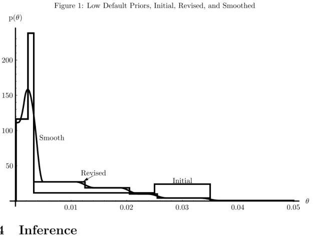
Figure 1 reports the maximum-entropy representation of the prior as initially elicited. This representation, together with the calculation of the implied mean of 0.012, were returned to the expert for discussion and reconsideration. The increase in density moving to the right was not a good reflection of the expert’s assessments. What was desired was a longer right tail but with less density. The expert reassessed the quantiles and added an assessment of the 95th percentile. The results for quan-tiles 0, 0.25, 0.50, 0.75, 0.90, 0.95, 0.99, and 1.0 are 0.0001, 0.00225, 0.0033, 0.0125, 0.0205, 0.0255, 0.035 and 0.05. The resulting ME distribution for the low-default (LD portfolio) is also shown in Figure 1. I have found it useful in this and other ap-plications to assess quantiles and feed back not only the distribution in a graph but the calculated moments. It is very difficult to think about the relationship between tail behavior and moments, especially for higher order moments. Further, feeding back the ME distribution allows the expert to see implications which may not be apparent after a functional form is fit. This method allows the expert to reassess in the light of the implications of quantile assessments for moments. This leads to sharper assessment of quantiles. Finally, various smoothed versions of the ME representation were fed back to the expert. This expert preferred the smooth rep-resentation with a minimal amount of smoothing (h= 600). The resulting smooth prior is also shown in Figure 1.
Figure 1: Low Default Priors, Initial, Revised, and Smoothed Initial p(θ) Revised Smooth θ 0.01 0.02 0.03 0.04 0.05 100 150 200 50
4
Inference
With the likelihood 2 and prior at hand inference is a straightforward application of Bayes rule. Given the distributionp(θ) obtained from our expert, we obtain the joint distribution ofr, the number of defaults, and θ:
p(r, θ) =p(r|θ)p(θ)
from which we obtain the marginal (predictive) distribution of r,
p(r) =
Z
p(r, θ)dθ (11)
and divide to obtain the conditional (posterior) distribution of the parameter of interest θ:
Similarly, if we turn to the model with heterogeneity and dataR = (r1, r2, ...rn) we
find use the likelihood 6 and find the posterior distribution
p(θ|R) = p(R|θ)p(θ)/p(R)
Given the distribution p(θ|r), we might ask for a summary statistic, a suitable estimator for plugging into the required capital formulas as envisioned by Basel Committee on Banking Supervision (2006). A natural value to use is the posterior expectation, θ =E(θ|r). The expectation is an optimal estimator under quadratic loss and is asymptotically an optimal estimator under bowl-shaped loss functions. An alternative, by analogy with the maximum likelihood estimatorθb, is the posterior
mode ·
θ. As a summary measure of our confidence we would use the posterior standard deviation σθ =
q
E(θ−θ)2. By comparison, the usual approximation to the standard deviation of the maximum likelihood estimator is σ
b
θ = q
b
θ(1−θb)/n.
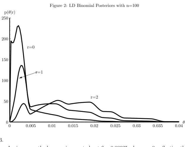
The posterior distributions for n = 100 and r = {0,1,2} are given in Figure 2 for the simple binomial specification. This might correspond to experience with 20 loans/year over the last 5 years, the minimum number of periods required by B2. Zero defaults is the most typical experience for these portfolios with this small sample size.
In this case the likelihood (1− θ)n is smoothly and rapidly decreasing from its mode at θ = 0. The low-θ maximum at about θ = 0.00025 in the posterior for r = 0 is a result of the rapidly declining likelihood combined with the prior which has sharply increasing mass beginning at θ = 0.0001. After that point, the shape of the prior begins to dominate as the likelihood declines smoothly, leading to another, higher, maximum at aroundθ = 0.0025. This shape, which is informative about the relative contribution of the likelihood and the prior, is not attainable under the conjugate prior. Indeed, the extent to which the conjugate prior imposes a straightjacket on information processing is not adequately appreciated. In the
r = 1 case the prior and likelihood largely agree and the posterior has a single maximum. For r = 2 we again see the two maxima, indicating some disagreement between the data and expert information. Summary statistics for these distributions are reported below.
Figure 2: LD Binomial Posteriors with n=100 p(θ|r) r=0 r=1 r=2 θ 0 0.005 0.01 0.015 0.02 0.025 0.03 0.035 0.04 0 100 150 200 250 50 3.
Again we see the low maximum at about θ= 0.00025 whenr = 0,reflecting the strong tendency toward θ= 0 in the data information. In this case that maximum is indeed the mode. For r = 1 and r = 2 the situation is more clear; the data and expert are in reasonably close agreement. The spread out distribution for the
r= 5 case - the density is essentially flat between 0.011 and 0.02 - reflects increased uncertainty when combining the unexpected data and the expert information.
Results for the model with correlated observations are given in Figure 4 for
n = 100 and r ={0,1,2} and observations distributed equally over 5 years There are two cases to consider for r = 2; the case with defaults in the same period and with defaults in different periods. This distinction does not matter of course for the simple Binomial model. Here, the difference in the posterior distributions is trivial and not distinguishable in the graphs so only one case is graphed. The summary statistics are slightly different as reported below. With correlation the data are less informative (note the difference in vertical scale). The unlikely experience of 2 defaults results again in a spread out posterior indicating ambiguity resulting from a disagreement between data and expert information.
Figure 3: LD Binomial Posteriors with n=300 p(θ|r) r=0 r=1 r=2 r=5 θ 0 0.005 0.01 0.015 0.02 0.025 0.03 0.035 0.04 0 100 150 200 250 300 50
Figure 4: LD Correlated Default Posteriors with n=100 p(θ|r) r=0 r=1 r=2 θ 0 0.005 0.01 0.015 0.02 0.025 0.03 0.035 0.04 0 100 150 200 250 50
Figure 5: LD Correlated Default Posteriors with n=300 p(θ|r) r=0 r=1 r=5a r=5b θ 0 0.005 0.01 0.015 0.02 0.025 0.03 0.035 0.04 0 100 150 200 250 300 50
2 extreme cases for 5 defaults, in 5 separate years (graph 5a) and all in the same year (5b). Forr = 0 andr= 1 the posterior densities are concentrated around the unique maximum though both cases exhibit a substantial right tail. For r = 5 a highly unlikely realization for this portfolio segment, the data and prior information differ and this is reflected in spread-out posterior densities.
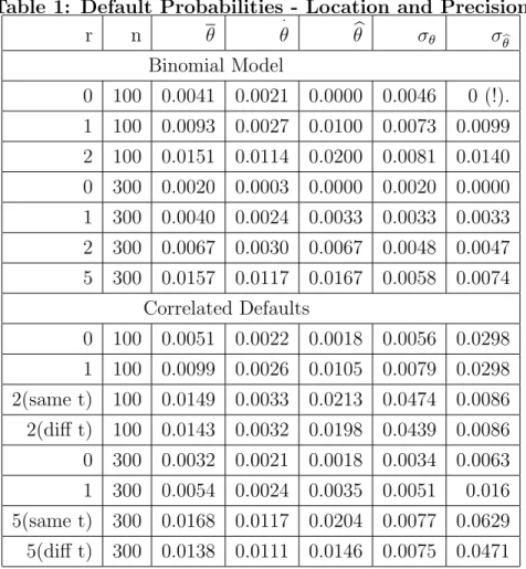
Table 1 gives summary statistics for the prior and posterior distributions. The MLE is given for comparison; clearly this is unacceptable in the zero default case with the Binomial specification, both as a matter of logic and a matter of regulation. The posterior mode for n=300 and zero defaults occurs near the origin, reflecting the combination of the prior with the likelihood rapidly declining from zero (re-call the prior support begins at 0.0001). Thus the mode, sometimes advocated as a computationally convenient alternative to the expectation, does not summarize well the information in the posterior and is probably not a satisfactory alterna-tive to the expectation (though it is more acceptable than the MLE). The MLE is nonzero in the correlated default case even for zero experienced defaults. With the correlated default specification the inference about the long-run default probability tends toward larger values when defaults are clumped within a period relative to evenly distributed defaults. This is indicated not only in the posterior means but
in the posterior modes and the MLEs as well. Note that in all specifications the posterior mean is greater than the mode, reflecting the long right tail in the prior and posterior. The MLE is also greater than the posterior mode except in the case of zero defaults.
Table 1: Default Probabilities - Location and Precision r n θ · θ θb σθ σbθ Binomial Model 0 100 0.0041 0.0021 0.0000 0.0046 0 (!). 1 100 0.0093 0.0027 0.0100 0.0073 0.0099 2 100 0.0151 0.0114 0.0200 0.0081 0.0140 0 300 0.0020 0.0003 0.0000 0.0020 0.0000 1 300 0.0040 0.0024 0.0033 0.0033 0.0033 2 300 0.0067 0.0030 0.0067 0.0048 0.0047 5 300 0.0157 0.0117 0.0167 0.0058 0.0074 Correlated Defaults 0 100 0.0051 0.0022 0.0018 0.0056 0.0298 1 100 0.0099 0.0026 0.0105 0.0079 0.0298 2(same t) 100 0.0149 0.0033 0.0213 0.0474 0.0086 2(diff t) 100 0.0143 0.0032 0.0198 0.0439 0.0086 0 300 0.0032 0.0021 0.0018 0.0034 0.0063 1 300 0.0054 0.0024 0.0035 0.0051 0.016 5(same t) 300 0.0168 0.0117 0.0204 0.0077 0.0629 5(diff t) 300 0.0138 0.0111 0.0146 0.0075 0.0471
5
Prior Distribution II: Mid-Portfolio Assets
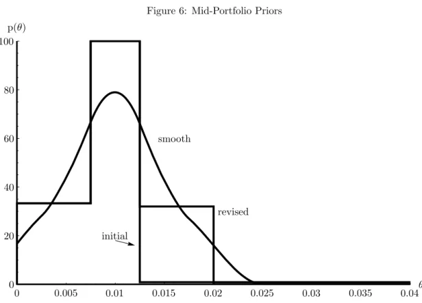
I have asked a different expert to consider a portfolio bucket consisting of loans that might be in the middle of a bank’s portfolio. These are typically commercial loans to unrated companies. If rated, these might be about S&P Baa or Moody’s BBB. The method included a specification of the problem and some specific questions followed by a discussion. Again, our expert found it easier to think in terms of the probabilities directly than in terms of defaults in a hypothetical sample. This may not be so uncommon in this technical area, as practitioners are accustomed to working with probabilities. The mean value was 0.01. The minimum value for the default probability was 0.0001 (one basis point). The expert reported that a value above 0.035 would occur with probability less than 10%, and an absolute upper bound was 0.3. The upper bound was discussed: the expert thought probabilities in the upper tail of his distribution were extremely unlikely, but he did not want to rule out the possibility that the rates were much higher than anticipated (prudence?).Figure 6: Mid-Portfolio Priors initial p(θ) revised smooth θ 0 0.005 0.01 0.015 0.02 0.025 0.03 0.035 0.04 0 100 20 40 60 80
Quartiles were assessed by asking the expert to consider the value at which larger or smaller values would be equiprobable given the value was less than the median, then given the value was more than the median. The median value was 0.01. The former was 0.0075. The latter, the .75 quartile, was assessed at .0125. The expert seemed to be thinking in terms of a normal distribution, perhaps using informally a central limit theorem combined with long experience with this category of assets. Fitting the ME distribution to these values result in a distribution with mean 0.04, reflecting the uniform distribution of mass along the long upper tail. After feedback, the expert reconsidered and added a 0.99 quantile at 0.02. The other assessed quantiles remained the same. The result is to split the long upper tail so that 0.24 of the mass lies between 0.0125 and 0.02, and the remaining 0.01 of the mass is distributed over 0.02 to 0.3. The distribution is shown in Figure 6 together with the smoothed version. The constant density between 0.0075 and 0.0125 reflects two assessments; the 25th and 75th percentile points are symmetric around the median. This expert preferred more smoothing, choosing h= 200.
Binomial
Correlated
Figure 7: Mid-Portfolio Posteriors p(θ) θ 0 0.005 0.01 0.015 0.02 0.025 0.03 0.035 0.04 0 100 150 200 250 50
6
Inference
The mid-portfolio applications will typically have a larger sample size as well as a higher default probability than the low-default application. Thus it is more difficult to study a ”typical” sample, as above. Further, the larger sample and higher ex-pected default rate may support the correlated default specification in which case the pattern of defaults over time is important and it is difficult to think of typical samples. We construct a hypothetical bucket of mid-portfolio corporate bonds from S&P-rated firms in the KMV North American Non-Financial Dataset. Default rates were computed for cohorts of firms starting in September 1993 and running through September 2004. In total there are 2197 asset/years of data and 20 defaults, for an overall empirical rate of 0.00913. The posterior densities for the Binomial and correlated models are shown in Figure 7.
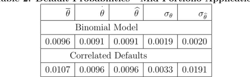
The densities have a single maximum and the default probability is well deter-mined. The model allowing correlated defaults does not give as sharp an inference of course, but seems to tell the same story. The Binomial model gives slightly lower estimates of the long-run default probability than the model with correlated de-faults. In this sample, the posterior mode and the MLE coincide. The posterior
expectation is greater than the MLE, reflecting the influence of the long right tail. The expert information is more important in the correlated default model, as re-flected in the difference between the posterior standard deviation and the standard deviation of the MLE (note that these are often compared but in fact have quite different interpretations).
Table 2: Default Probabilities - Mid-Portfolio Application
θ · θ θb σθ σ b θ Binomial Model 0.0096 0.0091 0.0091 0.0019 0.0020 Correlated Defaults 0.0107 0.0096 0.0096 0.0033 0.0191
We estimated this model using direct numerical integration (with MathematicaTM 6.0). Estimation of much more complicated models is now straightforward us-ing Markov Chain Monte Carlo (MCMC) and related procedures (see Robert and Casella (2004) and Geweke (2005)).
7
Inference for minimum required capital
The default probabilities are used to calculate minimum capital requirements under Basel II. To this end, an estimate is plugged into a formula given by the authorities Basel Committee on Banking Supervision (2006), p. 64 as
K(θ) = [LGD× Φ[(1−ρ(θ))−1/2× Φ−1(θ) + (ρ(θ)/(1−ρ(θ)))1/2× Φ−1(0.999)]
−θ×LGD]×(1−1.5×b)−1× (1 + (M −2.5)× b)
whereb= (0.11852−0.05478× ln(θ))2 is a maturity adjustment, ρ(θ) from 5 is an adjustment for correlation among defaults, LGD is loss given default andK(θ) is the capital requirement (a fraction). In our calculations we take LGD=1. In practice LGD is another parameter to be estimated and inserted into the equation. Note that the capital requirement function exhibits a singularity atθ =2.9272x10⁻⁶.The limit from the right is +∞, from the left -∞. It is unlikely that this would come up in ordinary calculations to the usual levels of numerical accuracy, but it is something to be aware of since extensive simulations are sometimes used in applications and
a low-probability realization could dramatically influence results. In practice, there is a lower bound of 0.0003 on the estimate of θ to be used in the capital formula (Basel Committee on Banking Supervision (2006), p. 67). In the calculations below we impose the restriction, so the actual capital function isK(0.0003) forθ <0.0003 and K(θ) otherwise. This function is not concave for low values of θ,although it is concave for values above three basis points.
Although the regulations specify that an estimate of the default probability will be plugged into the formula, we have more than a point estimator available, we have a complete probabilistic description of the uncertainty in θ. This implies a probability distribution for required capital K(θ) by a simple change of variable. If the formula is viewed as relevant for the true default probability, then it may arguably be more appropriate to calculate capital by EK(θ) than by K(θ∗) where
θ∗ is some point estimate of θ. The natural estimate to use is E(θ), so the issue is whether to use EK(θ) or K(E(θ)). Since the bulk of the mass of the distribution ofθ occurs where K is concave, the first calculation gives smaller values of required capital. The implications of this consideration for the choice of portfolio buckets are explored by Kiefer and Larson (2004) from a sampling point of view.
In the mid-portfolio application we have K(E(θ)) = 0.1617 and EK(θ) = 0.1603 in the Binomial case and K(E(θ)) = 0.1681 and EK(θ) = 0.1651 in the correlated default case. The larger difference in the correlated case reflects the higher uncertainty. Apparently banks desiring lower capital positions would prefer increased uncertainty for this calculation, though for internal business analytics (for example, in pricing credit) increased precision is naturally preferred. This perverse incentive points to the need to think clearly about the losses associated with mis-specifying minimum regulatory capital. It is likely that a quadratic loss function, or something quite like quadratic loss, leading to the mean as an optimal estimator, is inappropriate here. Perhaps losses associated with getting capital too low, leading to increased risk of default by the bank, is substantially worse than getting capital too high, leading to reduced profits by the bank. Partial evidence on this score is provided by the fact that banks, who may favor profits over safety more than supervisors, routinely hold more than the minimum required capital.
We address this possibility by considering loss functions of the form bH(k − k0)−aH(k0 −k) where H(w) is the Heaviside function H(w) = 0 for w < 0 and H(w) = 1 for w ≥ 0; a piecewise linear loss function. Minimizing expected loss gives capital K = F−1(a/(a+b)) where F is the posterior distribution function.
We expect that a > b, though quantitative considerations of the loss are difficult and are not given in B2. Fora/(a+b) = (1/2,2/3,3/4) the optimal values of capital are (0.165, 0.173, 0.178) in the correlated default case and (0.161, 0.166, 0.168) for the Binomial specification. Here the gains associated with increased precision are clear.
8
Conclusion
I have considered inference about the default probability for a low-default portfolio bucket and for a mid-portfolio bucket. For low-default portfolios or for very new as-sets there is unlikely to be substantial data information about the long-run default rate. Nevertheless banks must make credit allocation decisions and those banks governed by the Basel II regulations must estimate default probabilities and justify their estimation procedures to supervisors. Expert judgment is expected though the B2 regulations do not explicitly recommend quantification of expert information in probability terms. If this information can be quantified in probabilities, then the information can be combined coherently using the ordinary properties of probabil-ities. This leads to a tremendous simplification of the numerous and difficult ad hoc considerations that lead to situation-specific solutions to the inference prob-lem. An industry expert with long experience with this portfolio segment agreed to the elicitation. The expert was able to give probabilities for ranges of the default probability, specifying various percentiles. A maximum entropy approach gave a statistical representation of the probabilities with as little additional information as possible. This was a useful device for feeding back implications to the expert and inducing revisions in the elicited probabilities. A smoothed version of the final elicited maximum entropy distribution provided the prior for a Bayesian analysis. In the low default case, the number of defaults will be small with high probability. I reported results for sample sizes of 50 and 300, representing the likely range of data. Though these data sets were hypothetical, they are typical and the results are use-ful, not least because the embarrassing and unacceptable estimate of a zero default probability based on the MLE does not arise. In a second application, I interviewed an expert with wide experience in mid-portfolio assets. The same procedure was followed: an initial elicitation led to a maximum-entropy distribution, with impli-cations fed back to the expert for consideration. Then, a smoothed version of the final elicitation was used in an analysis. In this application it is more difficult to
specify a typical dataset. A portfolio consisting of mid-portfolio corporate bonds was constructed and used in the application.
Two specifications were used for the likelihood function, both consistent with the Basel II model. The first is a simple Binomial, probably the model in widest use in practice. This model for defaults is consistent with a model in which asset values are iid and default occurs when a (lower) threshold is crossed. An extension in which asset values follow a single factor model consisting of a period-specific shock common to all assets in the portfolio bucket and an idiosyncratic shock is consistent with the B2 capital model. This is a richer specification in which period-specific default rates are essentially inputs to estimating a long-run default rate. As a consequence, inferences in this expanded model are much less sharp since the data are less informative. Thus the expert information is particularly valuable. Both models were estimated for both the low-default application and the mid-portfolio application. Implications for minimum required capital based on the B2 formulas and the posterior distribution are explored. At the validation stage, modelers can be expected to have to justify the likelihood specification and the representation of expert information. Methods for validation of Bayesian procedures are yet to be developed.
In this and related applications the econometrician faces the dual chore of model-ing the data distribution with a specification of a statistical distribution and mod-eling expert information with a statistical distribution. Adding the latter task substantially increases the range of applicability of econometric methods. This is clearly an area for further research.
References
Basel Committee on Banking Supervision (2005): “Basel Committee
Newsletter No. 6: Validation of Low-Default Portfolios in the Basel II Frame-work,” Discussion paper, Bank for International Settlements.
(2006): “International Convergence of Capital Measurement and Capital Standards: A Revised Framework, Comprehensive Version,” Bank for Interna-tional Settlements.
British Banking Association, London Investment Banking Association and In-ternational Swaps and Derivatives Association, Joint Industry Working Group.
Berger, J. O. (1980): Statistical Decision Theory: Foundations, Concepts and
Methods. Springer-Verlag.
Chaloner, K. M., and G. T. Duncan (1983): “Assessment of a Beta Prior
Distribution: PM Elicitation,” The Statistician, 32(1/2, Proceedings of the 1982 I.O.S. Annual Conference on Practical Bayesian Statistics), 174–180.
Cover, T. M., and J. A. Thomas (1991): Elements of Information Theory.
John Wiley & Sons.
Csiszar, I.(1975): “I-divergence Geometry of Probability Distributions and
Min-imization Problems,” The Annals of Probability, 3, 146–158.
Das, S. R., D. Duffie, N. Kapadia, and L. Saita(2007): “Common Failings:
How Corporate Defaults are Correlated,” Journal of Finance, 62, 93–117.
DeGroot, M. H. (1970): Optimal Statistical Decisions. McGraw-Hill.
Dufour, J.-M., F. Jouneau-Sion, and O. Torrs (2007): “Testability and
methods of moments in nonparametric and semiparametric models,” Discussion paper, McGill University.
Garthwaite, P. H., J. B. Kadane, and A. O’Hagan (2005): “Statistical
Methods for Eliciting Probability Distributions,” Journal of the American Sta-tistical Association, 100, 780–700.
Gavasakar, U. (1988): “A Comparison of Two Elicitation Methods for a Prior
Distribution for a Binomial Parameter,” Management Science, 34:6, 784–790.
Geweke, J. (2005): Contemporary Bayesian Exonometrics and Statistics. New
York: John Wiley & Sons.
Gordy, M. B.(2003): “A Risk-Factor Model Foundation for Ratings-Based Bank
Capital Rules,” Journal of Financial Intermediation, 12, 199–232.
Jaynes, E. T.(2003): Probability Theory: The Logic of Science. New York:
Kadane, J. B., J. M. Dickey, R. L. Winkler, W. S. Smith, and S. C. Peters (1980): “Interactive Elicitation of Opinion for a Normal Linear Model,”
Journal of the American Statistical Association, 75(372), 845–854.
Kadane, J. B., and L. J. Wolfson (1998): “Experiences in Elicitation,” The
Statistician, 47(1), 3–19.
Kiefer, N. M. (forthcoming): “Default Estimation for Low Default Portfolios,”
Journal of Empirical Finance, OCC Working Paper.
Kiefer, N. M., and C. E. Larson (2004): “Evaluating Design Choices in
Eco-nomic Capital Modeling: A Loss Function Approach,” in Economic Capital: A Practitioner Guide, ed. by A. Dev, chap. 15. Risk Books, London.
Nickell, P., W. Perraudin, and S. Varotto (2000): “Stability of Rating
Transitions,” Journal of Banking and Finance, 24, 203–227.
Nyarko, Y.,and A. Schotter(2002): “An Experimental Study of Belief
Learn-ing UsLearn-ing Elicited Beliefs,” Econometrica, 70(3), 971–1005.
OCC, FRS, FDIC, and OTS(2007): “Risk-Based Capital Standards: Advanced
Capital Adequacy Framework–Basel II; Final Rule,” Federal Register, 72(235), 69288–69445.
O’Hagan, A., C. E. Buck, A. Daneshkhah, J. R. Eiser, P. Garthwaite, D. J. Jenkinson, J. E. Oakley, and T. Rakow (2006): Uncertain
Judge-ments: Eliciting Experts’ Probabilities. Chichester: John Wiley & Sons.
Pluto, K., and D. Tasche (2005): “Thinking Positively,”Risk, August, 72–78. Robert, C., and G. Casella (2004): Monte Carlo Statistical Methods (2nd
edition). New York: Springer-Verlag.
Schuster, E. F. (1985): “Incorporating support constraints into nonparametric
estimators of densities,” Communications in Statistical Theory and Methods, 14, 1123–1136.