J
ournal of the
A
ssociation for
I
nformation
S
ystems
Research Paper ISSN: 1536-9323
An Extensive Examination of Regression Models with a
Binary Outcome Variable
Suneel Babu Chatla
Institute of Service Science National Tsing Hua University, Taiwan
Galit Shmueli
Institute of Service Science National Tsing Hua University, Taiwan
Abstract:
Linear regression is among the most popular statistical models in social sciences research, and researchers in various disciplines use linear probability models (LPMs)—linear regression models applied to a binary outcome. Surprisingly, LPMs are rare in the IS literature, where researchers typically use logit and probit models for binary outcomes. Researchers have examined specific aspects of LPMs’ but not thoroughly evaluated their practical pros and cons for different research goals under different scenarios. We perform an extensive simulation study to evaluate the advantages and dangers of LPMs, especially with respect to big data, which is now common in IS research. We evaluate LPMs for three common uses of binary outcome models: inference and estimation, prediction and classification, and selection bias. We compare its performance to logit and probit under different sample sizes, error distributions, and more. We find that coefficient directions, statistical significance, and marginal effects yield results similar to logit and probit. In addition, LPM estimators are consistent for the true parameters up to a multiplicative scalar. This scalar, although rarely required, can be estimated assuming an appropriate error distribution. For classification and selection bias, LPMs are on par with logit and probit models in terms of class separation and ranking and is a viable alternative in selection models. LPMs are lacking when the predicted probabilities are of interest because predicted probabilities can exceed the unit interval. We illustrate some of these results by modeling price in online auctions using data from eBay.
Keywords: Linear Regression, Linear Probability Model, Binary Outcome, Selection Bias, Estimation, Inference, Prediction, Big Data, Logit, Probit.
Kenny Cheng was the accepting senior editor. This article was submitted on February 17, 2016, and went through two revisions.
"Entities should not be multiplied unnecessarily.” (Occam’s razor)
1
Introduction and Motivation
Binary outcomes are common in the information systems (IS) literature. Among models for a binary dependent variable, logistic and probit regression models are the most commonly used in IS. These models are used for three main purposes:
1. Inference and estimation: estimating and testing the effect of covariates of interest on a binary outcome.
2. Classification: predicting the class or probability for new records.
3. Selection bias: estimating the selection model in propensity score matching and in the first stage of 2SLS models.
Among the many empirical IS studies that model binary dependent variables, the great majority use logistic regression for inference (e.g., Susarla, Subramanyam, and Kargade’s (2010) model renewal of outsourcing contracts (yes/no); Rishika, Kumar, Janakiraman, and Bezawada’s (2013) model social media participation; Asvanund, Clay, Krishnan, and Smith’s (2004) model song availability in P2P networks (available/unavailable); and Hui, Teo, and Lee’s (2007) model disclosure of private information by online users (yes/no)), logistic regression for selection bias using propensity score matching (e.g., Mithas & Krishnan, 2009; Rishika et al., 2013), and probit regression for selection bias using 2SLS (e.g., Kuan, Hui, Prasarnphanich, & Lai, 2015; Gopal & Koka., 2012; Kwon & Johnson., 2014; Liu, Brass, & Chen, 2014). A linear probability model (LPM)—linear regression model applied to a binary dependent variable—is an alternative to logistic and probit regression models.
Notation: assume that we have 𝑛 observations and 𝑝 independent variables. We define the dependent variable 𝑍𝑛×1= [
𝑧1
𝑧2
⋮ 𝑧𝑛
], where 𝑧𝑖 ∈ {0,1}; design matrix 𝑿𝒏×(𝒑+𝟏)=
[ 𝒙𝟏𝑻 𝒙𝟐 𝑻 ⋮ 𝒙𝒏𝑻] , where 𝒙𝒊𝑻= [𝟏 𝒙𝒊𝟏𝒙𝒊𝟏… 𝒙𝒊𝒑], 𝑖 =
1,2, … , 𝑛; parameter vector 𝛽(𝑝+1)×1; and error term 𝜀𝑛×1= [
𝜀1
𝜀2
⋮ 𝜀𝑛
]. The LPM model is given by:
𝑍 = 𝑿𝛽 + 𝜀, (1)
or, using observation specific notation, 𝑧𝑖= 𝒙𝒊𝑻𝜷 + 𝜀𝑖. The model is estimated using ordinary least squares
(OLS).
LPMs are common in disciplines such as economics and political science for each of the three goals mentioned earlier: inference (e.g., McGarry, 2000; Fairlie & Sundstrom, 1998; Betts & Fairlie, 2001; Klaassen & Magnus, 2001; Lukashin, 2000), classification (e.g., Heckman & Snyder, 1996), and selection bias (Olsen, 1980). Yet, LPMs are rare in the IS literature.
1.1
LPMs in the Information Systems Literature
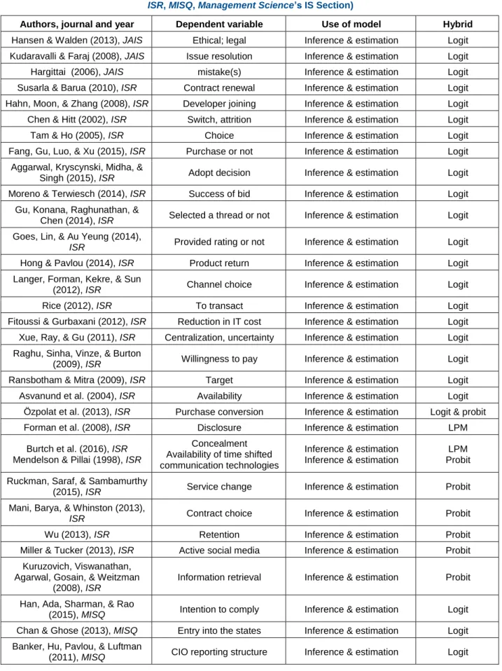
We conducted a full-text search1 of binary dependent variable models in the journals Information Systems
Research (1990 to September 2016), MIS Quarterly (1977 to September 2016), Journal of the Association for Information Systems (2003 to September 2016), and the IS section of Management Science (1954 to September 2016). We found 92 papers that modeled a binary dependent variable, but only eight of them used a LPM. For example, Burtch, Ghose, and Wattal (2016) used a LPM to avoid the incidental parameter problem that the logit models have. Schlereth and Skiera (2017) considered a LPM to obtain the rankings for the choice probabilities as quickly as possible and because LPMs are very fast. Miller and Tucker (2009) used a LPM to study the diffusion of EMR technology using data from 2910 hospitals. Forman, Ghose, and Wiesenfeld (2008) used a LPM to model the presence of identity-disclosure information in online reviews present/absent) applied to over 160,000 book reviews on Amazon.com. Forman, Ghose, and Goldfarb
1 We performed a full text search using EBSCO with keywords “linear probability model”, “regression”+”binary”,
(2009) used a LPM to model data from Amazon.com on the top-selling books for 1,497 unique locations in the United States for 10 months in order to evaluate the effect of customers’ locations on their online/offline shopping choice. Adjerid, Acquisti, Teland, Padman, and Adler-Milstein (2015) used a LPM for both cross sectional (survey) and panel (6 years) datasets. Ceccagnoli, Forman, Huang, and Wu (2012) used a LPM to model a panel dataset on 1,210 small independent software vendors (ISV) over the 1996-2004 period to study how participation in an ecosystem partnership improves the business performance of the small ISVs. These five papers used LPMs for inference. Table 1 summarizes our literature search results, and Table A1 presents them in more detail.
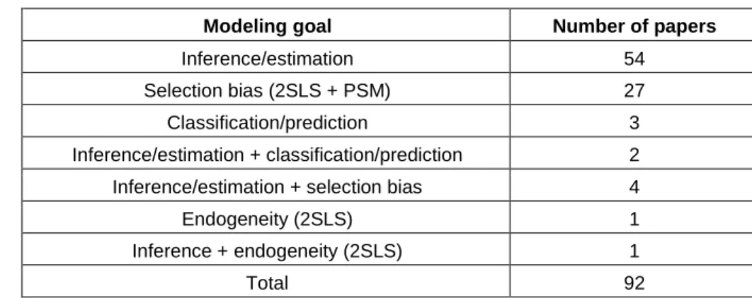
Table 1. Summary of IS Literature Survey of Binary Outcome Models
Modeling goal Number of papers
Inference/estimation 54 Selection bias (2SLS + PSM) 27 Classification/prediction 3 Inference/estimation + classification/prediction 2 Inference/estimation + selection bias 4 Endogeneity (2SLS) 1 Inference + endogeneity (2SLS) 1
Total 92
1.2
LPM in Big Data
In the realm of big data where large samples are available, researchers have claimed that LPMs produce qualitatively similar results to both logistic and probit regression models (Gordon, Lin, Osberg, & Phipps, 1994; Betts & Fairlie, 2001). Large samples are now becoming popular in IS studies, and many IS researchers have begun to focus on working with big data. Thought leaders and editors of leading IS journals see much reason for optimism regarding big data’s impact on the IS discipline (Abbasi, Sarker, & Chiang, 2016; Agarwal & Dhar, 2014). Advances in technology have brought us the ability to collect, transfer, and store large data sets. Thanks to this, a growing number of empirical studies published in information systems and related disciplines now rely on very large samples (Lin, Lucas, & Shmueli, 2013). Among those studies, some have a binary outcome. For example, Özpolat, Gao, Jank, and Viswanathan (2013) used a logit model to study the presence/absence of online trust seals using over 9000 online shopping sessions; Overby and Jap (2009) analyzed over 100,000 used vehicles in the wholesale automotive market using probit models to study virtual versus physical vehicle presentation by the seller and physical versus virtual presence of the buyer. Asvanund et al. (2004) use a probit regression to model song availability in a P2P network for over 160,000 songs. Only a single large-sample binary-outcome paper used a LPM (Forman et al., 2008). Therefore, we are interested in evaluating the performance of a LPM against its alternatives also in the case of large samples.
1.3
Goal of This Study
In this paper, we examine the performance of LPMs with respect to large samples. We start by describing the advantages and weaknesses of LPMs based on examining the literature on them in different areas. Since the literature is inconclusive, we examine and evaluate LPMs’ strengths and weaknesses through an extensive simulation study.
We consider and examine LPMs’ components that one uses for inference and estimation, classification and prediction, and selection bias: coefficients (in terms of bias and consistency) and fitted/predicted values. We then examine how these components affect the three goals. In doing so, we provide researchers and practitioners with an understanding of when LPMs are useful, when they are not, and what they should expect under different scenarios.
The paper proceeds as follows: in Section 2, we describe the criticisms, controversies, and justifications surrounding using LPMs as they appear in the extant literature. In Section 3, we provide theoretical results regarding consistency of the estimators, marginal effects, predicted values, and classification. In Section 4, we describe the simulation study (in which we compared LPMs with logit and probit models in terms of coefficient estimation, significance, prediction, and selection models) and its results. In Section 5, we
illustrate some of these results using a real dataset on online auctions. In Section 6, we summarize our results, offer directions for future research, and conclude the paper.
2
Criticism of, Controversy about, and Justification for LPMs in the
Literature
2.1
Criticisms of LPMs
Estimating LPMs using ordinary least squares (OLS) has four main problems (Maddala, 1986):
1. Non-normal error term: for a binary dependent variable, the error term εi can only take two
values:εi = 1 − xi T
β if zi = 1 and εi = −xi T
β if zi= 0. Hence the normality assumption cannot
be valid.
2. Non-constant error variance: the variance for a binary outcome is given by σi2 =E[zi](1 − E[zi]). Since E[zi] is a function of Xi, the variance varies for different levels of X
and, thus, the homoscedasticity assumption is violated.
3. Constraints on the response function: since E[zi] represents probabilities, they should be
constrained between 0 and 1 (i.e., 0 ≤E[zi]≤ 1). However, the LPM does not institute this
constraint.
4. Functional form: since the model is linear, a unit increase in one of the covariates of 𝑋 (say, 𝑥𝑘) is interpreted as a constant change of 𝛽𝑘 in the probability of an event while holding the
remaining covariates constant. The magnitude change should be constant regardless of the current value of 𝑥𝑘. In many applications, however, this is unrealistic. In general, when the
outcome is a probability, it is reasonable that the effects of covariates will diminish as the predicted probability approaches 0 or 1. Long and Freese (2006) states that this problem is the most serious one with LPMs.
Given these four issues, conventional advice (Gordon et al., 1994) suggests using generalized linear models (GLMs) with logit or probit link functions to overcome all four issues. By choosing a sigmoidal curve or an inverse normal cumulative distribution function (ICDF) as a functional form, one overcomes all of the above limitations. The logit and probit links are symmetric and can produce diminishing effects as the probability approaches 0 or 1, and they mostly differ from each other at the tails. For small samples, both techniques produce similar results, but, as the sample size increases, the differences are more evident (Gordon et al., 1994). For an asymmetric link function, the literature suggests using a complementary log-log function.
Since one does not encounter the above four problems with logit or probit models, the latter have become the common choice for modeling binary outcomes. While there is an additional cost of computational complexity when using logit/probit models, that cost is practically negligible due to the advancements in computational power.
2.2
Debate about the Criticism in the Literature
The statistical arguments against using linear regression with a binary dependent variable are not as decisive as research has often claimed (Hellevik, 2009). Several papers discuss the impact of each of the four issues in Section 2.1 on inference and prediction, which makes the criticism of LPMs a more debatable issue.
In terms of non-normal error terms (challenge #1), OLS provides estimators that are asymptotically normal under quite general conditions even if the distribution of the error terms is far from normal. With a large sample, this challenge is, therefore, mute (Aldrich & Nelson, 1984; Long & Freese (2006).
The non-constant error variance (challenge #2) is of no consequence for the regression coefficient, but the uncertainty estimate for the coefficient and, thus, the test of significance is affected (Hellevik, 2009). In studies interested in inference, the literature suggests substituting OLS estimation with weighted least squares (WLS) to estimate the model. This two-stage procedure first produces fitted values 𝑧
̂
𝑖 = 𝑥𝑖𝑇𝛽̂
(i=1,…,n) from the OLS estimation and then re-estimates the model using WLS with weights 𝑤𝑖 =
The implication of the unconstrained response function (challenge #3) is that predicted values, which reflect probabilities, are not constrained to the unit interval. Friedman et al. (2009, p. 103) comment about an unconstrained response function’s impact on classification as follows: “these violations themselves do not guarantee that this approach will not work, and in fact on many problems it gives similar results to more standard linear methods for classification”. In other words, when one uses the probabilities for classification, one is interested only in comparing P(𝑧𝑖=1) to P(𝑧𝑖=0) and classifying the observation to the
class with the higher probability.
When one focuses on the probability itself, then values beyond the unit interval are problematic. The ad hoc solution to this problem is simply replacing values above 1 with 1 and values below 0 with 0 (Mukras, 1993). As Figure A5 shows, whenever LPMs produce unbounded predictions, both logistic and probit models produce predictions equal exactly to 1 or 0. Hence, it is indeed reasonable to replace the unbounded predictions with either 0 or 1. Unbounded predictions can also cause problems while calculating weights for WLS (for addressing challenge #2). To solve the problem of calculating weights for WLS, researchers suggest replacing predictions above 1 with 0.999 and predictions below 0 with 0.001 (Aldrich & Nelson, 1984), which guarantees positive weights as WLS requires. In general, the percentage of unbounded predictions produced by LPMs is small, and they mainly happen due to outliers in the data (high leverage and influential observations). Hence, rounding off predictions would actually improve the LPM standard errors, which both logistic and probit models do by default.
When LPMs produce many unbounded predictions, it might indicate either an underspecified model (Friedman et al. 2009) or LPMs’ inadequacy. Unbounded predictions will affect both inference and prediction. The functional form issue (challenge #4), which is based on the claim that the effect of covariates on the probability more realistically diminishes near 0 or 1 rather than behaves linearly, relates more directly to LPMs’ inadequacy. One can base these claims on either theoretical considerations or empirical tests. For example, if there are many unbounded predictions, then a linear specification may not be appropriate. However, there is no empirical evidence on what percentage of unbounded predictions one can use to decide about whether to use a LPM.
2.3
Justification for the LPM
In their book Mostly Harmless Econometrics, Angrist and Pischke (2008) discuss LPMs’ theoretical and practical advantages compared to GLMs such as logistic and probit models in terms of linking inference with causality and causally interpreting regression coefficients. They conclude (p. 107):
While nonlinear models may fit the [conditional expectation function] more closely than a linear model, when it comes to marginal effect this probably matters little…. Nonlinear models require a number of decisions along the way (e.g., the weighting scheme, derivatives vs. finite differences), while OLS is standardized. Nonlinear life also gets considerably more complicated when we work with instrumental variables and panel data. Finally, extra complexity comes into the inference step as well, since we need standard errors for marginal effects.
Hellevik (2009) further notes that one cannot apply loglinear measures in causal analyses since they do not accurately describe (multivariate) associations.
Because typically one does not know the underlying true model, one can choose a model—whether logistic, probit, or linear probability model—based only on an approximation. Thus, one might ask how choosing the “wrong” model harms the results. Angrist and Pischke (2012, July 09) state:
The LPM won’t give the true marginal effects from the right nonlinear model. But then, the same is true for the wrong nonlinear model! The fact that we have a probit, a logit, and the LPM is just a statement to the fact that we don’t know what the “right” model is. Hence, there is a lot to be said for sticking to a linear regression function as compared to a fairly arbitrary choice of a non-linear one!
Li and Duan (1989) show that one can still obtain consistent estimators for the regression parameters even under link violation as long as the covariates are spherically distributed (e.g., follow a normal distribution) along with some other conditions. However, when the data are far from normally distributed (e.g., heavily skewed), the coefficients estimated from either probit or logit models will differ from the true values.
In some cases, only LPMs allow model estimation. Specifically, one can estimate coefficients of some dummy variables in a LPM but not in a logistic or probit regression model (Anderson, 1987; Caudill, 1987).
For example, one cannot estimate observation-specific dummies and group-specific dummies, where all members of the group belong to the same class, with either logit or probit models. While this phenomenon is rare in cross sectional studies, it is quite common in panel data studies. This phenomenon is also probably one of the reasons behind why many panel studies choose LPM over either logit or probit models (Forman et al, 2008; Adjerid et al., 2015); with a LPM, one can estimate these effects quite comfortably. Similarly, both logit and probit run into problems when a complete or quasi-separation exists in the data.
Multiple authors point to LPMs’ interpretational advantage over non-linear models, especially when the model includes interaction terms. McGarry (2000) appeals to the ease of interpreting estimated marginal effects. Fairlie and Sundstrom (1998) prefer LPMs due to the ease with which one can interpret coefficients. Wooldridge (2010, p. 455) also advocates using a LPM when one seeks estimation or inference:
If the main purpose is to estimate the partial effect of [the covariate] on the response probability, averaged across the distribution of [the covariates], then the fact that some predicted values are outside the unit interval may not be very important.
With a large sample, researchers have claimed LPMs to produce qualitatively similar results to both logistic and probit regression models (Gordon et al., 1994; Betts & Fairlie, 2001). Existing research on selection bias showcases the successful use of LPM. The two-stage least squares (2SLS) approach for selection bias comprises the following two models:
1. Selection model: 𝑆∗𝑛×1 = 𝑊𝑛×(𝑘+1)𝛾 + 𝜔𝑛×1
,
where 𝑆∗ is latent and we observe 𝑆 = 1 if 𝑆∗ ≥0and 𝑆 = 0 otherwise. We assume there are only 𝑚 < 𝑛 observations with 𝑆 = 1.
2. Outcome model: 𝑌𝑚×1 = 𝑋𝑚×(𝑝+1)𝛽 + 𝜀𝑚×1, where 𝑌 is observed only if 𝑆 = 1. While it is not
uncommon to use the same set of covariates in both the models (i.e., 𝑊 = 𝑋), it is preferable to use at least one different covariate than the covariates in outcome model.
If we assume both errors (𝜔, 𝜀) follow a bivariate normal distribution, then we can estimate the above model using ordinary likelihood based methods that require solving an iterative algorithm. Heckman (1979) paved the way for the prevalence of methods for correcting sample selection bias. Heckman simplified the above complex Maximum likelihood (ML)-based estimation procedure into two simple steps: 1) estimate the selection model with a probit model and calculate the inverse Mills ratio (IMR= ∅(Wγ̂)
Φ(Wγ̂),
where Φ is the standard normal density and Φ is the standard normal CDF); and 2) estimate the outcome model, which includes the IMR as an extra covariate to control for selection bias. Olsen (1980) further simplified the estimation by replacing the probit selection model with a LPM and using the fitted values (Wγ̂ − 1)) directly in the outcome model as an extra predictor. Olsen’s LPM approach requires that the conditional expectation of 𝜀|𝜔 is linear in 𝜔, and this assumption is more flexible than the bivariate normality required for Heckman’s approach. While some researchers have criticized Olsen’s approach for using a LPM, others have showed that the two approaches yield identical results (Wooldridge, 2010; Olsen, 1980; Angrist & Pischke, 2008).
In the context of endogeneity, when one uses 2SLS for handling a binary endogenous variable, the advantage of using LPM in the first stage is that plugging the first-stage fitted values into the second stage regression results in consistent 2SLS estimates. Using a nonlinear model in the first stage to increase the 2SLS estimate efficiency requires special care to avoid “forbidden regressions” (typically done by treating the first-stage fitted values as instruments). Angrist and Pischke (2008, p. 191) conclude: “Use of a nonlinear plug-in first-stage may not do too much damage in practice—a probit first-stage can be pretty close to linear—but why take a chance when you don’t have to?”.
Lastly, another advantage of LPMs is computational: least squares estimation is computationally cheaper than the ML method used for estimating logistic or probit regression models. ML relies on an iterative algorithm that is sequential in nature and, therefore, difficult to parallelize (Yahav, Shmueli, & Mani, 2016). This computational advantage is not a big concern given today’s computing power. However, there are situations where even a small gain in time is meaningful.
3
LPMs for Estimation and Inference vs. Fitted and Predicted Values
Proponents and critics of LPMs typically rest their claims on theoretical or practical arguments that affect statistical inference, parameter estimation, and prediction. Statistical significance and parameter
estimation are relevant to the goals of inference, while prediction is relevant to the goals of classification and selection bias. Therefore, we distinguish between the scenarios of explanatory modeling where one focuses on parameter estimation and statistical inference and predictive modeling where one focuses on predicted values (Shmueli, 2010; Shmueli & Koppius, 2011). For example, some studies show that, in large samples, LPMs produce results “similar” to logistic and probit regression models. Researchers sometimes measure similarity in terms of prediction accuracy (Gordon et al., 1994) and, at other times, in terms of statistical significance (Hellevik, 2009).
Given the two different contexts and the different uses of binary outcome models, we examine and summarize results regarding the following quantities: coefficient bias, marginal effects, fitted/predicted probabilities, and classifications.
3.1
Formulation of the Binary Outcome Scenario
Coefficient bias and interpretation are major concerns when one seeks parameter estimation. In the statistics literature, one possible way to motivate binary variable models is to assume that there exists an underlying latent continuous variable that has been discretized so that one only observes the discretized (binary) version. Assume the true underlying model with continuous dependent variable is as follows:
𝑌𝑛×1 = 𝑋𝑛×(𝑝+1)𝛽(𝑝+1)×1+ 𝜀𝑛×1, 𝜀𝑖~𝑓
(
0, 𝜎2)
, (2)where 𝑓 (.) = any symmetric continuous density and Y is a latent continuous variable, we observe only: 𝑍 = {1, 𝑖𝑓 𝑌 > 0
0, 𝑖𝑓 𝑌 < 0 (3)
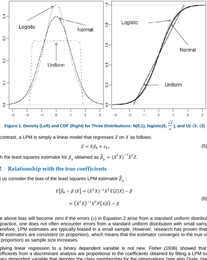
Based on the error distribution f(.), we select the model to estimate the parameters of interest. For simplicity, let us consider f = {uniform, logistic, normal}. Figure 1 illustrates the similarity of these three distributions when they have mean zero and variance equal to one. Ideally, one would fit a probit model if the errors arise from a standard normal distribution and a logistic regression if the errors arise from a standard logistic distribution. Although not as popular, one would fit a linear probability model if the errors arise from a standard uniform distribution. From Equations 2 and 3, we can write:
𝐸[𝑍|𝑋] = ℱ(𝑋𝛽), (4)
where ℱ (.) is the cumulative distribution function (CDF) for the density 𝑓 (.) in Equation 2. Both logistic (logit) and probit models assume the random variable 𝑍 follows a Bernoulli distribution with the probability defined in Equation 4, and we estimate parameters using MLE. It is well known that, under some regularity conditions, the ML estimators are consistent (𝛽
̂
𝑝
→
𝛽). However, although we estimate Equation 4 to retrieve the estimates for the original model in Equation 2, one has to interpret the resulting coefficients completely differently from how one should interpret the original coefficients due to 𝑌’s unobserved nature and the fact that one draws interpretations with respect to the observed binary 𝑍.Figure 1. Density (Left) and CDF (Right) for Three Distributions: N(0,1), logistic(0,√𝟑
𝝅 ), and U(-√3, √3)
In contrast, a LPM is simply a linear model that regresses 𝑍 on 𝑋 as follows:
𝑍 = 𝑋𝛽𝑏+ 𝜀𝑏
,
(5)with the least squares estimator for 𝛽𝑏 obtained as 𝛽
̂
𝑏= (𝑋𝑇𝑋)−1𝑋𝑇𝑍.3.2
Relationship with the true coefficients
Let us consider the bias of the least squares LPM estimator 𝛽
̂
𝑏 : 𝐸[𝛽̂𝑏− 𝛽 |𝑋] = (𝑋𝑇𝑋)−1𝑋𝑇𝐸[𝑍|𝑋] − 𝛽=
(
𝑋𝑇𝑋)
−1𝑋𝑇ℱ(
𝑋𝛽)
− 𝛽(6)
The above bias will become zero if the errors (𝜀) in Equation 2 arise from a standard uniform distribution. In practice, one does not often encounter errors from a standard uniform distribution with small samples. Therefore, LPM estimates are typically biased in a small sample. However, research has proven that the LPM estimators are consistent (in proportion), which means that the estimator converges to the true value (in proportion) as sample size increases.
Applying linear regression to a binary dependent variable is not new. Fisher (1936) showed that the coefficients from a discriminant analysis are proportional to the coefficients obtained by fitting a LPM to the binary dependent variable that denotes the class membership for the observations (see also Duda, Hart, & Stork, 2012, Section 5.8.2). Continuing this line of research, Haggstrom (1983) provided the relationships between the LPM and logistic regression coefficients and between the two models’ standard errors for the special case when the independent variables follow a multivariate normal distribution. Billinger (2012) showed that, under some regularity conditions, the LPM estimators are strongly consistent for the true parameters up to a multiplicative scalar ((𝑘)) ( (𝛽𝑏∝ 𝛽 ⟹ 𝛽𝑏= 𝑘 𝛽)). While the strong consistency property requires the covariates to be normality distributed, research has shown that the result holds even under weak conditions (e.g., Duan & Li, 1991). In addition, Li and Duan (1989) showed that the directions of the LPM estimators are consistent with the directions of the parameters from the true model.
We now describe methods for calculating the multiplicative scalar (k) for LPM estimates under some assumptions on the error distributions in Equation 2.
Case 1: uniformly distributed errors:
Let us assume that 𝜀 ~ 𝑓(. ) = 𝑈(−𝜎√3 , 𝜎√3 ), which means the errors have mean 0 and variance 𝜎2. This assumption is consistent with other standard models such as probit (𝑁(𝜇 = 0, 𝜎2= 1)).
From Equation 6, we can see that:
𝐸[𝛽̂𝑏 |𝑋] = 𝛽𝑏= (𝑋𝑇𝑋)−1𝑋𝑇(
Xβ + σ√3
2𝜎√3 ) (7)
The LPM parameters are, therefore, linearly related to the true parameters. Since both sets of parameters (𝛽𝑏and 𝛽) are linear in X, we can recover the true parameters (𝛽) in a straightforward manner.
Case 2: normally distributed errors:
Let us assume that 𝜀 ~ 𝑓(. ) = 𝑁(0, 𝜎2) and it follows that 𝑌|𝑋~ 𝑁(𝑋𝛽, 𝜎2). Again, from Equation 6, we can
get:
𝐸[𝛽̂𝑏 |𝑋] = 𝛽𝑏 = (𝑋𝑇𝑋)−1𝑋𝑇Φ (
𝑋𝛽
𝜎 )
,
(8)where Φ(. ) is the standard normal CDF. Since Φ(. ) is a non-linear function, we cannot recover the true parameters (𝛽) as simply as from Equation 7. However, we can find an approximation by exploiting the normality assumption. The correlation between a standard normal variable and its standard dichotomized version is
√
2𝜋 (Vargha, Rudas, & Delaney, 1996), which implies that the LPM parameters 𝛽𝑏 are
discounted by this scalar when the variables are standardized. One can extend this correction to non-standardized variables as follows:
𝛽𝑏 =
√
2 𝜋𝜎𝑏
𝜎 β, (9)
where 𝜎𝑏 is the standard deviation for 𝑍. Case 3: logistic distributed errors:
We can approximate the standard logistic distribution with ℱ(𝜀) ≈ Φ (𝜀
1.7) (Johnson & Kotz, 1970). Hence,
we can use the same correction that Equation 9 uses. However, to be more precise, we follow the same approach used to derive the correction factor for normally distributed errors and derive the correction factor for logistic errors2 as:
𝛽𝑏= 0.762𝜎𝑏
𝜎 𝛽, (10)
where 𝜎𝑏 is the standard deviation for 𝑍.
In summary, the LPM estimators are consistent for the true parameters up to a multiplicative scalar(𝑘), and one can calculate the scalar if one has a reasonable estimate of 𝜎. By assuming the appropriate error distribution, one can apply the above corrections to retrieve the coefficients from the underlying continuous outcome model. Based on our empirical analysis, we observed that the normal correction (case 2) works well most of the time. While the three corrections produce similar results, they might differ if the data has many outliers and is highly skewed.
3.3
Marginal Effects
The point estimates for the coefficients are important for drawing inferences. However, researchers who use nonlinear binary variable models (e.g., logit/probit) often do not interpret the coefficients because one
cannot interpret their coefficients as straightforwardly as OLS coefficients. The marginal effects (the amount of relative change in the dependent variable due to a unit change in a covariate) and the probabilities are key to understanding the relationships of interest in the population. Since both probit and logit models are nonlinear, the size of the effect of a change in the independent variable of interest depends on the values of other independent variables. While the least squares estimates from Equation 5 are directly the marginal effects for LPM, one calculates the marginal effects for logit models as:
ME for 𝑥𝑖𝑘 = 𝜕𝐸[𝑧𝑖] 𝜕𝑥𝑘 = 𝑒𝑥𝑖𝑇𝛽 (1+𝑒𝑥𝑖 𝑇𝛽 ) 2k (11)
And for probit models as:
ME for 𝑥𝑖𝑘=
𝜕𝐸[𝑧𝑖]
𝜕𝑥𝑘
= ∅(
𝑥
𝑖𝑇k, (12)where ∅ (.) is the density for a standard normal distribution.
In practice, one can approximate the effects in Equations 11 and 12 using their sample estimates as Equations 13 and 14, respectively, show:
𝑀𝐸
̂
𝑖𝑘 ≈𝐴𝑣𝑒𝑟𝑎𝑔𝑒 [ 𝑒𝑥𝑖𝑇𝛽̂ (1+𝑒𝑥𝑖𝑇𝛽̂ )2] 𝛽̂𝑘 (13) 𝑀𝐸̂𝑖𝑘 ≈𝐴𝑣𝑒𝑟𝑎𝑔𝑒[∅(𝑥
𝑖𝑇𝛽̂
𝛽̂
𝑘 (14)Although the marginal effects from the above three models look different in form, numerically, they are practically the same (e.g., Angrist & Pischke, 2008, p.107), which is one reason that we use a LPM despite its drawbacks.
3.4
Fitted/Predicted Values and Classification
As we mention earlier, predicted probabilities from a LPM might exceed the unit interval; while not a concern when one seeks to estimate and test parameters, it is important when one is interested in the estimated or predicted probability. Therefore, the biggest concern is the functional form for which it might be inappropriate to assume a linear effect of covariates on 𝑃(𝑧𝑖= 1). The linear form might also pose
challenges to generating accurate predictions for values near 0 or 1. In theory, one can extend the model (in terms of predictors) in such a way that the fitted values or predicted probabilities will remain between zero and one (Friedman, Hastie, & Tibshirani, 2009).
As Table 1 shows, research in the IS literature has mostly used fitted values from binary outcome models to account for selection bias. While studies that estimate selection models and instrumental variable models in 2SLS models often use probit models, studies that use propensity score matching tend to use logit models (in PSM with a binary treatment variable, researchers such as Caliendo (2006) have established that logit and probit models lead to similar results). Although rare in IS studies, we note that LPMs are a viable alternative to probit models in selection models (Wooldridge, 2010; Olsen, 1980; Angrist & Pischke, 2008). As Westin (1974) points out, LPM generally does not provide much help for predicting probabilities because it yields unbounded predictions. Yet, if one uses the predictions as an intermediary step where what matters is their ordering, then LPM is a viable alternative to logit and probit models. Two such cases include 1) the classification of new observations, where one converts the probability into a binary classification depending whether 𝑃(𝑧𝑖= 1)or 𝑃(𝑧𝑖= 0) is larger; and 2) selection models, where one uses
the fitted probabilities for matching treatment and control observations (in PSM) or as a covariate in the outcome model (2SLS). We investigate these cases, which are useful in many empirical studies.
4
Simulation Study
To evaluate LPM for the three types of study goals (inference and estimation, classification, and selection bias), we created two simulation setups: one focuses on the estimated model and the other on fitted/predicted values. We used the first setup to evaluate inference and estimation and the second setup to evaluate classification and selection bias.
In addition, we also evaluated the effect of sample size so that our results are useful for today’s big data studies. To do so, we generated three sample sizes for each of the scenarios: a small sample, a medium sample, and a very large sample.
4.1
Inference and Estimation
4.1.1
Simulation Design
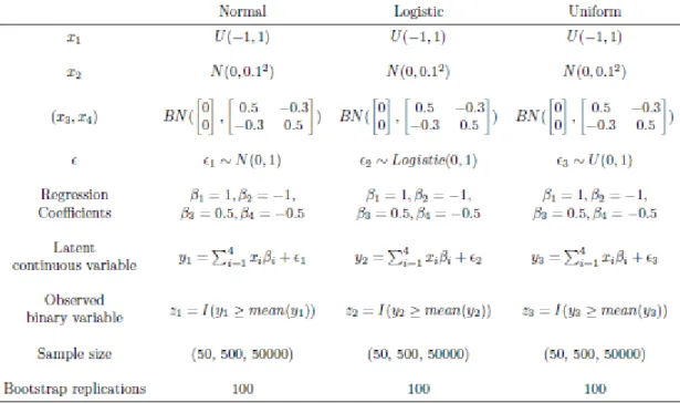
We generate a population of total sample size n = 1,000,000. The simulation process is:
Step 1: generate 4 covariates, simulated as follows: 𝑥1 ~ 𝑈
(
−1,1)
, 𝑥2 ~ 𝑁(0, 0.12), and 𝑥3 , 𝑥4 from abivariate normal distribution with means zeros and covariance matrix
(
0.5 −0.3 −0.3 0.5)
.
Step 2: generate error variables from each of the following three standard error distributions: 𝜀1~𝑁
(
0,1)
, 𝜀2~𝐿𝑜𝑔𝑖𝑠𝑡𝑖𝑐(0,1), and 𝜀3~ 𝑈(0,1).Step 3: calculate three latent (dependent) variables that correspond to the three error distributions and use the fixed parameter values 𝛽0= 0, 𝛽1 = 1, 𝛽2= −1, 𝛽3= 0.5, 𝛽4 = −0.5:
𝑌1 = 𝛽0+ 𝛽1𝑥1+ 𝛽2𝑥2+ 𝛽3𝑥3+ 𝛽4𝑥4+ 𝜀1 (15)
𝑌2 = 𝛽0+ 𝛽1𝑥1+ 𝛽2𝑥2+ 𝛽3𝑥3+ 𝛽4𝑥4+ 𝜀2
𝑌3 = 𝛽0+ 𝛽1𝑥1+ 𝛽2𝑥2+ 𝛽3𝑥3+ 𝛽4𝑥4+ 𝜀3
Step 4: calculate the observed binary variable for each latent dependent variable by using the mean as the cut-off threshold. Using the indicator functionΙ(. ), which results in a dummy variable with value 1 if the condition is true and 0 if it is false, we calculate 𝑍1 =Ι
(
𝑌1 ≥ 𝑚𝑒𝑎𝑛(
𝑌1)), 𝑍2 = Ι(
𝑌2 ≥ 𝑚𝑒𝑎𝑛(
𝑌2)),𝑍3 = Ι
(
𝑌3 ≥ 𝑚𝑒𝑎𝑛(
𝑌3))
.
From this population data, we sample three datasets with different sample sizes (n = 50, n = 500, n = 50,000). Figure 2 summarizes the study design.
4.1.2
Analyses and Results
Based on the above design, our study was a 3 x 3 x 3 factorial design: three sample sizes (n = 50, n = 500, n = 50,000), three standard error distributions (normal, logistic, and uniform), and three estimated models (Probit, Logit, and LPM). In addition, to evaluate sampling variability, we simulated 100 replications in each cell (for each of the 27 combinations of sample size, error distribution, and estimated model).
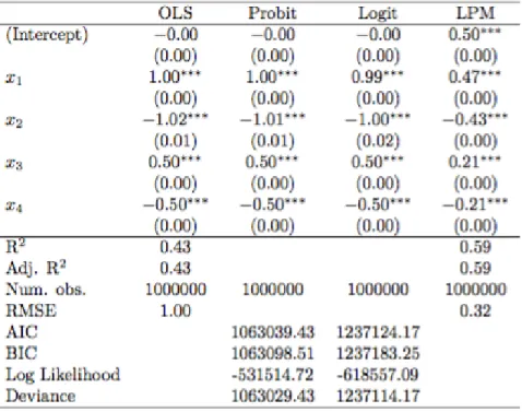
Before performing the analyses, we estimated all the models using the population data. Figure 3 shows the results. The first column gives the output for the estimated model with the continuous dependent variable 𝑌1, which serves as a baseline model. The other columns in Figure 3 show the results from probit,
logit, and linear probability models with the dependent variables 𝑍1, 𝑍2, and 𝑍3
,
respectively. Weestimated each model using the data generated from the appropriate distribution—the ideal scenario (i.e., we estimated a logistic model using the data simulated from a logistic error distribution, etc.).
Figure 3. Estimated Models on Total Data (“Population”)3
From Figure 3, we see that the estimates from the LPM were proportional to and directionally consistent with the estimates from the baseline (continuous 𝑌1) model.
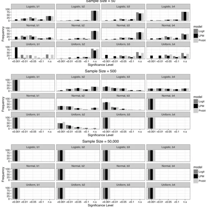
We first examined inference: we evaluated the coefficient significance levels in each of the 27 combinations. Figure 4 describes the results for each of the three sample sizes. The x-axis represents common significance levels, and the y-axis is the frequency (or percentage) out of 100 replications. Rows represent different error distributions and columns represent the regression coefficients (𝛽
̂
1, 𝛽̂
2, 𝛽̂
3, 𝛽̂
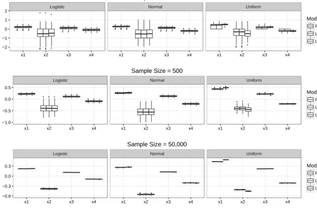
4). We can observe that the coefficient significance levels were similar for the three models across all the coefficients and for the given three sample sizes. Although we can observe a small discrepancy for the uniform errors for n = 50, the bars for the non-significant (n.s) level were very similar. The violation of distributional assumptions matters for small samples such as n = 50 but, with large samples, these differences disappear. Figure 5 shows the marginal effects for the estimated models for each sample size. The three subplots in each row are for different error distributions. We plotted the estimated marginal effects for the 100 replications as a boxplot to show their distribution. We can observe that the distribution of marginal effects for each of the three models and for all the coefficients were nearly identical. Since 𝑥2 had very small3 Dependent variables: Y
variance, 𝛽
̂
2 exhibited larger variance compared to other coefficients. With large samples, marginal effects were very precise and also similar across all three models.Figure 4. Comparing the Three Models in Terms of Frequency of Coefficient Significance by Sample Size; Results Based on 100 Replications for Each of the Sample Data Sets4
4 We calculated the significance values using Robust standard errors, which we computed using the HC1 formulation in R package
Figure 5. Comparing the Three Models in Terms of the Marginal Effects Distribution Across 100 Replications for Each Sample Size
4.2
Prediction and Selection Bias
4.2.1
Simulation Design
We based the simulation for the prediction analyses on the models we describe in Section 2.1. We simulated a dataset of size n = 1,000,000 and set initial parameters to the following values: 𝛾0 = −0.5, 𝛾1 = 0.5, 𝛾2= −0.5, 𝛾3 = 1.5, 𝛾4= −1, 𝛽0 = 0.5, 𝛽1= −1.5, 𝛽2= 0.5, 𝛽3 = 1
Step 1: generate (𝜔, 𝜀) from a bivariate normal distribution with means 0 and covariance
(
0.5 −0.4 −0.4 0.5)
.
Step 2: generate 𝑥1~ 𝑈
(
0,1)
, 𝑥2~ 𝑁(0,1), and 𝑥3, 𝑥4 from a bivariate normal distribution with means 0.5and covariance
(
0.5 0.3 0.3 0.5)
.Step 3: selection model: compute s* using the formula 𝑆∗ = 𝛾0+ 𝛾1𝑥1+ 𝛾2𝑥2+ 𝛾3𝑥3+ 𝛾4𝑥4+ 𝜔 and 𝑆 =
Ι(𝑆∗≥ 𝑚𝑒𝑎𝑛(𝑆∗)).
Step 4: outcome model: for S = 1, compute Y using the formula: 𝑌 = 𝛽0+ 𝛽1𝑥1+ 𝛽2𝑥2+ 𝛽3𝑥3+ 𝜀.
We used the data from the above design to estimate the outcome model under selection bias.
4.2.2
Analyses and Results
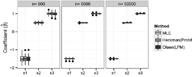
Similar to the inference and estimation case, we sampled three datasets with sizes n = 500, n = 5000, and n = 50,000. Again, we simulated 100 replications for each combination of sample size and for each model. Figure 6 plots the results in terms of the outcome model coefficients’ distribution.
In addition to comparing the outcome model coefficients, which are of interest in selection bias scenarios, we also compared the predictions of the probit, logit and linear probability models on a holdout set. Such predictions are of interest in predictive studies. Figure A1 shows the results. We can see that the
● ● ● ● ● ● ● ● ● ● ● ● ● ● ● ● ● ● ● ● ● ● ● ● ● ● ● ● ● ● ● ● ● ● ● ● ● ● ● ● ● ●●● ● ● ●
Logistic Normal Uniform
−2 −1 0 1 2 x1 x2 x3 x4 x1 x2 x3 x4 x1 x2 x3 x4 M a rg in a l E ff e c t (M E ^) Model Probit Logit LPM Sample Size = 50 ● ● ● ● ● ● ● ● ● ● ● ● ● ● ● ● ● ● ● ● ● ● ●
Logistic Normal Uniform
−1.0 −0.5 0.0 0.5 x1 x2 x3 x4 x1 x2 x3 x4 x1 x2 x3 x4 M a rg in a l E ff e c t (M E ^) Model Probit Logit LPM Sample Size = 500 ● ● ● ● ● ● ● ● ● ● ● ● ● ● ● ● ● ● ● ● ● ● ● ● ● ● ● ● ● ● ● ● ●
Logistic Normal Uniform
−0.6 −0.3 0.0 0.3 x1 x2 x3 x4 x1 x2 x3 x4 x1 x2 x3 x4 M a rg in a l E ff e c t (M E ^) Model Probit Logit LPM Sample Size = 50,000
prediction distributions from all three models were identical except for the LPM’s unbounded predictions. This finding also corroborates the selection bias results.
Figure 6. Comparing the Coefficient Distribution in a 2SLS Outcome Model after Correcting for Selection Bias with Three Methods; Results by Sample Size based on 100 Bootstrap Replications
5
An Application to Online Auctions
Online auction websites produce large amounts of data that one can use to provide services to buyers and sellers, for market research, and for product development. Therefore, academic research that uses online auction data has thrived in various disciplines, including information systems, marketing, computer science, statistics, and economics. Early studies looked at determinants of auction price to identify and quantify factors that affect an auction’s final price (Lucking-Reiley, Bryan, Prasad, & Reeves, 2007); other studies have looked at price dynamics; the development of models for forecasting auction prices and for studying bidder and seller relationships; and more (see Jank & Shmueli, 2010).
To illustrate and evaluate the use of LPMs in the context of a real dataset, we used a large sample (n = 300,384) of eBay (www.ebay.com) auctions for digital cameras that transacted between August 2007 and January 2008. Lin et al. (2013) used the same dataset. We sought to: 1) quantify the relationship between auction price (the outcome) and four covariates of interest: auction duration, minimum bid5, and whether
the seller set a reserve price6 or not (the covariates in the model that Lin et al. (2013) used); and 2) predict
the price of new auctions given these four predictors.
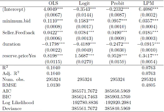
Figure 7 provides the summary statistics for the variables, and one can see that they are severely skewed with possibly extreme outliers. To be able to evaluate the LPM against benchmarks, we dichotomized the price variable using a median split, so that prices above the median were set to 𝑍 = 1 and otherwise to 𝑍 = 0. We estimated all the four models we describe in Section 5.1. We used a holdout sample of size n = 5,000 to evaluate the predictions from the above models. First, we compared the LPM coefficients and their significance with probit, logit, and OLS regression using the continuous price after a log-transformation (ln(Price)) to account for skewness in price7 (Figure A28).
5 The seller sets the minimum bid and the auction duration before the start of the auction.
6 A reserve price is a secret threshold set by the seller. The auction will not transact unless the price exceeds this threshold. 7 Ideally, we would use a Box-Cox transformation with parameter for the price variable to achieve normality. However, using
a log transformation enables meaningful coefficient interpretation.
Figure 7. Summary Statistics for the eBay Auction Variables
Figure 8 describes the results. Both logit and probit models suffered quasi-separation issues (discussed in previous sections) due to severe skewness in the covariates. Figure A6 provides the residual diagnostic plots for the logit model. One can see from the plot that the data contained serious outliers that caused both the logit and probit models to suffer from quasi-separation warnings, while the LPM had no such estimation problems. To avoid this problem, for the inference purpose, we log transformed the three continuous covariates. Column 1 presents the results from OLS regression on the continuous price variables, which we can use as a benchmark. The remaining three models (logit, probit and LPM) used binary price as the dependent variable.
We can immediately see that estimates for both probit and logit look different, which contrasts with what we observed in the simulation results. This issue is not specific to the current data and is not rare in practice. As we mention earlier, we need to scale the logit coefficients by 1.7 to obtain the probit coefficients. Similarly, the coefficients from the LPM are proportional to the true coefficients9. One can see
that the direction and the significance results across all the models are identical. We compared coefficient significance and marginal analysis as in the simulation. The results (Figure A3) are consistent with both theory and what we observed in the simulation study.
Figure 8. Estimated OLS and LPM Models for Price of Online Auctions
In terms of predictive power, we compared the out-of-sample predictions and classifications from the LPM to those from a logit and probit models for the holdout sample. While variable transformations are good for coefficient estimation (explanatory modeling), sometimes modeling the raw data leads to higher predictive performance. Therefore, we compared predictions from models with unstandardized covariates (Figure 9) to predictions from models without log transformed covariates (Figure A4 in Appendix). Figure 9 shows good class separation by all models, while Figure A4 shows less class separation. And, indeed, we see that the predictive power of the models that used binary price on raw data (or covariates) was much better than the models using binary price on log transformed data (or covariates). Note that some LPM predictions exceeded the unit interval.
In the boxplots, the LPM predictions appear to have slightly lower variance within each class but closer class medians. We also note that the area under the curve (AUC) values for the three models are identical. Thus, for a predictive purpose, if one seeks class separation alone, then the LPM is as good as the logit and probit models. However, since the predicted probabilities exceeded the unit interval, LPMs are not a good choice if one seeks the predicted probabilities themselves.
Figure 9. Predictions (Left) and ROC Curves (Right) for the Holdout Price Data for Logit, Probit, and Linear Probability Models (Unstandardized Covariates)
6
Summary and Conclusions
The results from both the simulation study and eBay analysis indicate that LPMs perform similar to logistic and probit models in terms of coefficient significance, effect size (marginal effect), classification, and ranking. LPM coefficients have the added advantage of easier interpretation, but LPMs are inferior to logit and probit models if predicted probabilities are of interest.
Revisiting our literature survey, we note that, in almost all of the studies, the authors could have considered using a LPM in place of the logit or probit model they used. Specifically, in all of the selection model cases except for the paper that used Tobit due to truncation, the authors could have used a LPM. Using a LPM in place of a probit model in the first stage of 2SLS is simpler than using a probit model because it does not require computing the Mills ratio. For papers that performed classification, LPM would have been a reasonable model in place of the logistic regression: in Kohli and Devaraj (2003) and in Bardhan, Oh, Zheng, and Kirksey (2015). In contrast, Hui et al. (2007) report both predicted classes and probabilities, and, therefore, a LPM would not have been a good choice. Lastly, for the inference and estimation studies, in all cases where the authors used the binary outcome model for obtaining statistical significance, coefficient sign, or marginal effects, a LPM would have again been a reasonable alternative. For marginal effects, LPMs are especially useful because they do not require extra calculations (as is the case in linear regression for a continuous outcome). For example, Bloom, Garicano, Sadun, and Van Reenen (2014) compared the effect size of different independent variables on several outcomes of interest (some of which were continuous and some binary). They fitted OLS to the numerical outcome models and probit to the binary outcome models. For interpreting the effects, they relied on the OLS
coefficients directly but had to perform and report marginal effects for the probit models. Had they used a LPM, they would have simplified the exposition and been able to straightforwardly compare and interpret the different models of interest.
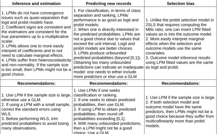
Our results illustrate that LPMs have advantages and disadvantages when compared to GLMs for a binary outcome variable. We see that whether one should use a LPM closely depends on one’s analysis goal. For inference and parameter estimation, LPMs are mainly useful due to their simplicity and ease of interpretation. For generating predicted or fitted values from selection models or for classification, LPMs are as good as logit and probit models in terms of class separation and ranking. LMPs are inappropriate only when the predicted probabilities themselves are the quantities of interest. We also show that LPMs perform equally to other selection bias models. Finally, in terms of inference, LPMs provide a superior alternative for data where the logit and probit models do not converge or issue quasi-separation warnings (e.g., our eBay example). We summarize the advantages and weaknesses of LPM in Table 2.
Table 2. Summary of the LPM Results: Advantages and Shortcomings of LPM for Different Study Goals Inference and estimation Predicting new records Selection bias
1. LPMs do not have convergence issues such as quasi-separation that logit and probit models have.
2. Coefficient signs are consistent and the estimators are consistent for the true parameters up to a multiplicative scalar.
3. LPMs allows one to more easily interpret of coefficients and to not need to calculate marginal effects. 4. LPMs suffer from heteroscedasticity and non-normality. If the sample size is too small, then LPMs might not be a good choice.
1. For classification, in terms of class separation and ranking, LPMs’ performance is as good as logit and probit models.
2. When one is directly interested in the predicted probabilities, LPMs are not a good choice due to values that exceed the unit interval. Logit and probit models are better choices. 3. LPMs produce unbounded predicted probabilities (beyond [0,1]). Obtaining too many unbounded predictions can indicate an inadequate model: one needs to either include more predictors or else use a GLM
1. Unlike the probit selection model in 2SLS that requires computing the Mills ratio, one can insert LPM fitted values as-is into the outcome model. 2. More easily interpret marginal effects when the selection and outcome models use the same covariates.
3. Outcome model inference results using LPM fitted values are the same as logit and probit.
Recommendations: Recommendations: Recommendations:
1. Use LPM if the sample size is large, otherwise use a GLM.
2. If using a LPM with a small sample, correct the standard errors using WLS.
3. Before performing WLS, trim predicted probabilities to avoid losing many observations.
1. Use LPMs if one seeks classification or ranking.
2. If one seeks to obtain predicted probabilities, then use GLM. 3. If using LPM to obtain predicted probabilities, then round off probabilities exceeding [0,1].
4. With many unbounded predictions, then a LPM might not be a good choice. Use a GLM.
1. Use LPM if the sample size is large. 2. If both selection model and
outcome model have the same predictors, then LPMs might not be a good choice because they suffer from multicollinearity more than probit models.
As Table 2 shows, and consistent with the literature, the LPM estimators are consistent for the true parameters up to a multiplicative scalar. One can calculate the scalar if one has a reasonable estimate of 𝜎𝑦 .However, we
reiterate that one needs the standard deviation only to retrieve the underlying true (OLS) coefficient, which is often not a researcher’s primary interest. When really needed, however, one could obtain an estimate of the standard deviation based on subject knowledge (similar to Bayesian priors) or by using previous studies that use a continuous outcome variable. One could also take a small sample of the continuous outcome variable when it is expensive to collect it for the entire study sample. In addition to the coefficient proportionality property, the coefficient significance and direction are consistent with logit and probit models.
Our simulation results on coefficient significance agree with the results that Hellevik (2009) reports. However, our study differs from Hellevik (2009) in terms of objectives and contributions. They are similar only to Hellevik’s (2009) results that compared the significance probabilities of linear probability and logit models. While Hellevik (2009) focuses only on the coefficients’ statistical significance, we also examine prediction and selection bias issues. Our simulation settings are more comprehensive. We used four covariates both in the simulation and in a real dataset (eBay) with different types of variable distributions, while Hellevik (2009) used only two covariates (one continuous, one binary). We also used varying sample sizes (n = 50, 500, and 50000) to observe the consistent behavior of the estimators. Lastly, we also included the probit model in our comparisons, whereas Helevik (2009) only compared LPMs with logit
models. Hence, our approach and results provide a more comprehensive picture about LPMs’ performance compared to logit and probit models. As we move into the realm of big data, we need to consider analyses’ computational costs. With the advances in computing power, logit and probit models estimation is typically sufficiently fast despite the iterative nature of the estimation algorithm. LPMs produce results in a single iteration and are computationally cheaper. Hence, when one seeks to obtain real time predictions or where one needs to update the model frequently (e.g., every minute), LPMs might be advantageous. Table A2 describes the computation times for our simulation study in Section 4.1 (model with four predictors).
One question for future research involves using LPMs with multi-category outcome variables. For example, in propensity score matching, research has shown that logit and probit selection models have negligible differences with a binary outcome but that they do have different strengths in the multi-class case (Caliendo, 2006, p.73). Second, our simulation study was limited to the manipulated variables we chose. One could extend our study by expanding the simulation models to a large number of predictors and non-linear relationships such as interaction terms. Our initial findings from exploring nonlinear models indicate that the results remain unchanged as long as no severe multicollinearity affects LPM estimation. Finally, another direction of interest is LPMs’ performance compared to logit or probit models in the case of highly unbalanced data, where the number of 1s is very small or very large.
Acknowledgments
We thank Ravi Bapna and Nishtha Langer for emphasizing the importance of studying LPMs for selection bias and Wolfgang Jank for sharing the eBay data. We are grateful to the AE and the three reviewers for their helpful comments and suggestions that helped improve this paper. This research was partially funded by grant 105-2410-H-007-034-MY3 from the Ministry of Science and Technology in Taiwan.
References
Abbasi, A., Sarker, S., & Chiang, R. H. (2016). Big data research in information systems: Toward an inclusive research agenda. Journal of the Association for Information Systems, 17(2), i-xxxii.
Adjerid, I., Acquisti, A., Telang, R., Padman, R., & Adler-Milstein, J. (2015). The impact of privacy regulation and technology incentives: The case of health information exchanges. Management Science, 62(4), 1042-1063.
Agarwal, R., & Dhar, V. (2014). Big data, data science, and analytics: The opportunity and challenge for IS research. Information Systems Research, 25(3), 443-448.
Aggarwal, R., Gopal, R., Gupta, A., & Singh, H. (2012). Putting money where the mouths are: The relation between venture financing and electronic word-of-mouth. Information Systems Research, 23(3), 976-992.
Aggarwal, R., Kryscynski, D., Midha, V., & Singh, H. (2015). Early to adopt and early to discontinue: The impact of self-perceived and actual IT knowledge on technology use behaviors of end users.
Information Systems Research, 26(1), 127-144.
Aggarwal, R., & Singh, H. (2013). Differential influence of blogs across different stages of decision making: The case of venture capitalists. MIS Quarterly, 37(4), 1093-1112.
Aldrich, J. H., & Nelson, F. D. (1984). Linear probability, logit, and probit models (vol. 45). Thousand Oaks, CA: Sage.
Anderson, G. J. (1987). Prediction tests in limited dependent variable models. Journal of Econometrics, 34(1), 253-261.
Angrist, J. D., & Pischke, J. S. (2008). Mostly harmless econometrics: An empiricist's companion.
Princeton, NJ:Princeton University Press.
Angrist, J. D., & Pischke, J. S. (2012). Probit better than LPM? MostlyHarmlessEconometrics. Retrieved from http://www.mostlyharmlesseconometrics.com/2012/07/probit-better-than-lpm/
Aral, S., Brynjolfsson, E., & Wu, L. (2012). Three-way complementarities: Performance pay, human resource analytics, and information technology. Management Science, 58(5), 913-931.
Asvanund, A., Clay, K., Krishnan, R., & Smith, M. D. (2004). An empirical analysis of network externalities in peer-to-peer music-sharing networks. Information Systems Research, 15(2), 155-174.
Banker, R. D., Hu, N., Pavlou, P. A., & Luftman, J. (2011). CIO reporting structure, strategic positioning, and firm performance. MIS Quarterly, 35(2), 487-504.
Bapna, R., Goes, P., Wei, K. K., & Zhang, Z. (2011). A finite mixture logit model to segment and predict electronic payments system adoption. Information Systems Research, 22(1), 118-133.
Bardhan, I., Oh, J. H., Zheng, Z., & Kirksey, K. (2015). Predictive analytics for readmission of patients with congestive heart failure. Information Systems Research, 26(1), 19-39.
Benaroch, M., Lichtenstein, Y., & Robinson, K. (2006). Real options in information technology risk management: An empirical validation of risk-option relationships. MIS Quarterly, 30(4), 827-864. Betts, J. R., & Fairlie, R. W. (2001). Explaining ethnic, racial, and immigrant differences in private school
attendance. Journal of Urban Economics, 50(1), 26-51.
Bloom, N., Garicano, L., Sadun, R., & Van Reenen, J. (2014). The distinct effects of information technology and communication technology on firm organization. Management Science, 60(12), 2859-2885.
Brillinger, D. R. (2012). A generalized linear model with “Gaussian” regressor variables. In D. R. Brillinger (Ed.), Selected works of David Brillinger (pp. 589-606). Berlin: Springer.
Burtch, G., Ghose, A., & Wattal, S. (2016). Secret admirers: An empirical examination of information hiding and contribution dynamics in online crowdfunding. Information Systems Research, 27(3), 478-496.
Caliendo, M., Clement, M., Papies, D., & Scheel-Kopeinig, S. (2012). The cost impact of spam filters: Measuring the effect of information system technologies in organizations. Information Systems Research, 23(3), 1068-1080.
Caudill, S. B. (1987). Dichotomous choice models and dummy variables. The Statistician, 36, 381-383. Caliendo, M. (2006). Microeconometric evaluation of labour market policies (vol. 568). Berlin: Springer. Ceccagnoli, M., Forman, C., Huang, P., & Wu, D. J. (2011). Co-creation of value in a platform ecosystem:
The case of enterprise software. MIS Quarterly, 36(1), 263-290.
Chan, J., & Ghose, A. (2013). Internet’s dirty secret: Assessing the impact of online intermediaries on HIV transmission. MIS Quarterly, 38(4), 955-976.
Chang, Y. B., & Gurbaxani, V. (2012). Information technology outsourcing, knowledge transfer, and firm productivity: An empirical analysis. MIS Quarterly, 36(4), 1043-1053.
Chau, P. Y., & Tam, K. Y. (1997). Factors affecting the adoption of open systems: An exploratory study.
MIS Quarterly, 21(1), 1-24.
Chen, P. Y., & Forman, C. (2006). Can vendors influence switching costs and compatibility in an environment with open standards? MIS Quarterly, 30(SI), 541-562.
Chen, P. Y., & Hitt, L. M. (2002). Measuring switching costs and the determinants of customer retention in Internet-enabled businesses: A study of the online brokerage industry. Information Systems Research, 13(3), 255-274.
Chen, Y., & Bharadwaj, A. (2009). An empirical analysis of contract structures in IT outsourcing.
Information Systems Research, 20(4), 484-506.
De, P., Hu, Y., & Rahman, M. S. (2013). Product-oriented Web technologies and product returns: An exploratory study. Information Systems Research, 24(4), 998-1010.
Duan, N., & Li, K. C. (1991). A bias bound for least squares linear regression. Statistica Sinica, 1(1991), 127-136.
Duda, R. O., Hart, P. E., & Stork, D. G. (2012). Pattern classification. New York: John Wiley & Sons. Fairlie, R. W., & Sundstrom, W. A. (1999). The emergence, persistence, and recent widening of the racial
unemployment gap. Industrial & Labor Relations Review, 52(2), 252-270.
Fang, Z., Gu, B., Luo, X., & Xu, Y. (2015). Contemporaneous and delayed sales impact of location-based mobile promotions. Information Systems Research, 26(3), 552-564.
Fisher, R. A. (1936). The use of multiple measurements in taxonomic problems. Annals of Eugenics, 7(2), 179-188.
Fitoussi, D., & Gurbaxani, V. (2012). IT outsourcing contracts and performance measurement. Information Systems Research, 23(1), 129-143.
Forman, C., Ghose, A., & Wiesenfeld, B. (2008). Examining the relationship between reviews and sales: The role of reviewer identity disclosure in electronic markets. Information Systems Research, 19(3), 291-313.
Forman, C., Ghose, A., & Goldfarb, A. (2009). Competition between local and electronic markets: How the benefit of buying online depends on where you live. Management Science, 55(1), 47-57.
Friedman, J., Hastie, T., & Tibshirani, R. (2009). The elements of statistical learning (2nd ed.). Berlin:
Springer.
Gefen, D., & Carmel, E. (2008). Is the world really flat? A look at offshoring at an online programming marketplace. MIS Quarterly, 32(2), 367-384.
Gao, G., Greenwood, B. N., Agarwal, R., & Jeffrey, S. (2015). Vocal minority and silent majority: How do online ratings reflect population perceptions of quality? MIS Quarterly, 39(3), 565-589.
Godinho de Matos, M., Ferreira, P., & Krackhardt, D. (2014). Peer influence in the diffusion of the iPhone 3G over a large social network. Management Information Systems Quarterly, 38(4), 1103-1133.
Goes, P. B., Lin, M., & Au Yeung, C. M. (2014). “Popularity effect” in user-generated content: Evidence from online product reviews. Information Systems Research, 25(2), 222-238.
Goh, K. Y., Heng, C. S., & Lin, Z. (2013). Social media brand community and consumer behavior: Quantifying the relative impact of user-and marketer-generated content. Information Systems Research, 24(1), 88-107.
Goldberger, A. S. (1964). Econometric theory. New York: Wiley.
Gopal, A., & Koka, B. R. (2012). The asymmetric benefits of relational flexibility: evidence from software development outsourcing. MIS Quarterly, 36(2), 553-576.
Gopal, A., & Sivaramakrishnan, K. (2008). On vendor preferences for contract types in offshore software projects: The case of fixed price vs. time and materials contracts. Information Systems Research, 19(2), 202-220.
Gordon, D. V., Lin, Z., Osberg, L., & Phipps, S. (1994). Predicting probabilities: Inherent and sampling variability in the estimation of discrete-choice models. Oxford Bulletin of Economics and Statistics, 56(1), 13-31.
Gordon, L. A., Loeb, M. P., & Sohail, T. (2010). Mark