NBER WORKING PAPER SERIES
VARIABLE RARE DISASTERS:
AN EXACTLY SOLVED FRAMEWORK FOR TEN PUZZLES IN MACRO-FINANCE
Xavier Gabaix
Working Paper 13724
http://www.nber.org/papers/w13724
NATIONAL BUREAU OF ECONOMIC RESEARCH
1050 Massachusetts Avenue
Cambridge, MA 02138
January 2008
For helpful conversations and comments, I thank Robert Barro, David Chapman, Alex Edmans, Emmanuel
Farhi, Francois Gourio, Sydney Ludvigson, Anthony Lynch, Thomas Philippon, José Scheinkman,
Stijn Van Nieuwerburgh, Adrien Verdelan, Stanley Zin, and seminar participants at Duke, Harvard,
Minnesota Workshop in Macro Theory, MIT, NBER, Paris School of Economics, Princeton, Texas
Finance Festival, UCLA, and Washington University at Saint Louis. I thank the NSF for support. The
views expressed herein are those of the author(s) and do not necessarily reflect the views of the National
Bureau of Economic Research.
NBER working papers are circulated for discussion and comment purposes. They have not been
peer-reviewed or been subject to the review by the NBER Board of Directors that accompanies official
NBER publications.
© 2008 by Xavier Gabaix. All rights reserved. Short sections of text, not to exceed two paragraphs,
may be quoted without explicit permission provided that full credit, including © notice, is given to
the source.
Variable Rare Disasters: An Exactly Solved Framework for Ten Puzzles in Macro-Finance
Xavier Gabaix
NBER Working Paper No. 13724
January 200
8
JEL No. E43,E44,G12
ABSTRACT
This paper incorporates a time-varying intensity of disasters in the Rietz-Barro hypothesis that risk
premia result from the possibility of rare, large disasters. During a disaster, an asset's fundamental
value falls by a time-varying amount. This in turn generates time-varying risk premia and thus volatile
asset prices and return predictability. Using the recent technique of linearity-generating processes (Gabaix
2007), the model is tractable, and all prices are exactly solved in closed form. In the "variable rare
disasters" framework, the following empirical regularities can be understood qualitatively: (i) equity
premium puzzle (ii) risk-free rate-puzzle (iii) excess volatility puzzle (iv) predictability of aggregate
stock market returns with price-dividend ratios (v) value premium (vi) often greater explanatory power
of characteristics than covariances for asset returns (vii) upward sloping nominal yield curve (viiii)
a steep yield curve predicts high bond excess returns and a fall in long term rates (ix) corporate bond
spread puzzle (x) high price of deep out-of-the-money puts. I also provide a calibration in which those
puzzles can be understood quantitatively as well. The fear of disaster can be interpreted literally, or
can be viewed as a tractable way to model time-varying risk-aversion or investor sentiment.
Xavier Gabaix
New York University
Finance Department
Stern School of Business
44 West 4th Street, 9th floor
New York, NY 10012
and NBER
1
Introduction
Lately, there has been a revival of a hypothesis proposed by Rietz (1988), that the possibility of rare disasters (such as economic depressions or wars) is a major determinant of asset risk premia. Indeed, Barro (2006) has shown that, internationally, disasters have been sufficiently frequent and large to make the Rietz’ proposal viable, and account for the high risk premium on equities.
The Rietz-Barro hypothesis is almost always formulated with constant intensity of disasters. This is useful to think about long run average, but cannot account for some key features of asset markets, such as volatile price-dividend ratios for stocks, volatile bond risk premia, and return predictability1 In the present paper, I formulate a variable-intensity version of the rare disasters hypothesis, and investigate the impact of time-varying disaster intensity on the prices of stocks and bonds, and the predictability of their returns. A later companion paper (Farhi and Gabaix 2007) studies exchange rates.
I lay out and analyze the model, which I dub the “variable rare disasters” model. I show that many asset puzzles can be qualitatively understood using this model. I then ask whether a parsimonious calibration can allow to understand them quantitatively, andfind that, provided one assumes a variable enough sensitivity of real and nominal variables to disasters (something I will argue below is plausible), those puzzles can be understood quantitatively as well.
I conclude that the rare disaster hypothesis, augmented by a time-varying intensity of disaster as proposed in this paper, is a workable additional paradigm for macro-finance. Indeed, within the class of rational, representative-agents frameworks, it may be viewed as a third workable paradigm, along the external habit model of Campbell-Cochrane (1999), and the long run risk model of Bansal and Yaron (2004). I contrast those models below.
In the present paper, the value loss suffered by assets in a disaster varies both along the cross-section and over time. Hence, assets have time-varying risk premia, which generates volatile prices. For instance, stock prices are high when stocks bear little risk, i.e. would suffer only a small value loss in a disaster. This perceived riskiness mean-reverts, which leads to a mean-reversion of the price-dividend ratio of stocks. Hence stocks exhibit “excess volatility” caused by their stochastic riskiness and risk premia.
The proposed framework allows for a very tractable model of stock and bonds, in which all prices are in closed forms. It offers a framework in which the following patterns are not puzzles, but they emerge naturally when the present model has two shocks, one real, for stocks, and one nominal, for bonds.
A. Stock market: Puzzles about the aggregates
1. Equity premium puzzle. 1
The only exception I am aware of is Longstaffand Piazzesi (2004). They consider an economy with constant intensity of disasters, but in which stock dividends are a variable, mean-reverting share of consumption. Theyfind a high equity premium, and highly volatile stock returns. Finally, Weitzman (2007) provides a Bayesian view that the main risk is model uncertainty, as the true volatility of consumption may be much higher than the sample volatility. Unlike the present work, those papers do not consider bonds, nor study return predictability.
2. Risk-free rate puzzle.2
3. Excess volatility puzzle: Stock prices are more volatile than warranted by a model with a constant discount rate.
4. Aggregate return predictability: Future aggregate stock market returns are partly predicted by Price/Earnings and Price/Dividend ratios, and the Consumption/Aggregate wealth ratio.
B. Stock market: Puzzles about the cross-section of stocks
5. Value/Growth puzzle: Stocks with a high (resp. low) P/D ratio have lower (resp. high) future returns, even controlling for their covariance the aggregate stock market.
6. Characteristics vs Covariances puzzles: Stock characteristics (e.g. the P/D ratio) often predict future returns as well or better than covariances with risk factors.
C. Nominal bond puzzles: Yield curve
7. The yield curve slopes up on average. The premium of long-term yields over short-term yields is too high to be explained by a traditional RBC model. This is the mirror image of the equity premium puzzle for bonds.
8. Fama-Bliss, Campbell-Shiller, Cochrane-Piazzesi facts: A high slope of the yield curve predicts excess high positive returns on long term bonds, and that long term interest rates will fall.
D. Nominal bond puzzles: Credit spreads
9. Corporate bond spreads are higher than seemingly warranted by historical default rates.
E. Options
10. High price of deep of out-of-the-money puts.
To understand the economics of the model,first consider bonds. Consistent with the empirical evidence (Barro 2006), in the model, a disaster leads to a temporary jump in inflation. This has a greater detrimental impact on long-term bonds, and so they command a high risk premium relative to short-term bonds. This explains the upward slope of the nominal yield curve. Next, suppose that expected jump in inflation itself varies. Then the slope of the yield curve will vary, and will predict excess bond returns. A high slope will mean-revert, hence predicts a fall in long rate, and high returns on long term bonds. This mechanism accounts for many stylized facts on bonds.
2For this and the above puzzle, the paper simply imports from Rietz (1988), Longstaff and Piazzesi (2004) and Barro (2006).
The same mechanism is at work for stocks. Suppose that a disaster reduces the fundamental value of a stock by a time-varying amount. This yields a time-varying risk premium which generates a time-varying price-dividend ratio, and “excess volatility” of stock prices. It also makes stock returns predictable via measures such as the dividend-price ratio. When agents perceive the intensity of disasters as low, the price-dividend ratios are high, and future returns are low.
Using this logic in the cross-section, the model offers a way to think about value and growth stocks: stocks with low price-dividend ratios (value stock) have high subsequent returns. I hasten to say that this interpretation of value stocks is more speculative than the rest of the paper. To assess it, one would like to know how badly value versus growth stocks fared during historical disasters, across many countries. It is at least conceivable that value firms were “distressed” firms that did particularly badly during disasters.
After laying out the framework, I ask if some parameters can rationalize the fairly large volatility of asset prices, and values that can. The average values are essentially taken from Barro (2006)’s analysis of many countries, a project being expanded in Barro and Ursua (2007). The volatilities of expectation about disaster sizes are very hard to measure directly. However, the numbers calibrated in this paper generates a steady state dispersion of anticipations that is almost certainly lower than the dispersion of realized values. By that criterion, the calibrated values in the model appear reasonable. Still, whether there are is ultimately an empirical question. However, it is beyond the scope and spirit of this paper to provide new historical results. This paper is essentially only theoretical — it lays out the framework of variable rare disaster, solves it, and provides a calibration. The calibration that gives consistent results for stocks, bonds and options.
The model also studies disaster-related assets, such as corporate bonds, and options. If high-quality corporate bonds default mostly during disasters, then they should command a high premium, that cannot be accounted for by their behavior during normal times. Likewise, I derive options prices. The model generates a “volatility smirk”, i.e. a high put price (hence implied volatility) for deep out-of-the-money puts. The model’s calibration seems quite close to empirical values. I also suggest how options prices might reveal the underlying disaster risk premia.
The model is presented as fully rational, but it could be interpreted as a behavioral model. The changing beliefs about the intensity of possible disasters are very close to what the behavioral literature calls “animal spirits,” and the recent rational literature calls “perception of distant risks”, or “time-varying risk aversion”. The model’s structure gives a consistent way to think about the impact of changing “sentiment” on prices, in the time-series and the cross-section.3
Throughout the paper, I use the class of “linearity-generating” processes (Gabaix 2007). That class keeps all expressions in closed form. The entire paper could be rewritten with other processes (e.g. affi ne-yield models) albeit with considerably more complicated algebra, and the need to resort to numerical
3
solutions. I suspect that the economics would be similar (the linearity-generating class and the affine class give the same expression to afirst order approximation). Hence, there is little of economic consequence in the use of linearity-generating processes, and they should be viewed as simply an analytical convenience.
Relation to the literature This project of a single framework for stocks, bonds and exchange rates is motivated by Cochrane (1999), who emphasized the similarities in puzzles about those three assets. These concern chiefly the patterns of “excess volatility” and return predictability. These similarities suggest that the same microfoundations may have the potential to explain the empirical regularities in all three asset markets. Specifically, across all three asset markets, a simple “return-chasing” strategy appears to deliver superior returns. In bond markets, when the yield on bonds is high compared to bills, bond generates a higher total return (interest plus capital appreciation). In currency markets, the higher-yielding currency generates a higher total return (interest plus currency appreciation) than low-yielding currencies. In equity markets, times when stocks have high dividend-price ratios are also times when stocks have a high future returns (dividend plus capital appreciation).
As said above, within the class of rational, representative-agents frameworks, the variable rare disasters model is third workable paradigm, along the habit-formation model of Campbell-Cochrane (CC, 1999), and the long run risk model of Bansal and Yaron (BY, 2004). They have proven to be two very useful and influential models. Why do we need yet another model of time-varying risk premia? The variable rare disasters framework has several distinctive features.
First, as emphasized by Barro (2006), the model uses the traditional iso-elastic expected utility frame-work, like the rest of macroeconomics, whereas CC and BY use more complex (though not clearly more realistic) utility functions, with external habit, and Epstein-Zin (1989)-Weil (1990) utility. This way, their models are harder to embed in macroeconomics. In ongoing work, I show how the present model (which is in an endowment economy) can be directly mapped into a production economy, with the traditional real-business cycle features. Hence, because it keeps the same utility function as the overwhelming ma-jority as the rest of economics, the rare disasters idea brings us close to the long-sought unification of macroeconomics and finance (see Jermann 1998 and Boldrin, Christiano and Fisher 2001, Uhlig 2007 for attacks of this problem using habit formation).
Second, the model is particularly tractable. Using the linearity-generating processes developed in Gabaix (2007), stock and bond prices have linear closed forms. As a result, asset prices and premia can be derived and understood fully, without recourse to simulations.4
Third, the model is based on a different hypothesis about the origins of risk premia, namely the fear 4
As an example, take the Fama-Bliss and Campbell Shiller regressions. The expectation hypothesis predicts, respectively, a slope of 0 and +1. The variable rare disaster model predicts that one should see a coefficient of 1 and —1 in those regressions, using analytical methods that allow to understand precisely the underlying mechanism. These predictions are correct to a first order, and the model even quantifies higher-order deviations from them.
of rare disasters, which has some plausibility, and allows agents to have moderate risk aversion.
Fourth, the model accounts easily for some facts that are harder to generate in the CC and BY models. In the model, characteristics (such as P/D ratios) predict future returns better than covariances, something that it is next to impossible to generate in the CC and BY models. The model also generates a low correlation between consumption growth and stock market returns, something that is hard for CC and BY to achieve, as emphasized by Lustig, Van Nieuwerburgh, and Verdelhan (2007).
The model exhibits time-varying risk premia. In that, it is similar to models with time-varying risk-aversion, which are chiefly done with external habit formation (Abel (1990), Campbell and Cochrane (1999)). In methodological spirit, the paper follows Menzly, Santos and Veronesi (2004), who study pre-dictability (albeit only for stocks) in a tractable framework.
The model is also complementary to the literature on long term risk — which view the risk of assets as the risk of covariance with long-run consumption (Bansal and Yaron (2004), Bansal and Shaliastovich (2007), Bekaert, Engstrom and Grenadier (2005), Gabaix and Laibson (2002), Julliard and Parker (2004)). In a paper contemporaneous to this one, but using the earlier setup of Bansal and Yaron, Bansal and Shaliastovich (2007) propose that it matches quantitatively many facts on stocks, bonds and exchange rates.
Bekaert, Hodrick and Marshall (1997) is the first paper to attempt at a consistent model for bonds, stocks and agent rates. They construct a two-country, monetary model, where agents have first-order risk aversion. They find it impossible to match quantitatively the return predictability observed in the data. Also, they have mostly international finance stylized facts in mind. In particular, they do not study the own-currency predictability of bond returns (a la Fama Bliss 1984), not the own-currency predictability of the stocks market via price-dividend ratios.
Finally, there is a well-developed literature that studies jumps, particularly having option pricing in mind. Using options, Liu, Pan and Wang (2004) calibrate models with constant risk premia and uncertainty aversion, demonstrating the empirical relevance of rare events in asset pricing. Santa Clara and Yan (2006) also use options to calibrate a model with frequent jumps. Typically, the jumps in these papers happens every few days or few months, and affect consumption by moderate amounts, whereas the jumps in the rare-disasters literature happens perhaps once every 50 years, and are larger. Those authors do not study the impact of jumps on bonds and return predictability. Finally, also motivated by rare disasters, Martin (2007) develops a new technique that allows to study models with jumps.
Section 2 presents the macroeconomic environment, and the cash-flow process for stocks and bonds. Section 3 derives the equilibrium prices. I propose a calibration in section 4. I next study in turn the model’s implication for the predictability of returns, for stocks in section 5, and bonds in section 6. Section 7 derives options prices. Section 8 discusses the interpretation of the model. Section 9 shows how the model readily extends to many factors. Appendix A is a gentle introduction to linearity-generating processes,
Appendix B contains some details for the simulations, and Appendix C contains most proofs.
2
Model Setup
2.1
Macroeconomic Environment
The environment follows Rietz (1988) and Barro (2006), and adds a stochastic probability and intensity of disasters. I consider an endowment economy, withCtas the consumption endowment, and a representative agent with utility:
E0 "∞ X t=0 e−δtC 1−γ t −1 1−γ # ,
where γ≥0is the coefficient of relative risk aversion, and δ >0is the rate of time preference. Hence, the pricing kernel is the marginal utility of consumption Mt=e−δtCt−γ. The price at tof an asset yielding a stream of dividend of (Ds)s≥t is: Pt=EthPs≥tMsDs
i
/Mt, as in Lucas (1978).
At each period t+ 1 a disaster may happen, with a probability pt. If a disaster does not happen,
Ct+1/Ct=eg, where g is the normal-time growth rate of the economy. If a disaster happens, Ct+1/Ct =
egBt+1, with Bt+1 >0.5 For instance, if Bt+1 = 0.7, consumption falls by 30%. To sum up:6
Ct+1 Ct = ⎧ ⎨ ⎩ eg if there is no disaster at t+ 1 egBt+1 if there is a disaster att+ 1 (1)
As the pricing kernel is Mt=e−δtCt−γ,
Mt+1 Mt = ⎧ ⎨ ⎩ e−R if there is no disaster att+ 1 e−RBt+1−γ if there is a disaster att+ 1 (2)
where R=δ+γgc is the risk-free rate in an economy that would have a zero probability of disasters. 5
Typically, extra i.i.d. noise is added, but given that it never materially affects asset prices, it is omitted here. It could be added without difficulty. Also, a countercyclicity of risk premia could be easily added to the model, without hurting its tractability.
6
The consumption drop is permanent. One can add mean-reversion after a disaster, as in Gourio (2007). Indeed, it can still be done in closed form.
2.2
Setup for Stocks
I consider a typical stock i, which is a claim on a stream of dividends(Dit)t≥0, which follows:7
Di,t+1 Dit = ⎧ ⎨ ⎩ egiD¡1 +εD i.t+1 ¢ if there is no disaster att+ 1 egiD ³
1 +εDi,t+1´Fi,t+1 if there is a disaster att+ 1
(3)
where εDi,t+1 > −1 is a mean zero shock that is independent of whether there is a disaster.8 This shock only matters for the calibration of dividend volatility. In normal times, Dit grows at a rate giD. But, if there is a disaster, the dividend of the asset is partially wiped out, following Longstaffand Piazzesi (2004) and Barro (2006): the dividend is multiplied by Fi,t+1≥0. Fi,t+1 is the recovery rate of the stock. When
Ft+1= 0, the asset is completely destroyed, or expropriated. WhenFi,t+1= 1, there is no loss in dividend. To model the time-variation in the asset’s recovery rate, I introduce the notion of “expected resilience”
Hit of asset i,
Hit=ptEt
h
B−t+1γFi,t+1−1|There is a disaster att+ 1
i
(4) In (4) pt and Bt+1−γ are economy-wide variables, while the resilience and recovery rate Fi,t+1 is stock specific, though typically correlated with the rest of the economy.
When the asset is expected to do well in a disaster (highFi,t+1), Hit is high — investors are optimistic about the asset.9 In the cross-section, an asset with higher resilienceHit is safer.
To keep the notations simple, from now on I drop the “i” subscript when there is no ambiguity. To streamline the model, I specify the dynamics of Ht directly, rather than by specifying the individual components, pt, Bt+1, Fi,t+1. I split resilience Ht into a constant partHi∗ and a variable partHbt:
Ht=H∗+Hbt
and postulate the following linearity-generating process for the variable part Hbt: Linearity-Generating twist: Hbt+1=
1 +H∗ 1 +Ht
e−φHHb
t+εHt+1 (5) whereEtεHt+1 = 0, andεHt+1, εDt+1, and whether there is a disaster, are uncorrelated variables.10 Eq. 5 means
7
There can be many stocks. The aggregate stock market is a priori not aggregate consumption, because the whole economy is not securitized in the stock market. Indeed, stock dividends are more volatile that aggregate consumption, and so are their prices (Lustig, van Nieuwerburgh, Verdelhan, 2007).
8
This is,EtεDi,t+1
=EtεDi,t+1|Disaster att+ 1
= 0. 9
This interpretation is not so simple in general, asHalso increases with the probability of disaster. 1 0
εHt+1can be heteroskedastic — but, its variance need not be spelled out, as it does not enter into the prices. However, the
process needs to satisfyHet/(1 +H∗)≥e−φH −1, so the process is stable, and alsoHet ≥ −p−H∗to ensure Ft ≥0. Hence,
that the variance needs to vanish in a right neighborhoodmaxe−φH −1(1 +H
∗),−p−H∗. Gabaix (2007) provides more details on the stability of Linearity-Generating processes.
that Hbt mean-reverts to 0, but as a “twisted” autoregressive process (Gabaix 2007 develops these twisted or “linearity-generating” processes).11 AsH
t hovers around H∗, 1+H1+H∗t is close to 1, and the process is an
AR(1) up to second order terms: Hbt+1 = e−φHHbt+εHt+1+O
³ b
Ht2´. The Technical Appendix of Gabaix (2007) shows that the process, economically, behaves indeed like an AR(1).12 The “twist” term 1+H∗
1+Ht
makes the process very tractable. It is best thought as economically innocuous, and simply an analytical convenience, that will make prices linear in the factors, and independent of the functional form of the noise.13
I next turn to bonds.
2.3
Setup for Bonds
I start with a motivation for the model. The most salient puzzles on nominal bonds are arguably the following. First, the nominal yield curve slopes up on average; i.e., long term rates are higher than short term rates (Campbell 2003, Table 6). Second, there are stochastic bond risk premia. The risk premium on long term bonds increases with the difference in the long term rate minus short term rate. (Campbell Shiller 1991, Cochrane and Piazzesi 2005, Fama and Bliss 1987).
I propose the following explanation. When a disaster occurs, inflation increases (on average). As very short term bills are essentially immune to inflation risk, while long term bonds lose value when inflation is higher, long term bonds are riskier, hence they get a higher risk premium. Hence, the yield curve slope up.
Moreover, the magnitude of the surge in inflation is time-varying, which generates a time-varying bond premium. If that bond premium is mean-reverting, that generates the Fama-Bliss puzzle.
Note that this explanation is quite generic, in the sense that it does not hinge on the specifics of the disaster mechanism. The advantage of the disaster framework is that it allows for formalizing and quantifying the idea in a simple way.14
I now formalize the above ideas. Core inflation isit. The real value of money is calledQt, and evolves 1 1Economically,He
t does not jump if there a disaster, but that could be changed with little consequence.
1 2 The P/D ratioVHet follows:V Het = 1 +e−R+g(1 +Ht)Et k VHet+1 l
, which is isomorphic to the example worked out in Gabaix (2007, Technical Appendix), for both twisted and non-twisted processes.
1 3Also, the “true process” is likely complicated, and both AR(1) and LG processes are approximate representations of it. There is no presumption that the true process should be exactly AR(1). Indeed, it could be that the true process is LG, and we usually approximate it with an AR(1).
1 4Several authors have models where inflation is higher in bad times, which makes the yield curve slope up (Brandt and Wang 2003, Piazzesi and Schneider 2006, Wachter 2006). The paper is part of burgeoning literature on the economic underpinning of the yield curves, see e.g. Piazzesi and Schneider (forth.), Vayanos and Vila (2006), Xiong and Yan (2006). An earlier unification of several puzzles is provided by Wachter (2006), who studies a Campbell-Cochrane (1999) model, and conclude that it explains an upward sloping yield curve and the Campbell-Shiller (1991) findings. The Brandt and Wang (2003) study is also a Campbell-Cochrane (1999) model, but in which risk-aversion depends directly on inflation. In Piazzesi and Schneider (2006) inflation also rises in bad times, although in a very different model. Finally, Duffee (2002) and Dai and Singleton (2002), show econometric frameworks which deliver the Fama-Bliss and Campbell-Shiller results.
as: Qt+1 Qt = ⎧ ⎨ ⎩ 1−it+εQt+1 if there is no disaster att+ 1 ³ 1−it+εQt+1 ´ Ft+1$ if there is a disaster att+ 1 (6)
where εQt+1 has mean 0, whether or not there is a disaster at t+ 1. For most applications it is enough to consider the case where at all times, εQt+1≡0. Hence, in normal times, the real value of money depreciates on average at the rate of core inflation, it. Following Barro (2006), in disasters, there is possibility of default indexed by Ft+1$ ≥ 0. A recovery rate Ft+1$ = 1 means full recovery, Ft+1$ < 1 partial recovery. The default could be an outright default (e.g., for a corporate bond), or perhaps a burst of inflation that increases the price level hence reduces the real value of the coupon. In this first pass, to isolate the bond effects, I assume the case where
H$=pt
³ Et
h
Ft+1$ Bt+1−γi−1´ (7) is a constant. In the calibration, I takept, Ft+1$ and the distribution ofBt+1, to be constant. Relaxing this assumption is easy, but is not central to the economics, so I do not do it here. Economically, I assume that most variations in the yield curve come from variation in inflation and inflation risk, not in the changes in the probability and intensity of disasters.
I decompose inflation as it = i∗+ ibt, where i∗ is its constant part, and ibt is its variable part. The variable part of inflation follows the process:
bit+1 = 1−i∗ 1−it · ³ e−φibi t+ 1{Disaster att+1} ³ j∗+bjt ´´ +εit+1 (8)
where εit+1 has mean 0, and is uncorrelated withεQt+1 and the realization of a disaster.
This equation means first that, if there is no disaster, Etbit+1 = 11−−ii∗te−φiit, i.e. inflation follows the twisted autoregressive process (Appendix A). Inflation mean-reverts at a rate φi, with the linearity— generating twist 1−i∗
1−it to ensure tractability
In addition, in case of a disaster, inflation jumps by an amount j∗+bjt. This jump in inflation makes long term bonds particularly risky. j∗ is the baseline jump in inflation,bjt is the mean-reverting deviation from baseline. It follows a twisted auto-regressive process, and, for simplicity, does not jump during crises:
bjt+1=
1−i∗ 1−it
e−φjbj
t+εjt+1 (9)
whereεjt+1has mean 0 and is uncorrelated with disasters and εQt+1, but can be correlated with innovations init.
Two notations are useful. First, define the variable part of the bond risk premium term:
πt≡
ptEt
h
Bt+1−γFt+1$ i
It is analogous to −Hbt for stocks.
The second notation is only useful when the typical jump in inflation j∗is not zero, and the reader is invited to skip it in the first reading. I parametrizej∗ in terms of a variableκ≤¡1−e−φi¢/2 (I assume a
not too large j∗):15
ptEt h Bt+1−γFt+1$ i j∗ 1 +H$ = (1−i∗)κ ³ 1−e−φi −κ ´ (11) i.e., in the continuous time limit: ptEt
h
Bt+1−γFt+1$ ij∗=κ(φi−κ). A high κmeans a high central jump in inflation if there is a disaster. For most of the paper, it is enough to think j∗ =κ= 0.
2.4
Expected Returns
I conclude the presentation of the economy by state a general Lemma about the expected returns.
Lemma 1 (Expected returns) Consider an asset, and call Pt+1# =Pt+1+Dt+1, which is the value that the asset would have if a disaster happened at timet+1. Then, the expected return of the asset att, conditional on no disasters, is: rte= 1 1−pt à eR−ptEt " Bt+1−γP # t+1 Pt #! −1 (12)
In the limit of small time intervals,
ret = R+pt à 1−Et " Bt−+γ Pt+# Pt #! (13) ret = rf +ptEt " Bt−γ à 1−P # t Pt !# (14) where rf =R−ptEt h Bt−γ−1i (15)
is the real risk-free rate in the economy.
Eq. 12 indicates that only the behavior in disasters (the Pt+1# /Pt term) creates a risk premium. It is equal to the risk-adjusted (byBt+1−γ) expected capital loss of the asset if there is a disaster.
The unconditional expected return on the asset (i.e., without conditioning on no disasters), is, in the continuous time limit:
ret−ptEt " 1−P # t+ Pt # =rf +ptEt "³ Bt−γ−1´ Ã 1−P # t+ Pt !#
1 5Calculating bond prices in a Linearity-Generating process sometimes involves calculating the eigenvalues of its generator. I presolve by parameterizingj∗ byκ.
When B−tγ is large, Bt−γ −1 and Bt−γ are close. So, as observed by Barro (2006), the unconditional expected return, and the expected return conditional on no disasters are very close. The possibility of disaster affects mostly the risk premium, and much less the expected loss. This is why, in the rest of the paper, I will focus mostly on expected returns conditional on no disasters.
3
Equilibrium Asset Prices and Returns
3.1
Stocks
The first Theorem calculates stock prices.
Theorem 1 (Stock prices) Defining h∗= ln (1 +H∗) and define
ri =R−gD −h∗, (16)
which can be called the stock’s effective discount rate. The price of a stocki is:
Pt= Dt 1−e−ri à 1 + e −ri−h∗Hbt 1−e−ri−φH ! (17)
In the limit of short time periods, the price is:
Pt= Dt ri à 1 + Hbt ri+φH ! (18)
The next proposition links resilienceHtand the equity premium.
Proposition 1 (Expected stock returns) The expected returns on stocki, conditional on no disasters, are:
reit=R−Ht (19)
where R is economy-wide, but Ht specific to stocki. The equity premium (conditional on no disasters), is
R−Ht−rf, where rf is the risk-free rate derived in (15).
As expected, more resilient stocks (asset that do better in disaster) have a lower ex ante risk premium (a higherHt).
When resilience is constant (Hbt≡0), Eq. 18 is Barro (2006)’s expression. The price-dividend ratio is increasing in the stock’s resiliency of the asset,h∗= ln (1 +H∗). In (16), Ris the economy-wide, whilegD and h∗ are stock-specific.
The key innovation in Theorem 1 is that it derives the stock price with a stochastic resilienceHbt. More resilient stocks (Hbt high and positive) have a higher valuation. As resilience Hbt.is volatile, price-dividend
ratios are volatile, in a way that is potentially independent of innovations to dividends. Hence, the model generates a time-varying equity premium hence “excess volatility”, i.e. volatility of the stocks unrelated to cash-flow news. As P/Dratio is stationary, it mean reverts. Hence, the model generates predictability in stock prices. Stocks with a high P/D ratio will have low returns, stocks with high P/D ratio will have high return. Section 5 quantifies this predictability.
3.2
Bonds
Theorem 2 (Bond prices) In the limits of small time intervals, the nominal short term rate is
rt=R−H$+it,
and the price of a nominal zero-coupon bond of maturity T is:
Zt(T) =e−(R−H $+i ∗∗)T ⎛ ⎝1−1−e −ψiT ψi (it−i∗∗)− 1−e−ψiT ψi − 1−e−ψπT ψπ ψπ−ψi πt ⎞ ⎠, (20)
whereitis inflation,πtis the bond risk premium,i∗∗≡i∗+κ,ψi≡φi−2κ,ψπ ≡φj−κ, andκparametrizes the permanent risk of a jump in inflation (11). The discrete-time expression is in (50).
Theorem 2 gives closed-form expression for the bond prices, derived from an economic model. As expected, bond prices decrease with inflation, and with the bond risk premium. Indeed, expressions
1−e−ψiT ψi and 1−e−ψiT ψi − 1−e−ψπT ψπ
ψπ−ψi are non-negative, and increasing.
When κ > 0 (resp. κ < 0), inflation typically increases (resp. decreases) during disasters. While φi
is is speed of mean-reversion of inflation under the physical probability,ψi is the speed of mean-reversion under the risk-neutral probability. The same holds for φj andψπ. We will see thatκ is the premium that long term bond receive.
The term 1−eψ−ψiT
i it simply expresses that inflation depresses nominal bond prices, and mean-reverts
are a (risk-neutral) rate ψi.
The bond risk premiumπt affects all bonds, but not the short-term rate. I next derive forward rates and yields.
I next calculate expected bond returns, and bond forward rates and yields.
short-term bill is: Re(0) =R−H$, and the real excess return on the bond of maturityT is: Re(T)−Re(0) = 1−e−ψiT ψi (κ(ψi+κ) +πt) 1−1−eψ−ψiT i (it−i∗∗) + 1−e−ψiT ψi − 1−e−ψπT ψi ψπ−ψi πt (21) = T(κ(ψi+κ) +πt) +O ¡ T2¢+O(πt, it, κ)2 (22)
Lemma 2 (Bond yields and forward rates). The forward rate, ft(T)≡ −∂lnZt(T)/∂T is:
ft(T) =R−H$+i∗∗+ e−ψiT(it−i ∗∗) +e −ψiT−e−ψπT ψπ−ψi πt 1−1−eψ−ψiT i (it−i∗∗)− 1−e−ψiT ψi − 1−e−ψπ T ψi ψπ−ψi πt (23)
and admits the Taylor expansion:
ft(T) = R−H$+i∗∗+e−ψiT(it−i∗∗) + e−ψiT −e−ψπT ψπ−ψi πt+O(it−i∗∗, πt) 2 (24) = R−H$+i∗∗+ µ 1−ψiT +ψ 2 iT2 2 ¶ (it−i∗∗) + µ T −ψi+ψπ 2 T 2 ¶ πt (25) +O¡T3¢+O(it−i∗∗, πt)2
The bond yield is yt(T) =−(lnZt(T))/T, with Zt(T) given by (20), and its Taylor expansion is given in Eq. 52-53.
The forward rate increases with inflation and the bond risk premia. The coefficient of inflation decays with the speed of mean-reversion of inflation, ψi, in the “risk-neutral” probability. The coefficient of the bond premium, πt, is e
−ψiT−e−ψπT
ψπ−ψi , hence has a value 0 at both very short and very long maturities, and is positive, hump-shaped in between The reason is that very short term bills, being safe, do not command a risk premium, and long term forward rates also are essentially always constant (Dybvig, Ingersoll and Ross 1996). Hence, the time-varying risk premium only affects intermediary maturities of forwards.
4
A Calibration
I propose the following calibration of the model’s parameters. Units are yearly. I assume that, during disasters, there is one real shock, that affects stock, and one nominal shocks, that affects inflation.
4.1
Parameter Values
Preferences. For risk aversion, I take γ= 4, and for the rate of time-preference,δ= 4.5%.
Macroeconomy. In normal times, consumption grows at rategc= 2.5%. To keep things parsimonious, the probability and conditional intensity of macro disasters are constant. The probability isp= 1.7%, Barro
(2006)’s estimate. The recovery rate is a stochasticB, whose distribution is calculated in Barro (2006).16 I takeE[B−γ] = 10, for a utility-weighted recovery rate of consumption isE[B−γ]−1/γ =B= 0.56. Because of risk aversion, the worse events are weighted more, so that the modal loss in consumption is much less
Disaster events get a weight that is 10 times their risk-neutral weight. Hence small changes about what happens during disasters, can have a large impact on the price.
Stocks. The volatility of the dividend is σD = 11%, as in Campbell and Cochrane (1999). To specify the volatility of the recovery rate Ft, I specify that it has a baseline value F∗ = B, and support Ft ∈
[Fmin, Fmax] = [0,1]. That is, if there is a disaster, dividends can do anything between losing all their value and losing no value. The speed of mean-reversionφH= 20%, which gives a high-life of3.5years, and is in line with various estimates from the predictability literature (see the review below Proposition 3). Given these ingredients, Appendix C specifies volatility process for Ht. The corresponding average volatility for
Ft is 11%.
Bonds. I target the international values of Campbell (2003, Table 6). For simplicity, I consider the case of no burst in inflation, F$ = 1. Inflation is persistent, so I takeφi = 15%. I set φj = 25% for the speed of mean-reversion of the magnitude of the prospective jump of inflation in a disaster (hence the bond risk premium), so that the half-life of movements in the yield curve is 2.7 years, in line with Campbell (2003, Table 6). I assume a volatility of core inflation (or trend inflation it) of σi= 1% per year. The remaining surprise inflation terms (the εQt terms in Eq. 6) do not affect pricing, so need not be calibrated. They are let free for a calibration of the variations in the price level, of the moving average type, as in Wachter (2006). Likewise, the baseline level of inflation i∗ simply shifts the yield curve by a fixed amount, so it need not be specified here.
I target a zero-coupon bond spread κ = 4%. To achieve this, the typical increase of inflation during disasters isj∗ = 2.6%. If we assumed a shorter-lived burst of inflation after disasters (as in section 9.2.2),
j∗ would be higher.
I target a yield spread volatility of 0.7%. To do so, I set the average bond premium volatility of the expected inflation jump is σj = 3.5%.
We need a fairly volatile behavior of the expected shocks to dividends and inflation during disasters, to account for the normal-time volatility of asset prices. Of course, we have very little prior about what those values should be. So see if they are plausible, it would be desirable that historians document those experiences.
1 6Barro (2006)’s point estimate is EB−γ= 7.7, but ongoing work by Barro shows that the expected value of EB−γ
is higher when more countries are added to the sample. So, according to Barro (personal communication, October 2007), EB−γ= 10is a good baseline value.
4.2
Implications for Average Levels
I now turn to the average value of various economic quantities of interest. I defer the discussion of return predictability to the next sections. Units are annual.
Bonds. The short-term rate isrST = 0.7%. The typical spread of the 10 year rate,y(10)−y(0), is 1.5%. The standard deviation of the spread’s steady state distribution is 2.4%, and the time series volatility of the bond premium isσπ = 0.6%.
Stocks. The normal-times equity premium is Re−rST = p(E[B−γ] (F$−F∗)) = 5.3%. The uncon-ditional equity premium (i.e., in long samples that include disasters) is 4.5% (the above value, minus
p¡1−B¢). The difference between those two premia is 0.8%. So, as in Barro (2006), the excess returns of stocks mostly reflect a risk premium, not a peso problem‘.
The central price/dividend ratio is P/D= 18(eq. 18, evaluated at Hbt= 0) in line with the empirical evidence.
I next turn to the predictability generated by the model. Sometimes, I use simulations, the detailed algorithm for which is in the Technical Appendix available on my web page.
5
Return Predictability in Stocks
5.1
Aggregate Stock Market Returns: Excess Volatility and Predictability
The model generates “excess volatility” and return predictability.
“Excess” Volatility Consider (18), Pt= Drit
³
1 + Het
ri+φH
´
. As stock market resilienceHbt is volatile, stock market prices, and P/D ratios, are volatile. Table 1 reports the numbers. The standard deviation of ln (P/D) is 0.22. Volatile resilience yields a volatility of the log of the price / dividend ratio equal to 9.2%. The volatility of equity returns is 14.3%.17 I conclude that the model can quantitatively account for an “excess” volatility of stocks. In this model, this is due to the stochastic risk-adjusted intensity of disaster.18
Predictability Consider (18) and (19). WhenHbtis high, (19) implies that the risk premium is low, and P/D ratios (18) are high. Hence, the model generates that when the market-wide P/D ratio is low, stock market returns will be higher than usual. This is the view held by a number of financial economists (e.g. Campbell and Schiller 1988, Cochrane forth., Boudoukh, Richardson and Whitelaw forth.), although 1 7If there is a positive correlation between innovations to dividends and to resilience, the volatility can be higher. For parsimony, the correlation is set here to zero.
1 8Also, in a sample with rare disasters, changes in the P/D ratio mean only changes in future returns, not changes in future dividends. This is in line with the empiricalfindings of Campbell and Cochrane (1999, Table 6).
Table 1: Some Stock Market Moments.
Data Model
MeanP/D 23 18
StdevlnP/D 0.33 0.21
Stdev of stock returns 0.18 0.14
Explanation: Stock market moments. The data are Campbell (2003, Table 1 and 10)’s calculation for the USA 1891—1997.
it is still disputed (Goyal and Welch forth.). The model predicts the following magnitudes for regression coefficients.
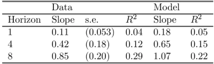
Proposition 3 (Coefficient in a predictive regression of stock returns via P/D ratios). Consider the predictive regression of the return from holding the stock from t to t+T, rt→t+T, on the initial log price-dividend ratio, ln (D/P)t:
Predictive regression: rt→t+T =αT +βT ln (D/P)t+noise (26) In the model, for small holding horizon T’s, the slope is, to the leading order:
βT = (ri+φH)T. (27)
where ri is stock’s effective discount rate (16), and φH is the speed of mean-reversion of resilience, hence of the P/D ratio. For the regression:
Predictive regression: rt→t+T =αT +β0T (D/P)t+noise (28) the coefficient is, to the leading order:
β0T = (1 +φH/ri)T. (29)
The intuition for (27) is the following. First, the slope is proportional to T, simply because returns over a horizon T are proportional to T. Second, when the P/D ratio is lower than baseline by x%, it increases returns through two channels: the dividend yield is higher by rix%— this is the ri term in (27); the price-dividend ratio will mean revert at a speed φ, creating capital gains ofφx%— this is the φH term in (27).
Using the paper’s calibration of ri = 5% and φH = 15%, Proposition 3 predicts a slope coefficient
Table 2: Predicting returns with Price-Dividend ratios
Data Model
Horizon Slope s.e. R2 Slope R2
1 0.11 (0.053) 0.04 0.18 0.05
4 0.42 (0.18) 0.12 0.65 0.15
8 0.85 (0.20) 0.29 1.07 0.22
Explanation: Predictive regressionEt[rt→t+T] =αT+βT ln (D/P)t, at horizonT (annual frequency). The data are Campbell (2003, Table 10 and 11B)’s calculation for the USA 1891—1997.
Nieuwerburgh (forthcoming), who find values of β1 between 0.23 in their preferred specification. Also, Cochrane (forth.) runs regression (28) at annual horizon, finds β01 = 3.8 with a standard error of 1.6. Proposition 3 predicts β01 = 4.
The same reasoning holds for other ratio of “fundamentals to prices.” For instance, in the model, the consumption / aggregate wealth (CAY) of Lettau and Ludvigson (2001) would have an expression:
CAYt =ri/
³
1 + Het
ri+φH
´
. Hence, CAY predicts future returns, as above In the regression: Et[rt→t+T] =
αT +βT lnCAYt, the coefficient is as in (27).
5.2
Cross-Sectional Predictability: Value and Growth Stocks
If a disaster happens, different stocks will fare differently.19 Their dividend will change byFt, the recovery rate. This dispersion of sensitivity of dividends to disasters leads to a dispersion of premia and prices in normal times. I propose that this might be a potential way to think about value and growth stocks (Fama French 1996, Lakonishok, Shleifer, Vishny 1994). In this rare-disaster interpretation, the value premium is compensation for “distress risk” (Fama and French 1996, Campbell, Hilscher, and Szilagyi forth.) due to the company’s behavior during economy-wide disasters.
I hasten to say that this subsection is arguably the most speculative of the paper. While Barro (2006) and Barro and Ursua (2007) have accumulated hard evidence for the importance of disasters, I know no positive evidence that value stocks do worse than growth stocks during disasters. Gourio (2007) presents some mixed evidence based on US data. It would be very good to have evidence for other countries, e.g. during World War II. But theorists have the license to speculate before the evidence is adduced. Also, with the “time-varying perception of risk” (rational or irrational) of disasters, we can use the model’s analytics to investigate the impact of “perception of risk” on cross-sectional prices and predictability.
First, consider the simple case of constant resilience, Ht≡H∗. Stocks with a low resilience are “risky 1 9For instance, stocks with a lot of physical assets that might be destroyed, or stocks very reliant on externalfinance, might have a lowerF.
”, as they will perform poorly during disasters. By Theorem 1, they have a low price/dividend ratio, i.e. they are value stocks. By Proposition 1, they have high returns — a compensation for their riskiness during disasters.
The same reasoning holds if resilience is stochastic.20 Stocks with a low resilience Hbt have a low P/D ratio, and high future returns. This also are value stocks.
The value spread forecasts the value premium So in the model, the value spread forecasts the value premium, as Cohen, Polk, and Vuolteenaho (2003) have found empirically. To see this in a simple context, consider a cross-section of stocks, with identical permanent resiliencesH∗. Say that at timet the support of their resiliences Hbt is [at, bt], where at < bt. Then, form a “Value minus Growth” portfolio, made of $1 of the extreme value stocks (low P/D), which correspond to Hbt=at, minus $1 of the extreme growth stocks (high P/D), which correspond to Hbt=bt. By Proposition 1, this portfolio has an expected return ofbt−at. On the other hand, the “value spread” in the P/D is: (bt−at)/[(ri+φH)ri]. The value spread is a perfect predictor of expected returns of a “Value minus Growth” strategy.
Under some simple assumptions, characteristics will predicts return better than covari-ances Suppose that a stock’s resilience is constant, i.e. Hbt≡0. In a sample without disasters, covariances between stocks are due to covariances between cash flows Dt in normal times. Hence, the stock market betas will only reflect the “normal times” covariance in cash flows. But risk premia are only due to the behavior in disasters, H∗. Hence, there will be no causal link between betas, stock market beta, and returns. The “normal times” betas could have no relation with risk premia. “Characteristics”, like the P/D ratio, will predict returns better than covariances.
However, there could be some spurious links if, for instance, stocks with lowH∗ had higher cash-flow betas. One could conclude that cash-flow beta commands a risk premium, but this is not because cash-flow beta causes a risk premium. It is only because stocks with high cash-flow beta happen to also be stocks that have a large loading on the disaster risk.21
With an auxiliary assumption, the model can also explain the appearance of a “value factor”, such as the High Minus Low (HML) factor of Fama and French. Suppose that resiliences have a 1-factor structure:
b
Hit=βHi HbM t+bhit 2 0
Fama and French (2007) show that the value premium is essentially due (at a descriptive level) to “migration”, i.e. mean-reversion in P/E ratio: a stock with high (resp. low) P/E ratio tends to see it’s P/E ratio go up (resp. down). It terms of the model, this means thatH∗is relatively constant across stocks, while thefluctuations inHetdrive the value premium.
2 1
Various authors (Julliard and Parker 2005, Campbell and Vuolteenaho 2006, Hansen Heaton and Li 2006)find that value stocks have higher long run cashflow betas. It is at least plausible that stocks that have high cash-flow betas in normal times also have high cash-flow betas in disasters, i.e. a lowFt and a lowHt. But is is their disaster-time covariance that creates a
where HbM t is a systematic (market-wide) part of the expected resilience of the asset, and bhit is the idiosyncratic part.
Consider two benchmarks. If for all stocks βHi = 1 (the “characteristics benchmark”) so that all dispersion in Hbi is idiosyncratic, then characteristics (the P/D ratio of a stock) predict future returns, but covariances do not. On the other hand, if for all stocksbhit≡0, but theβHi vary across stocks, all expected returns are captured by a covariance model. In general, reality will be in between, and covariances and characteristics are both useful to predict future returns.
These thought experiments may help explain the somewhat contradictory findings in the debate of whether characteristics or covariances explain returns (Daniel and Titman 1997, Davis Fama French 2000). When covariances badly measure the true risk (as in a disaster model), characteristics will often predict better expected returns than covariances.
6
Bond Premia and Yield Curve Puzzles Explained by the Model
In this section I show how the model matches key facts on bond return predictability.
6.1
Excess Returns and Time-Varying Risk Premia
We can now extract economic meaning from Proposition 2.
Bonds carry a time-varying risk premium Eq. 22 indicates that, bond premia are (to a first order) proportional to bond maturity T. This is the finding of Cochrane and Piazzesi (2005). The one factor, here, is the inflation premiumπt, which is compensation for a jump of inflation if a disaster happens. The model delivers this, because a bond of maturity T has a loading of inflation risk proportional to T.
The nominal yield curve slopes up on average Suppose that when the disaster happens, inflation jumps by j∗ > 0. This leads to the parametrization κ of the bond premia (Eq. 11) to be positive. The typical nominal short term rate (i.e., the one corresponding to it=i∗) is r=R−H$+i∗, while the long term rate is r+κ(i.e.,−limT→∞lnZt(T)/T). Hence, the long term rate is above the short term rate, by
κ >0.22 The yield curve slopes up. Economically, this is because long maturity bonds are riskier, so they command a risk premium.
2 2
6.2
The Forward Spread Predicts Bond Excess Returns (Fama-Bliss)
Fama Bliss (1987) regress short-term excess bond returns on the forward spread, i.e. the forward rate minus the short-term rate:
Fama-Bliss regression: Excess return on bond of maturity T =αT +βT ·(ft(T)−rt) +noise (30) The expectation hypothesis yields constant bond premium, hence predicts βT = 0. I next derive the model’s prediction.
Proposition 4 (Coefficient in the Fama-Bliss regression) The slope coefficient of the Fama-Bliss regres-sion (30) is given in (54) of Appendix C. When var(πt) À var(it)ψ2i (i.e., changes in the slope of the forward curve come from changes in the bond risk premium rather then changes in the drift of the short term rate),
βT = 1 + ψi 2 T+O
¡
T2¢ (31)
When var(πt) = 0 (no risk premium shocks), the expectation hypothesis holds, and βT = 0. In all cases, the slope βT is positive and eventually goes to 0,limT→∞βT = 0.
To see the economics, consider the variable part of the two sides of the Fama-Bliss regression (30). The excess return on T−maturity bond is approximately T πt (see Eq. 22), while the forward spread is
ft(T)−rt'T πt (see Eq. 25). Both sides are proportional toπtT. Hence, the Fama-Bliss regression (30) has a slope equal to 1, which is the leading term of (31).
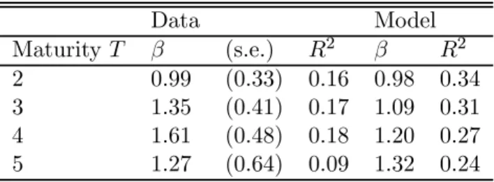
Table 3: Fama-Bliss Excess Return Regression
Data Model MaturityT β (s.e.) R2 β R2 2 0.99 (0.33) 0.16 0.98 0.34 3 1.35 (0.41) 0.17 1.09 0.31 4 1.61 (0.48) 0.18 1.20 0.27 5 1.27 (0.64) 0.09 1.32 0.24
Explanation: The regressions are the excess returns on a zero-coupon bond of maturityT, regressed on the spread between theT forward rate and the short term rate: rxt+1(T) =α+β(ft(T)−ft(1)) +εt+1(T). The unit of time is the year. The empirical results are from Cochrane and Piazzesi (2005, Table 2). The expectation hypothesis implies β= 0.
This is value βT = 1 is precisely what Fama and Bliss have found, a finding confirmed by Cochrane and Piazzesi (2005). This is quite heartening for the model.23 Table 3 reports the results. We see that indeed, to a good approximation, the coefficient is close to 1. We also see the rise of the coefficients with the maturity T, as predicted by Proposition 4.
Economically, the slope ofβT = 1, means that most of the variations in the slope of the yield curve are due to variations in risk-premium, not to the expected change of inflation.
6.3
The Slope of the Yield Curve Predicts Future Movements in Short and Long
Rates (Campbell Shiller)
Campbell and Shiller (CS, 1991) find that a high slope of the yield curve predicts that future long term rates will fall. CS regress changes in yields on the spread between the yield and the short-term rate:
Campbell-Shiller regression: yt+∆t(T−∆t)−yt(T)
∆t =a+βT ·
yt(T)−yt(0)
T +noise (32)
The expectation hypothesis predictsβT = 1. However, CS (see Table 4)find negativeβT’s, with a roughly affine shape as a function of maturity. This is what the model predicts, as the next Proposition shows.
Proposition 5 (Coefficient in the Campbell Shiller regression). The value of the slope coefficient, in the Campbell Shiller (1991) regression (32) is, when: φ2ivar(it)/var(πt)¿1, κ¿1:
βT = − µ 1 +2ψπ −ψi 3 T ¶ +o(T) whenT →0 (33) = −ψπT+o(T) whenT → ∞ (34)
Eq. (55) gives the exact expression for β.
Table 4 also simulates the model’s predictions. They are in line with CS’s results. To understand better the economics, I use a Taylor expansion, in the case where inflation is minimal. The slope of the yield curve is, to the leading order:
Slope of the yield curve≡ yt(T)−yt(0)
T =
πt
2 +O(T)
Hence, to a first order approximation (when inflation changes are not very predictable), the slope of the yield curve reflects the bond risk premium. Also, the change in yield is, (the proof of Proposition 5 justifies this) yt+∆t(T−∆t)−yt(T) ∆t '− ∂yt(T) ∂T = −πt 2 +O(T)
2 3Other models, if they have a time-varying bond risk premium proportional to the maturity of the bond, would have a similar success. So, the model illustrates a generic mechanism that explains the Fama-Bliss result.
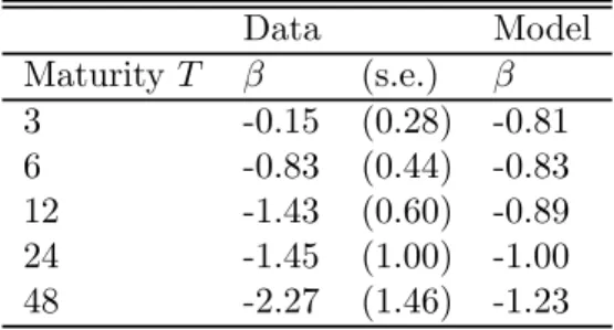
Table 4: Campbell-Shiller Yield Change Regression Data Model Maturity T β (s.e.) β 3 -0.15 (0.28) -0.81 6 -0.83 (0.44) -0.83 12 -1.43 (0.60) -0.89 24 -1.45 (1.00) -1.00 48 -2.27 (1.46) -1.23
Explanation: The regressions are the change in bond yield, on the slope of the yield curve: yt+1(T −1)−
yt(T) =α+ Tβ−1(yt(T)−yt(1)) +εt+1(T), The time unit is the month. The empirical results are from Campbell, Lo, MacKinlay (1997, Table 10.3). The expectation hypothesis implies β= 1.
Hence, the CS regression yields a coefficient of −1, to the leading order. Economically, it means that a high bond premium increases the slope of the yield curve (byπt/2).
At long maturities, Proposition 5 predicts that the coefficient in the CS regression becomes more and more negative. The economic reason is the following. For long maturities, yields have vanishing sensitivity on the risk premium (as in Dybvig, Ingersoll and Ross 1996), which the model says has the shape yt(T) = a+bπt/T +o(1/T), for some constants a, b. So the slope of the yield curve varies as
bπt/T2. But the expected change in the yield is −bφππt/T. So the slope in the CS regression (32) is
βT ∼ −φπT.
In Table 4, we see that thefit is quite good. The only misfit is at small maturity. The CS coefficient is closer to 0 than in the model. The short term rate has a larger predicable component, at short term horizons, than in the model. For instance, this could reflect a short-term forecastability in Fed Funds rate changes. That feature could be added to the model, as in section 9.2.2. Given the small misfit, it is arguably better not to change the baseline model, which broadly account for the CSfinding. Economically, the CS finding reflects the existence of a stochastic one-factor bond risk premium.
6.4
Cochrane and Piazzesi (2005)
Cochrane and Piazzesi (2005) deepen thefindings of Fama-Bliss and Campbell-Shiller. They establish that a parsimonious description of bond premia is given by one risk factor, such that a bond of maturity T has a loading proportional toT. Also, this risk premium is well-captured by a “tent-shape” of forward rates.
The theory in this paper yields theirfirstfinding. There is a single bond risk factorπt, which summarizes the behavior of inflation during disasters.
It also generates their second finding: the loading on the bond risk premium is proportional to the maturity, as per Eq. 22. Economically, it is because a bond of maturity T has a sensitivity to inflation
risk approximately proportional to T.
The theory has only two factors. So, there is no unique combination of yields that best captures the bond premium πt. However, simulations (not reported here), show that a “tent shape” factors−f(1) +
2f(3)−f(5)predict the bond premium with an accuracy close to that of an unconstrained combination.24 The reason for that is a transposition of an argument given first by Lettau and Wachter (2007): up to second order terms the combination −e−φif(1) +¡1 +e−φi¢f(3)−f(5) eliminates the it terms, and is
exactly proportional toπt. In any case, a conclusion is that the combination−f(1) + 2f(3)−f(5)(or any combination−f(a) + 2f(a+b)−f(a+ 2b)) is a good approximation of the risk premium. The extension in Proposition 9 allows to derive the optimal combination of yields to infer bond risk premia.
6.5
The Corporate Spread
Consider the corporate spread, which is the difference between the yield on the corporate bonds issued by the safest corporations (such as AAAfirms) and government bonds. The “corporate spread puzzle” is that the spread is too high, compared to historical rate of default. It has a very natural explanation under the disaster view. It is during disasters (in bad states of the world) that very safe corporations will default. Hence, the risk premia on default risk will be very high. To see this quantitatively, consider the case of short term debt securities. The spread for short term securities is:25
Corporate spreadt=ptEt
h
Bt+1−γFt+1$ (1−FCorp,t+1)
i
(35) To interpret this equation, consider the case where, conditional on default, all values are deterministic. Hence, when there is no expected nominal loss (during disastersFt+1$ = 1) the corporate spread is equal to the expected defaultpt(1−FCorp,t+1), times a risk-adjustment term equal toE
h
B−t+1γi. GivenEhBt+1−γi' 10 in the calibration, the model proposes why corporate spread is so high, compared to historical U.S. values (e.g. Huang and Huang 2003). The corporate sector defaults during very bad states of the world, so that risk-adjusted probability of default (pt) is ten times as high as than the physical probability of default
ptEt
h Bt+1−γ
i
. Hence the variable rare disaster model gives a microfoundation for Almeida and Philippon (2007)’s view that the corporate spread reflects the existence of bad states of the world.
This interpretation of the corporate spreads gives may explain Krishnamurthy and Vissing-Jorgensen (2007)’s finding, that when the debt/GDP ratio is high, the corporate spread is low — a finding for which their favored interpretation is a liquidity demand for treasuries. In the view of the present paper, one could say that, when Debt/GDP is high, the temptation to default via inflation (should a risk occur), is high, so
2 4The unconstrainedR2 is 25%, and the constainedR2is 21%.
2 5The yield on Government debt isR
−ptEtBt−+1γF$t+1
. CallingFCorp,t the recovery rate on a given corporation (e.g.,
the probability of survival to a disaster), the yield on Corporate debt isptEtBt−+1γF$t+1FCorp,t+1. So, the corporate spread
Ft+1$ is low, hence the corporate spread is low. Hence, the corporate spread is high when (i) the real risk is high: (i.a) put prices are high (so that FCorp,t+1 is low), (i.b) price/earnings ratios and market to book ratios are low (ii) and the nominal risk is low (Ft+1$ high): (ii.a) the Debt / GDP ratio is low, and (ii.b) the term premium is low.
6.6
Government Debt a
ff
ects Real Interest Rates, even under Ricardian Equivalence
The model allows to think about the impact of impact of the government Debt/GDP ratio. It is plausible that if the Debt/GDP ratio is high, then, if there is a disaster, the government will sacrifice monetary rectitude (that could be microfounded), so thatjtis high. That implies thatwhen the Debt/GDP ratio (or the government deficit / GDP) is high, then long-term rates are higher, and the slope of the yield curve is steeper (controlling for inflation, and expectations about future inflation in normal times). Dai and Philippon (2006) present evidence consistent with that view.
This effect works in an economy where Ricardian equivalent holds. Higher deficits do not increase long term rates because they “crowd out” investment, but instead because they increase the temptation by the government to inflate away the debt if there is a disaster, hence the inflation risk premium on nominal bonds.
Likewise, say that an independent central bank is a more credible commitment not to increase inflation during disasters (jt smaller). Then,real long term rates (e.g. nominal rates minus expected inflation) are lower, and the yield curve is less steep.
7
Options, Tail risk, and Equity Premium
Options offer a potential way to measure disasters. Hence, I provide a simple way to handle options in a variable disaster framework.
The price of a European 1-period put on a stock, with strike K, expressed as a ratio to the initial price, is (assuming no risk of default on the put — a surely too strong, but easily modifiable, assumption):
Vt=E ∙ Mt+1 Mt ³ K−Pt+1 Pt ´+¸ , where x+≡max (x,0).
Recall that, with LG processes, many parts of the variance of the processes need not be specified to calculate stock and bond prices. So, when calculating options, one is free to choose a convenient and plausible specification of the noise. Theorem 1 yieldedPt/Dt=a+bHbt, for two constantsaandb. Hence:
Et hP t+1 Pt |No disaster at t+ 1 i =eμ, witheμ≡ a+b e−φHHte 1+e−h∗Hte a+bHet e
gD. I propose to parametrize the stochasticity
according to: Pt+1 Pt = ⎧ ⎨ ⎩
eμ+σut+1−σ2/2 if there is no disaster at t+ 1 eμFt+1 if there is a disaster at t+ 1
0.95
1.00
1.05
1.10
Strike
0.18
0.20
0.22
0.24
0.26
0.28
0.30
Implied Volatility
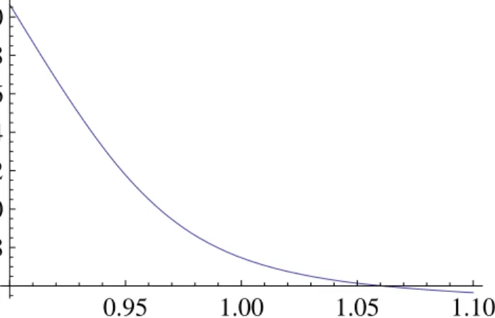
Figure 1: This Figures shows the Black-Scholes implied annualized volatility of a 1-month put on the stock market, using the model’s calibration. The initial value of the stock is normalized to 1. The implied volatility on deep out-of-the-money puts is higher than the implied volatility on at-the-money puts, which reflects the probability of rare disasters.
where ut+1 is a standard Gaussian variable. This equation means that, in normal times, returns are log-normal. However, if there is a disaster, the noise comes entirely from the disaster (there is no Gaussian
ut+1 noise). That choice will tidy up the option formula, it is economically meaningful: in a disaster, most of the option value comes from the disaster, not from “normal times” volatility.26
The above structure takes advantage of the flexibility in the modelling of the noise in Hbt and Dt. Rather than modelling them separately, I just assume that their aggregate, happens to give exactly a log normal noise.27 At the same time, (36) is consistent with the processes and prices in the rest of the paper.
Proposition 6 (Put price) The value of a put with strike K (the fraction of the initial price at which the put is in the money), with maturity next period, is Vt = VtN D +VtD, with VtN D and VtD the parts corresponding to the events with no disasters, and with disasters, respectively:
VtN D = (1−pt)e−R+μVP utBS ¡ Ke−μ, σ¢ (37) VtD = e−R+μptEt h Bt+1−γ ¡Ke−μ−Ft+1¢+ i (38) whereVBS
P ut(K, σ)is the Black-Scholes value of a put with strikeK, and volatilityσ, initial price 1, maturity 1, interest rate 0.
2 6The advantage of this discrete-time formulation is that, in the period, only one disaster happens. Hence, one avoids the infinite sums of the Naik and Lee (1990), which lead to infinite sums of the probability of 0,1,2... disasters.
Proposition 6 suggests a way to extract key structural disasters parameters from options data. Stocks with a higher put price (control for “normal times” volatility) should have a higher risk premium, hence higher future expected returns. Evaluating this prediction would be most interesting. Supportive evidence comes from Bollerslev and Zhou (2007). They find that when put prices are high, then subsequent stock market returns are high. Qualitatively, this is exactly what a disaster based model would predict. In a related way, high price of at-the-money options (as proxied by the VIX index) predicts high future returns (Giot 2005, Guo and Whitelaw, 2006). In ongoing work, Farhi and Gabaix (2007) extend the above formulation to a multi-country settings, and Farhi, Gabaix, Ranciere and Verdelhan (2007) investigate the link between currency options prices and currency levels. Early results are encouraging.
I now ask whether the model’s earlier calibration yield good values for options. I follow Du (2007), and calculate the implied Black-Scholes volatility for puts with a 1 month maturity. Du (2007) reports an average empirical values (using S&P 500 European options data from April 1988 to June 2005) the implied volatility of 29% is K = 0.92, and 20% for K = 1, the well-documented smile in options prices. Using the calibration of the rest of the paper, I find a volatility of 27% and 20% respectively for those maturities. Figure 1 reports the implied volatility. Hence, I conclude that, in a first pass, and for the maturity presented here, the variable rare disaster model gets correct options prices.28 Of course, a more systematic study would be desirable. At the same time, the “normal times” volatility is 14%. So the options-implied volatility is above the normal times volatility. Again, that simply reflects the fact that options prices are higher under the model than under Black-Scholes, because of the disaster premium.
8
Discussion
8.1
Cross-Asset Implications of the Model
The model allows to make cross-asset predictions, if we assume that the shocks to resilience are correlated across assets — for instance, that a shock that increases bond premia also increases stock premia.
When risk premia are high (high intensity of disaster, low Hbt, high πt): The slope of the yield curve is high (the bond premium is high); The price multiples (e.g. price / dividend, price / earnings, market to book ratio) of stocks are low; “Growth stocks” have a low P/E ratios; The value spread (e.g. measured as the difference of average market / book ratio, in the top quintile of its distribution, minus the bottom quintile) is low; Put prices are high, and options-based indices of Black-Scholes volatility (e.g., VIX) are high; The corporate bond spread is high.
2 8
I note that this conclusion is consistent with Du (2007), who calibrates a model with rare disasters and habit formation a la Menzly, Santos Veronesi (2004). As habit formation generates a high degree of risk aversion, he needs an intensity of disasters that is less than Barro (2006), actually about half as Barro: otherwise, he would get too high options prices. In my model, as the risk aversion is very moderate, the Barro c