Three Essays in Economics.

(1)

Three Essays in

Economics

by

Matthew George Hall

A dissertation submitted in partial fulfillment of the requirements for the degree of

Doctor of Philosophy (Economics)

in The University of Michigan 2016

Doctoral Committee:

Professor George A. Fulton, Co-Chair Professor Christopher L. House, Co-Chair Professor Charles C. Brown

Professor Susan M. Collins

(2)

c

Matthew George Hall 2016

(3)

(4)

ACKNOWLEDGEMENTS

I owe a debt of gratitude to my advisor, employer, co-chair, and friend George Fulton. Without his help I would never have been able to make the final push necessary to complete this dissertation. George is retiring next year, and the University of Michigan as well as the Research Seminar in Quantitative Economics will be poorer for it. George, thank you so much for everything.

I would also like to thank the other members of my committee, Christopher House, Charles Brown, Susan Collins, and Gabriel Ehrlich. I picked the easiest marks, the people who had never failed to help me when I asked for advice, or to listen when I requested their ear. Their willingness to sign up for this thankless task without hesitation, and on short notice, means the world to me.

For putting up with the aforementioned final push that lasted longer than I had any right to demand, and for the daily encouragement that made it bearable, I thank Jennifer Lambert.

My friends were a crucial support network in Michigan these years, both the ones who left and the one who stayed. I have made lifelong friendships with Collin Raymond, Christina DePasquale, Joshua Montes, and Ozan Jaquette. Josh did extra duty as a co-author, motivator, and informal advisor, for which he has my gratitude. My colleagues at RSQE, especially Joan Crary and Daniil Manaenkov, were a pleasure to work with and to learn from.

A special thank you is owed to my co-author, Aditi Thapar. Her willingness to communicate at all hours to meet my deadlines and to babysit me through learning Eviews were essential to the creation of a quality paper in a tight time frame.

David Ratner, Ryan Nunn, Adam Cowing, Seb Moosapoor, and Michigan resident Justin Gayle - you dragged me to the end. Thank you for everything, and I’ll see you in Vegas.

(5)

about that, but RSQE has the right man in the right job, and if it gets too crazy, just ask and I’ll be back to help.

Lastly, to my family - Barbara, Brad, Brian, Liz, Sam, Hannah, Shadow, and Maddie - thank you for everything. This was not easy, nor short. Thank you for noticing, and for refraining from making any jokes to that effect after year 7 or so. And thank you for believing this would always happen.

(6)

LIST OF FIGURES

Figure

1.1 Nominal Wage Changes in the PSID by Worker Category . . . 41

1.2 Nominal Wage Changes in the CPS by Worker Category . . . 42

1.3 Sources of Unemployment . . . 43

1.4 Labor Market Responses to Aggregate Productivity Shocks . . . 44

1.5 Nominal Wage Growth Among Job Stayers in the PSID by Year . . . 45

1.6 Nominal Wage Growth Among Job Switchers in the PSID by Year . . . 46

1.7 Nominal Wage Growth Among Job Finders in the PSID by Year . . . 47

1.8 Nominal Wage Growth Among All Workers in the CPS by Year . . . 48

1.9 Nominal Wage Growth Among Workers, Excluding Finders, in the CPS by Year . 49 1.10 Nominal Wage Growth Among Job Finders in the CPS by Year . . . 50

1.11 2-Year Nominal Wage Growth Among Job Stayers in the PSID by Year . . . 51

1.12 2-Year Nominal Wage Growth Among Job Switchers in the PSID by Year . . . 52

1.13 2-Year Nominal Wage Growth Among Job Finders in the PSID by Year . . . 53

2.1 Real-Time versus Current-Vintage Growth Rates . . . 74

2.2 IRFs in Response to 1 Percentage Point Increase in G . . . 75

2.3 IRFs of GDP in Response to 1 Percentage Point Increase in G . . . 76

2.4 IRFs of Private GDP in Response to 1 Percentage Point Increase in G . . . 77

2.5 IRFs of GDP Deflator in Response to 1 Percentage Point Increase in G . . . 78

(9)

3.1 Frequency of Charitable Contributions by Income Class . . . 116

3.2 Rate Effect of the AMT on Charitable Contributions . . . 117

(10)

LIST OF TABLES

Table

1.1 Descriptive Statistics . . . 33

1.2 Elasticity of Real Wages with Respect to Unemployment in the PSID . . . 34

1.3 Elasticity of Real Wages with Respect to Productivity in the CPS . . . 35

1.4 Measured Wage Rigidity in the PSID and CPS . . . 36

1.5 Empirical and Simulated Moments . . . 37

1.6 Model Parameters . . . 38

1.7 Elasticity of Real Wages with Respect to Individual Productivity in Simulated Data 39 1.8 Elasticity of Real Wages with Respect to Productivity, Unemployment (Simulated Data) . . . 40

2.1 Comparison of Real-Time Data for Variables of Interest . . . 82

2.2 VAR Specifications . . . 83

2.3 Forecast Error Statistics . . . 84

2.4 Cumulative Forecast Error Statistics . . . 85

2.5 Fiscal Multiplier of G on GDP . . . 86

2.6 Fiscal Multiplier of G on GDP . . . 87

2.7 Fiscal Multiplier of G on GDP, Instrument G with Defense Spending . . . 88

3.1 Descriptive Statistics . . . 119

3.2 Charitable Contribution, Itemizing Status, and AMT Status by Income Group . . 120

3.3 Building a Cross-Sectional Model of Charitable Giving . . . 121

(11)

3.5 Panel Model of Charitable Giving with Fixed Effects, Including AMT Indicator Variable . . . 123 3.6 Cross-Sectional Model of Charitable Giving, Including AMT Salience . . . 124 3.7 Panel Model of Charitable Giving with Fixed Effects, Including AMT Salience

Co-efficients are Uniform Across Income Classes . . . 125 3.8 Panel Model of Charitable Giving with Fixed Effects, Including AMT Salience

Non-Price Variables Vary Across Income Classes . . . 126 3.9 First-Stage Regression Results for Instruments . . . 127 3.10 Measurement Error in a Cross-Sectional Model of Charitable Giving . . . 128

(12)

CHAPTER I

Are Entry Wages Really (Nominally) Flexible?

1.1 Introduction

Downward nominal wage rigidity is often hypothesized to amplify unemployment fluctuations by constraining the responsiveness of wages to negative shocks. There is considerable evidence that the wages of incumbent workers are downwardly rigid, but the wages of new hires appear to be significantly more flexible. Because entry wages determine job creation over the business cycle, a substantial literature argues that downward nominal wage rigidity (hereafter, wage rigidity) is unlikely to explain unemployment dynamics.1

In this paper we argue that the apparent flexibility of entry wages is an artifact of selection bias. If unemployed workers are heterogeneous in their ability or willingness to reduce their reservation wages, those with more flexible reservation wages will be more likely to become re-employed. Because new hires will be disproportionately workers with flexible wages, the observed wages of new hires will appear flexible. The unobserved reservation wages of the workers who are not hired, however, may be quite rigid.

We estimate worker wage elasticities with respect to aggregate labor productivity and unemploy-ment in the Panel Study of Income Dynamics and the Current Population Survey. We confirm the

This chapter is co-authored with Gabriel Ehrlich and Joshua Montes. I would like to thank Charles Brown, Susan Collins, George Fulton, Christopher House, Pawel Krowlikowski, Ryan Nunn, David Ratner, and Matthew Shapiro for helpful comments. All errors are our own.

Disclaimer: The views expressed in this paper are the authors’ and should not be interpreted as the views of the Congressional Budget Office.

(13)

consensus in the literature that wages appear to be more elastic for new hires than for incumbents. We contrast this evidence with histograms of nominal wage changes from the same survey data, which exhibit substantial downward nominal wage rigidity in all years for both long-time workers (hereafter job stayers) and for workers with recent spells of non-employment (job finders).

We construct a search and matching model of the labor market and show that hiring wages can appear flexible even if unemployed workers’ reservation wages are quite rigid. We estimate the parameters of the model using indirect inference and find substantial nominal rigidity for both job stayers and finders. Using simulated data from the estimated model, we show that the elasticities of observed wages closely resemble those in the data for job stayers and job finders: finders display more elastic wages than stayers. Those elasticities are not targets of the model estimation. The model’s ability to generate disparate wage elasticities among job stayers and job finders stems naturally from the selection bias inherent in conditioning the sample on observed wages. Pooling unemployed workers’ reservation wages with the observed wages of job finders brings the elasticity of the wages of potential new hires substantially closer to that of job stayers.

Dynamic simulations of the model clarify the mechanisms by which aggregate observed wages appear more responsive to labor market conditions than the underlying levels of wage rigidity would imply. Although the observed wages of job finders fall sharply in response to a negative shock, the reservation wages of unemployed workers remain rigid. This asymmetry highlights the pitfalls of selecting on successful job finding to measure wage responsiveness to aggregate economic conditions among potential new hires. Layoffs rise immediately in response to a negative shock, followed by a persistent decrease in the job finding rate, the majority of which can be attributed to the rigid reservation wages of unemployed workers. The importance of wage rigidity in our model to flows out of unemployment re-establishes its potential as an explanation for observed unemployment volatility. At least since Shimer’s (2005) demonstration that the canonical search and matching model of the labor market with perfectly flexible wages cannot replicate the observed volatility in unemployment, a large literature has explored whether adding some form of wage rigidity can help to reconcile the model to the data. Prominent examples include Hall (2005), who introduces real wage rigidity via

(14)

a bargaining norm between workers and employers, Gertler and Trigari (2009), who model wage bargaining with staggered multi-period contracts, and Christiano et al. (2015), who endogenously derive wage rigidity from alternating offers in bargaining negotiations.

Several empirical studies, however, show that the wages of new hires are much more responsive to labor market conditions than the wages of longer-tenured workers. Bils (1985), Shin (1994), Solon et al. (1994), Devereux (2001), and Shin and Solon (2006) all find lower elasticities of wages with respect to the unemployment rate for tenured workers than for all workers. Bils (1985), Shin (1994), and Barlevy (2001) find specifically that the elasticity for those in new matches is much higher than the estimates for incumbent workers. Furthermore, Haefke et al. (2013), after correcting for composition bias in worker subgroups, obtain much higher elasticities in the aggregate wages of new hires with respect to average labor market productivity than for the worker population generally. As Pissarides (2009) summarizes the evidence, “Time-series or panel studies on the cyclical volatility of wages show considerable stickiness, but this evidence is dominated by wages in ongoing jobs and is not relevant for job creation in the search and matching model.”2

Notably, the time series evidence contrasts starkly with the direct survey evidence on unemployed workers’ reservation wages reported by Krueger and Mueller (2014). They find that “...self-reported reservation wages decline at a modest rate over the spell of unemployment...” They argue that their evidence suggests that “...many workers persistently misjudge their prospects or anchor their reservation wage on their previous wage.” We argue that a model with heterogeneity in the rigidity of unemployed workers’ wages resolves the apparent contradiction between these two sources of evidence.

The remainder of the paper proceeds as follows. In section 1.2, we establish within two different data sources the key empirical elasticities regarding entry wage rigidity. In section 1.3 we employ those same data sources to provide evidence in favor of wage rigidity for both job stayers and job finders. In section 1.4 we introduce a labor search model with explicit downward nominal wage

2_{Elsby et al. (2013) are also skeptical of the role that downward nominal wage rigidity plays in unemployment} fluctuations. They find a significant number of nominal wage cuts in CPS data and point out that in the Great Recession the most notable distinction from previous contractions, which occurred in times of higher inflation, is not in separations but in the duration of unemployment. This result puts the onus on entry rigidity to explain the data, a hypothesis for which they find little theoretical and no empirical support.

(15)

rigidity for all workers. In section 3.5 we estimate the model and illustrate the results. Section 1.6 concludes.

1.2 Elasticities for Job Stayers, Switchers, and New Hires

Our empirical analysis utilizes longitudinal data from two sources, the Panel Study of Income Dynamics (PSID) and the Current Population Survey (CPS). We use the PSID to conduct analyses similar to those in Solon, Barsky, and Parker (1994) and Devereux (2001), in which we estimate the elasticities of the real wages of job stayers and all employed workers with respect to the unemployment rate. We use the CPS to estimate the elasticity of real wages of all workers and job finders with respect to average labor productivity, in the spirit of Haefke et al. (2013). In both cases, we confirm the qualitative patterns in the original studies: the wages of job stayers are less responsive to the unemployment rate than are the wages of all workers, and the wages of job finders are more responsive to labor productivity than are the wages of all workers.

1.2.1 Panel Study of Income Dynamics

The PSID contains data on employment, salary, and hourly wages for household heads and their spouses. We combine the 1980-1997 annual surveys with the 1999-2013 biannual surveys to construct an employment history for respondents that spans from 1980-2013.3 _{The number of respondents in}

these surveys averages about 12,500 per year.4 The PSID includes occupational codes and industry codes, as well as job start and end dates, which allows us to determine worker tenure over several years.

Table 1.1 provides a summary description of some key variables in the analysis. About 24 percent of those surveyed are salaried workers, while almost 35 percent are hourly employees. The remainder is disproportionately retired or otherwise out of the labor force. Our analysis focuses on hourly workers, for whom we have wage data, and salaried workers, for whom we construct an

3_{We begin the analysis in 1980 because hourly wages are top-coded at very restrictive levels in the 1978 and prior} surveys.

4_{We include spouses in the analysis when we consider the entire universe of working adults. The inclusion of} spouses is necessary to ensure that the primary earner in a family is present in the analysis because the PSID codes household heads by gender. We also include some results that are restricted to male heads of household to facilitate comparisons with past studies. That restriction does not change the qualitative results.

(16)

hourly wage. Most salaried workers do not provide a consistent measure of hours for their primary job, so we assume a fixed number of hours from year to year; this assumption seems reasonable for those who stay at the same job from one survey to the next (about 66 percent of salaried workers), but potentially biases the hourly wage for those who switch jobs.

We categorize the set of employed workers as job stayers, job switchers, and job finders.5 _Job

stayers are defined as workers who provided a start date at their current job prior to the last time they were surveyed, when available, or who provided a tenure length at their current employer exceeding the time between survey dates if the start date is unavailable. In addition, job stayers must have had continuous employment between survey dates without spells of unemployment or time out of the labor force. Job switchers are defined as workers who maintained continuous employment, defined by no months in which they were unemployed or out of the labor force, but who provided a start date between survey dates. Job finders are defined as workers who were employed at the time of both the current and prior surveys, but who report having spent time between surveys as either unemployed or out of the labor force.6

We estimate regressions of the form:

∆ lnwit=β0+β1t+β2∆Ut+β3Xit+εit, (1.1)

in which wit is the nominal hourly wage, Ut is the national unemployment rate, and Xit is a

polynomial measure of work experience and job tenure for worker i at year t. These regressions follow Devereux (2001), who in turn builds on Solon et al. (1994). We use both the dependent variable in Devereux (2001), which is limited to earnings in the worker’s primary job, as well as that in Solon et al. (1994), who use all earnings in the surveyed year. In addition, although Solon et al.

5_{Although our categorization involves some subjective judgment, which may induce misclassification, we will} clas-sify workers using identical definitions in our estimation of the theoretical model. This method of indirect inference allows us to correct for possible misspecification in these definitions. See section 1.5.1 for more details. Our catego-rization is a partition of all workers who have valid wages in consecutive surveys.

6_{Note that this definition excludes first-time entrants and re-entrants who spent multiple years unemployed or} out of the labor force. Before concluding this section, we want to reiterate that in both datasets our definition of job finders excludes new entrants to the labor market. According to our CPS dataset, over the past 20 years, new entrants constitute between 6-12 percent of the unemployed looking for work and average only 8.6 percent of the total unemployed during that time.

(17)

(1994) include only men, we include both men and women in our sample.7

Table 1.2 presents the results of our regressions. Although our sample periods differ, and our inclusion of women alters our sample slightly compared to Solon et al.’s, our analysis recovers the same basic fact pattern as the earlier studies. When we confine our sample to the years in which we have annual surveys (1980 to 1997), we estimate that the elasticity of all wages with respect to the annual unemployment rate is -0.83, versus -0.55 for job stayers. When we extend the analysis to include job switchers and job finders, we estimate elasticities of -1.80 and -1.82, respectively, far larger (in absolute value) than for all workers or job stayers. Extending the sample forward in time to incorporate the biannual surveys from 1999 to 2013 yields uniformly smaller elasticities, but the relative magnitudes among all workers, job stayers, and job finders are unaffected.

Our specifications using the average annual wage give similar qualitative results. When we end the sample at 1997, we estimate that the elasticity of real wages with respect to unemployment is -0.7 for all workers and -0.49 for job stayers. When we analyze job finders separately, we estimate an elasticity of -1.65, consistent with the notion that job finders’ wages are more responsive to labor market conditions than the wages of other workers. When we extend the sample to include years through 2013, we see somewhat higher elasticities, but the relative magnitudes among all workers, job stayers, and job finders are unaffected.

1.2.2 Current Population Survey

The CPS’s outgoing rotation group includes data on wages and weekly hours worked for all members of a household, job codes, and demographic information, along with data from the basic monthly files that include the employment history of each household member. We use the merged datasets of Drew et al. (2014), who build on the methodology of Madrian and Lefgren (2000) to link CPS responses from the same individual longitudinally for up to 16 months, the maximum time that individuals are covered by the survey. The structure of the CPS is such that individuals are surveyed for four consecutive months, are out of the survey for eight months, and then are surveyed again

7_{Both papers use a two-step process to address potential bias in their standard errors due to common time effects} across workers. We address this issue by clustering standard errors by year and estimate the regression in equation 1.1 directly.

(18)

for four more months. This design allows us to construct a year-over-year measure of wage changes for individuals in the outgoing rotation groups. We combine the 1989-2013 monthly surveys with aggregate labor market data such as the unemployment rate, labor productivity, CPI-U measure of inflation, and the private consumption implicit price deflator.

Following the procedure of Haefke et al. (2013), we restrict the dataset to nonfarm, nonsuper-visory, private-sector workers, trim outliers in hours worked and in implied hourly earnings, impute top-coded earnings according to the procedure in Schmitt (2003), and use typical hours worked per week as our divisor in the determination of the hourly wage for salaried workers.8 We construct a variable for years of school and a standard measure of potential experience (age minus years of school minus 6). Finally, we include dummy variables for female, black, Hispanic, and married with spouse present in our list of covariates.

Haefke et al. (2013) investigate the effect of changes in productivity on aggregate real wages of both job finders and all workers. To account for composition bias in each group, they remove demographically explainable wage determinants for all workers via a Mincer regression, and then analyze the effects of labor market indicators on the respective residualized aggregate wages. They define a job finder, or new hire, as any worker who had an unemployment spell in the prior 3 months. We adopt that definition of a job finder in the CPS, as we do not have employment information for the 8 months prior to those 3.9 _{Therefore, our definition of job finder is more restrictive in the}

CPS than in the PSID, which allows for the measurement of nonemployment spells further from the survey date.

Haefke et al. (2013) estimate the following specification by quarter for each subgroupjof workers from 1984 to 2006:10

∆ lnwjt=β0,j +β1,j∆ lnyt+εjt, (1.2)

8_{In contrast, Card and Hyslop (1997) and Elsby et al. (2013) use usual weekly earnings for salaried workers.} 9_{See Drew et al. (2014) for a detailed discussion of the structure of the CPS.}

10_{They exclude 1995q3 and 1995q4 from analysis because of a change in sample design that makes it difficult to} match workers, add quarter dummies to account for residual seasonality, and add a dummy for 2003q1 to reflect the change in occupation classification in 2003 that increases the fraction of supervisory workers.

(19)

wherewjt is their residualized real wage series for groupj andytis a measure of labor productivity.

Haefke et al.’s preferred specification deflates wages by the BLS private nonfarm business sector implicit deflator and uses aggregate labor productivity as their aggregate labor market indicator of interest.11

We follow the spirit of Haefke et al.’s analysis, with the major exception that we use the lon-gitudinal aspect of the CPS to calculate the year-over-year change in wages for individual workers and use those changes as the outcome of interest in our analysis. We choose this approach over the residualization approach of Haefke et al. (2013) because it is more consistent with our analysis using the PSID data and because using within-worker wage changes corrects for unobservable com-positional changes among worker groups in addition to observable ones. On the other hand, this approach restricts the sample of workers who could potentially be considered new hires, and requires year-over-year as opposed to quarter-over-quarter comparisons. This restriction also means that we include individuals only once, the second time they reach the outgoing rotation group. Additionally, we use the private consumption deflator as our measure of inflation (using the CPI-U has almost no effect on the results). We therefore run the following regressions for job finders and all workers:

∆ lnwijt=β0,j+β1,j∆ lnyt+β2,jXit+εit, (1.3)

where an observation is a workeriin worker groupjand calendar quartert, and the first difference terms represent year-on-year changes. Xit is a cubic polynomial in experience, consistent with our

analysis using the PSID data.

Table 1.3 presents the results of our regressions, along with some key results from Haefke et al. (2013) for comparison. Whereas Haefke et al. (2013) estimate that the elasticities of the real wages of all workers and job finders with respect to average labor productivity are 0.24 and 0.79, respectively, we estimate those elasticities as 0.29 and 0.55. Part of the reason that we estimate a lower elasticity for job finders is our inclusion of more recent calendar years, which in our analysis

11_{The aggregate labor productivity series published by the Bureau of Labor Statistics has been revised subsequent} to the publication of their paper, which complicates the comparison of our results to theirs.

(20)

of the PSID data led to less estimated responsiveness of wages to labor market conditions.

Overall, we view our results as qualitatively similar to Haefke et al.’s: the wages of new hires are more responsive to productivity changes than are the wages of all workers.12 _{More broadly, the}

estimates in this section confirm the key patterns in the literature: the observed real wages of job finders are roughly twice as responsive to changes in labor market conditions as the real wages of all workers, which are themselves more responsive than the wages of job stayers.

1.3 Estimating Downward Nominal Wage Rigidity for Job Stayers, Job

Switchers, and New Hires

In this section, we employ a complementary approach to those in section 1.2 to measuring wage rigidity. We focus particularly here on downward nominal wage rigidity by attempting to measure the proportion of wage cuts that would have occurred in a counterfactual environment with perfectly flexible wages that are “missing” from the observed data. We estimate this proportion using the method in Ehrlich and Montes (2014), which builds on the method of Card and Hyslop (1997). The essence of the method is to extrapolate from the upper half of the observed wage change distribution to what the nominally negative portion of the distribution would look like in the absence of rigidity, and calculate the proportion of counterfactual mass that is missing in the observed distribution.13

Although such analyses have typically focused on the wages of job stayers, the same method can be extended to job switchers and job finders, as shown in the subsections below.

The key results that emerge from performing this analysis in the PSID and CPS are that the observed wages of job finders exhibit less downward nominal wage rigidity than the wages of job stayers, but the degree of rigidity in job finders’ wages is nonetheless substantial. We begin this section by describing the visual evidence for wage rigidity in the PSID and CPS, before providing formal estimates of the degrees of nominal rigidity.

12_{Again, we note that our definition of new hires is restricted to workers who were employed one year previously,} which is not the case for Haefke et al. (2013).

(21)

1.3.1 PSID

Our longitudinal dataset using survey data from the PSID includes 144,047 observations of (constructed) hourly wage data matched to the same worker in consecutive surveys over 25 surveys, the majority of the observations being job stayers. Figure 1.1 illustrates these data in histograms of one-year and two-year percent wage changes for job stayers, job switchers, and job finders for survey years 1980-2013. The histograms are truncated at -50 and 50 percent, with a dotted vertical line to indicate a zero percent nominal wage change.14

The first row of histograms in figure 1.1 contain a spike in the proportion of reported wage changes at nominal zero, which we interpret as one of the hallmarks of downward nominal wage rigidity. There is also a visually evident asymmetry between the nominally positive and nominally negative portions of the distribution, as the proportions of nominally negative wage changes are smaller than a simple extrapolation from the nominally positive portion of the distribution would indicate. This asymmetry is especially evident in the 2-year changes in the histogram for job stayers, which contain sample years with lower inflation, among other factors, leading to smaller nominal wage increases. Negative wage changes have nevertheless remained relatively uncommon; thus, the distribution of wages has “piled up” against the barrier at nominal zero.

The second and third rows of figure 1.1 show similar histograms for job switchers and job finders, respectively. The dispersion of wage changes is higher for both job switchers and job finders than for job stayers. Furthermore, the median wage change for job finders, at 3.7%, is lower than for job stayers, which is 4.6%. Nevertheless, the histograms share significant similarities with those for stayers: 1) a spike at nominal zero, and 2) asymmetry between the nominally positive and nominally negative portions of the wage change distribution. There is less mass in the nominally negative portion than would be implied by a symmetrical wage change histogram, consistent with the idea that the wages of job switchers and job finders exhibit some degree of downward nominal rigidity.

14_{Individual-year histograms of wage changes for stayers, switchers, and finders are also shown in the appendix.} Each year exhibits the same basic pattern, with a spike at nominal 0 wage change.

(22)

1.3.2 CPS

Figure 1.2 provides wage change histograms for all workers, all workers excluding job finders, and job finders only in the CPS outgoing rotation groups for the years 1989 to 2013. We censor the histograms at -80% and 80% because the sample sizes are larger than in the PSID.15 _{The sample}

is limited to those workers who can be matched between their 4th and 16th months in the survey. We divide these workers into job finders and non-job finders, a combination of job stayers and job switchers, as described in section 1.2.2. There are 23,600 total wage changes on average per surveyed year, of which approximately 900 per year come from workers we classify as job finders.

The histograms in figure 1.2 are qualitatively similar to those in figure 1.1. There are large spikes at nominal zero and an asymmetry between the nominally positive and negative portions of the distributions, with the latter displaying “missing” mass. Again, the wage change distributions of job finders display weaker, but still suggestive, evidence of downward nominal rigidities than the distributions for other workers.

1.3.3 Systematic Measurement of Wage Rigidity

In this section we provide formal estimates of the proportion of nominal wage cuts that would have occurred in an environment with no nominal wage rigidity that are instead prevented by downward nominal wage rigidity. The basic approach, described in detail in the appendix, is to construct an empirical distribution of log nominal wage changes and reflect the 50-100th percentile of changes back on the 0-50th percentiles. The implied share of nominal wage cuts that would be expected based on the upper half of the wage change distribution is compared with the actual share of nominal wage cuts. The statistic:

c

wr= 1−Fˆ

obs₍₀-₎

ˆ

Fcf₍₀-₎ (1.4)

15_{Year-by-year histograms for each category of worker are found in the appendix. The histograms for 1995 are} omitted because a change in sampling design does not permit matches of worker wages to their employment history.

(23)

represents the fraction of wage changes that are “missing”, where ˆFcf(0-) is the estimated coun-terfactual distribution of log wage changes and ˆFobs₍₀-_{) is the empirical distribution of log wage}

changes.

This statistic reflects the combination of two phenomena associated with downward nominal wage rigidity. First, it captures the extent to which slightly negative nominal wage changes are “swept up” to nominal 0. Second, it may also capture the share of workers who would have received a wage cut in an environment with flexible wages but who instead separated from their employer either through a layoff or a quit.

Table 1.4 displays our estimates of the proportion of nominal wage cuts prevented by wage rigidity both in the PSID and in the CPS. The table presents estimates for the PSID for job stayers, job switchers, and job finders for the years 1980 to 2013, and for the CPS for all workers, non-job finders, and job-finders for the years 1989 to 2013. The table also displays separate estimates for salaried and hourly workers.

We estimate that 52.7% of counterfactual nominal wage cuts are missing among job stayers in the PSID, versus 56.1% and 36.4%, respectively, for job switchers and job finders. The estimates for salaried and hourly workers do not differ systematically: salaried job stayers display less wage rigidity than hourly job stayers, but salaried job switchers and finders display more wage rigidity than their hourly counterparts.

The estimates using the CPS data are qualitatively similar. We estimate that among all workers, 47.4% of counterfactual nominal wage cuts were prevented by wage rigidity, versus 38.6% for job finders. Again, the estimate for salaried and hourly workers do not vary in a consistent fashion.

One potential limitation of using reported survey data on nominal wages over time to estimate wage changes is that respondents may round their hourly wage to the nearest dollar or half dollar, or their salary to the nearest 1000 dollar value.16 _{This rounding could lead to an overstatement of}

the number of unchanged nominal wages from year to year. An inflated number of unchanged wages could bias our measure of rigidity if small wage cuts disappear due to rounding. To examine the

(24)

potential effect such rounding has on our results, we re-estimate wage rigidity for hourly workers after excluding all round-dollar results (about one third of the sample for incumbents and finders, slightly less for switchers). Reassuringly, the percent of counterfactual wage cuts prevented by wage rigidity decreases only from 55.1% (see table 1.4) among job stayers to 53.6%, with that third of respondents excluded from the analysis, while rigidity among job switchers declined from 50.2% to 48.4%. Finders registered a wage rigidity measure of 35.4%, versus 36.6% including the entire sample of hourly employees.

We interpret these estimates as indicating a substantial amount of downward nominal wage rigidity for workers in the United States economy. Importantly, although the wages of job finders appear to exhibit less rigidity than the wages of other workers, they are by no means perfectly flexible. Therefore, these results stand in some contrast to the results in section 1.2, which indicated much more responsiveness of the wages of job finders to labor market conditions than the wages of job stayers. In the next section, we build a search and matching model of the labor market that attempts to reconcile these results, and implies that the apparent flexibility of the wages of job finders stems from composition bias in the pool of newly hired workers.

1.4 Model

We consider a general equilibrium model with search and matching in the labor market that is closely related to the canonical model of Mortensen and Pissarides (1994). However, we model wage setting differently than those authors do. We assume, as in Barattieri et al. (2010) and Daly and Hobijn (2014), that workers set their wages unilaterally. We further follow Daly and Hobijn (2014) by adopting a Calvo-style (1983) process: we assume that in any given period, a fraction of workers are constrained from reducing their nominal wages. The model allows the fractions of employed and unemployed workers who are prevented from reducing their wage demands to differ.

(25)

1.4.1 Model Environment

We consider the stationary equilibrium of a discrete time model with no aggregate shocks but with shocks to a worker’s idiosyncratic productivity and their ability to reduce their nominal wage demands each period. Each firm has one job, which can either be vacant or filled and producing output. There is a unit mass of workers who can be either employed in a job or unemployed and searching for a job.

Firms and workers are infinitely lived with a common discount rateβand have linear preferences over profits and consumption, respectively. Workers and firms cannot store goods, thus workers consume their entire incomes each period. There is also no intensive margin of labor supply: workers in a filled job supply exactly one unit of labor, L, each period. Unemployed workers receive an unemployment benefitb each period.

Firms in a match with a worker can decide whether to continue to employ the worker at the worker’s demanded wage or to terminate the job. Labor is the only input into production, and the output of a filled job is given by:

Y =pL=p (1.5)

where pis stochastic and can be conceptualized either as the productivity of a worker or the price of a job’s output. We refer to pas productivity in this paper. The per-period profitsπ of a firm with a worker with productivitypand paying wageware then:

π(p, w) =p−w. (1.6)

Firms that are not in a match and wish to meet with a worker must post a vacancy at per-period costc, expressed in units of output. There is free entry into vacancy posting.

Unemployed workers and firms with vacant jobs form matches according to a matching function

m(v, u), wherevis the number of vacancies anduis the number of workers who are unemployed.17

(26)

We assume that the matching function has the Cobb-Douglas form:

m(v, u) =Avφu1−φ (1.7)

where A is a parameter that governs matching efficiency and φ is the elasticity of the matching function with respect to the number of vacancies. Denoting ‘labor market tightness’v/uas θ, the probability f that a worker meets a vacancy is f(θ) =m(v, u)/u=Aθφ_{. The probability}_q _{that a}

firm with a vacant job meets an unemployed worker isq(θ) =m(v, u)/v=Aθφ−1.

There is no on-the-job search, and matches end with exogenous probability sx each period.

Endogenous separations occur in two ways. First, matches end when the productivity level of the match falls to a low enough level that the match surplus between the worker and firm is exhausted. Those separations are bilaterally efficient. Second, bilaterally inefficient separations occur when the worker is unable to cut his or her nominal wage demand below the maximum level that the firm is willing to pay, but would have been willing to do so in an environment with flexible wages.

We model wage rigidity according to the process in Calvo (1983). Employed and unemployed workers set their reservation wages unilaterally. We assume employed and unemployed workers are unable to reduce their wage demand in any given period, with probabilitiesλEandλU, respectively.

Firms then decide whether to continue or to terminate matches given workers’ wage demands. The timing of each period is as follows:

1. The period begins and employed and unemployed workers draw realizations of whether they can reduce their reservation wages in the period.

2. Workers draw their idiosyncratic productivity levels, and firms and workers observe workers’ productivity levels.

3. Firms post vacancies and matching between vacancies and unemployed workers occurs. Not every match between an unemployed worker and a vacancy will result in the formation of a new job both because of exogenous separations and because the worker’s wage demand may be higher than the firm will accept. To distinguish between a match and a new employment relationship that enters production, we will call a match between an unemployed worker and a vacant job aninterview. The probabilitiesf andqare the likelihoods of an unemployed worker receiving an interview in a given period and of a firm that has posted a vacancy interviewing a worker, respectively.

4. Exogenous separations occur.

(27)

Note that exogenous separations can occur even in new interviews, such that the worker is never employed by the firm regardless of productivity levels or wage demands.

5. Workers in a negotiation set their wage demands, while unemployed workers re-set their reser-vation wages.

6. Firms decide whether to accept matched workers’ wage demands and proceed to production, or to terminate the relationship.

We will refer to the process of workers setting their wage demands and firms deciding whether to accept them as a negotiation, although there is no actual bargaining involved. Note that from the firm’s perspective, there is no difference between a negotiation with a previously unemployed worker and a worker in an ongoing employment relationship. Therefore, we will not generally distinguish between the two.18

7. Production occurs, wages and unemployment benefits are paid, profits are earned, and con-sumption occurs.

8. The period ends.

Firms can therefore be in two different states, with an unfilled vacancy or in a match with a worker. We will denote the values to the firm of being in these states as V and J, respectively. Workers can find themselves in four possible states: unemployed with a flexible wage, unemployed with a rigid wage, employed with a flexible wage, and employed with a rigid wage. We will denote the values of the worker to being in these states asUF_,_UR_, _WR_{, and}_WF_{, respectively. We define}

the value functions for these states in sections 1.4.2 and 1.4.3.

We assume that a worker’s log productivity follows the AR(1) process:

lnp= (1−ψp) ln ¯p+ψplnp−1+εp, εp∼N 0, σ2p

. (1.8)

Productivity is a time-varying, mean-reverting characteristic of the individual worker. Further, a worker’s productivity process persists in unemployment. The productivity distribution of employed workers will differ from the distribution for all workers because firms will lay off workers when their reservation wages exceed the cutoff value associated with the worker’s productivity.19

1.4.2 Firm’s Problem

The value to the firm of posting a vacancy, denoted V, is defined in step 3 in the timeline and given as:

V =−c+q(θ)(1−sx)

Z Z

J(p, w) dG(p, w) + (1−q(θ)(1−sx))βE[V0], (1.9) 18_{The distinction does matter for calculating employment flows such as job creation and job destruction.}

19_{It is unnecessary that a worker’s productivity level be higher than the worker’s wage in every period due to the} associated option value of a match.

(28)

whereG(p, w) is the stationary joint cumulative distribution of productivity levels and wage demands from unemployed workers. The firm incurs the flow costcof posting a vacancy and gains the expected value of a negotiation with probabilityq(θ)(1−sx), which accounts for both the likelihood of a match

and its survival to become a negotiation, as well as the continuation value of the vacancy conditional on not matching.

The value to the firm of being in a negotiation with a match of productivity p and worker reservation wagew, denoted by J and defined in step 6 in the timeline, is given by:

J(p, w) = max discontinue,continue n βE[V0], p−w+β(1−sx) Z Z J(p0, w0) dF(p0|p)dH(w0|p0, w)o. (1.10)

The firm decides between terminating the match or entering into production with the matched worker. In production the firm receives the flow surplusp−wand the expected continuation value of a filled job conditional on the current period’s wage and productivity (inclusive of the risk of an exogenous separation during negotiation next period). F(p0_|_p_{) is the cumulative distribution} function of next period’s productivity level given this period’s productivity, andH(w0|p0, w) is the cumulative distribution function of next period’s wage demands for a worker in a filled job given current wagewand next-period’s productivity levelp0.20

Given equation 1.10, we can define the wage for which the firm is indifferent between continuing and terminating the employment relationship. That cutoff wage, denoted as ˜w(p), is a function of productivity and solves the equation:

βE[V0] =p−w+β(1−sx)

Z Z

J(p0, w0) dF(p0|p)dH(w0|p0, w). (1.11)

1.4.3 Worker’s Problem

We define the worker’s value functions as of step 5 in the model, after matching and exogenous separations have occurred, when the worker must decide his or her reservation wage. The value of being in a negotiation with a flexible wage is a function of this period’s productivity level, and we denote itWF(p). The value of being in a negotiation with a rigid wage depends on both this period’s productivity and last period’s wage demand, and we denote itWR(p, w−1). It is sometimes

convenient to represent expectations of next period’s value of being employed, without knowing

20_{The expected value of a match next period can be further decomposed based on the probability of wage adjustment} next period, but we omit that characterization here.

(29)

whether the worker’s wages will be flexible or rigid. We denote this expectation asE[W(p0, w)] =

E[(1−λE)WF(p0) +λEWR(p0, w)].

Likewise, the value of being unemployed in step 5 with a flexible reservation wage is a function of this period’s productivity only, so we denote it UF₍_p_{). The value of being unemployed with a}

rigid reservation wage is a function of this period’s productivity and last period’s wage demand, so we denote it UR₍_{p, w}

−1). When we wish to denote the expected value of being unemployed next

period, we use the notationE[U(p0, w)] =E[(1−λU)UF(p0) +λUUR(p0, w)].

The value to the worker of being in a negotiation with a flexible wage and productivitypis given by:21 WF(p) = max w 1(w≤w˜(p))w+β Z (1−sx)E[W(p0, w)] +sxE[U(p0, w)] dF(p0|p) +1(w >w˜(p)) b+β Z f(θ)(1−sx)E[W(p0, w)] + (1−f(θ)(1−sx))E[U(p0, w)] dF(p0|p) . (1.12)

The worker chooses his or her wage demand w knowing the firm’s cutoff wage given the current productivity level ˜w(p). Choosing a wage demand lower than that cutoff, as in the first term of the value function, yields the demanded wage this period and a continuation value associated with starting the next period in an ongoing match with the firm. Choosing a higher wage leads to a termination of the match, yielding the worker flow payoff b this period and a continuation value associated with starting the next period unmatched with a firm. We denote the wage schedule that solves this maximization problem asw?

EF(p).

The value to the worker of being in a negotiation with productivitypand downwardly rigid wage

w−1 is given by: WR(p, w−1) =1( w−1 1 +π ≤w ? EF(p))W F₍_p_{) +}₁₍ w−1 1 +π > w ? EF(p))× · · · ( 1( w−1 1 +π ≤w˜(p)) w₋₁ 1 +π+β Z _h (1−sx)E[W(p0, w−1 1 +π)] +sxE[U(p 0_, w−1 1 +π)] i dF(p0|p) +1( w−1 1 +π >w˜(p))U R₍_{p, w} −1) ) . (1.13)

The previous period’s real wage,w−1, divided by 1 +π, whereπis the rate of inflation, represents

21_{We distinguish between being employed and being in a negotiation because an unemployed worker could receive} a job match in a period but have a reservation wage higher than the firm will accept. In that case, the worker will not actually be employed in the period.

(30)

the new real wage that corresponds with a downwardly rigid nominal wage. The first term in the value function represents the case in which the optimal wage demand is below last period’s wage, in which case the problem reduces to the problem of the worker with a flexible wage. In the case that the previous period’s wage demand is binding, it may or may not be acceptable to the firm. If the wage demand is acceptable to the firm, the worker receives that wage plus next period’s continuation value. If it is not acceptable, the worker receives the payoffs associated with unemployment, defined below. Implicit inWR₍_{p, w}

−1) is an optimization problem, because workers have freedom to raise

their reservation wages. As written, this choice is subsumed inWF₍_p_{). The wage schedule associated}

with this value function isw?_ER(p). Note thatw_ER? (p, w−1) is the minimum of w−1andw?EF(p).

The value to the worker of being unemployed with productivitypand a flexible reservation wage is given by: UF(p) = max w n b+E[f(θ0)](1−sx)β Z E[W(p0, w)] dF(p0|p) + (1−E[f(θ0)](1−sx))β Z E[U(p0, w)] dF(p0|p)o. (1.14)

The unemployed worker receives the unemployment benefit b this period and a continuation value that reflects the probabilities of matching or failing to match next period. Since wages are always flexible upwards, it is optimal for an unemployed worker to set their reservation wage at the minimum possible value, for instance the minimum wage.22 _{The reservation wage that solves the}

unemployed worker’s degenerate maximization problem is denoted asw? U F(p).

The value function for unemployed workers with productivitypand a downwardly rigid reserva-tion wagew−1is:

UR(p, w−1) =b+E[f(θ0)](1−sx)β Z E[W(p0, w−1 1 +π)] dF(p 0_|_p₎ + (1−E[f(θ0)](1−sx))β Z E[U(p0, w−1 1 +π)] dF(p 0_|_p₎_. _(1.15)

This function follows the pattern of the function in the flexible wage case closely, except that it must

22_{As a result the value function can be expressed using only}_WF₍_p0_{) and}_UF₍_p0_{): even if next period’s wage is} rigid, the rigidity will never bind strictly. The simplified value function is

(31)

account for the probability that wage rigidity will again be binding next period. Again, note that

w?

U R(p, w−1) is the larger ofw−1 andw?U F(p). Because the latter term is the lowest possible wage,

an unemployed worker with a rigid wage will always set this period’s reservation wage to equal last period’s reservation wage. The wage schedule associated with this value function isw?

U R(p, w−1).

1.4.4 Stationary Equilibrium

To define an equilibrium of the model, we must first derive the equations for flows into and out of employment. The matching function dictates the number of unemployed workers who are matched to a vacant job each period, but not all matches will result in a flow into employment, because of exogenous separations and negotiation failures. Given the cumulative distribution of productivity and reservation wages across unemployed workersG(p, w), with corresponding marginal distribution

Gw(w), the job creation flow of workers from unemployment to employment is determined by:

Jobs Created = " f(θ)(1−sx) Z Z w˜(p) dG(p, w) # u=f(θ)(1−sx)E[Gw( ˜w(p))]u (1.16)

The number of jobs created is the number of unemployed workers times the matching rate for an interviewf, the likelihood of continuation into negotiation (1−sx), and the likelihood of a successful

negotiationE[Gw( ˜w(p))].

In order to determine the flow into unemployment, we define the stationary joint cumulative distribution of productivity levels and reservation wages across employed workers, Λ(p, w). The mass of Λ(p, w) less than the cutoff wage function ˜w(p), expressed as Λw( ˜w(p)), represents the

number of workers who will continue in employment next period. Then the job destruction flow of workers from employment to unemployment is given by:

Jobs Destroyed = " (1−sx) 1− Z Z w˜(p) dΛ(p, w) ! +sx # (1−u) = (1−sx)E[1−Λw( ˜w(p))] +sx (1−u), (1.17)

where the stock of employed workers 1−useparates exogenously at ratesx and endogenously due

to wage demands exceeding the firms’ cutoff wage function.

The stationary unemployment rate that is consistent with these flows is therefore implicitly defined as theuthat equalizes the number of jobs created (equation 1.16) with the number of jobs

(32)

destroyed (equation 1.17) :

u?= (1−sx)E[1−Λw( ˜w(p))] +sx

f(θ?₎₍₁₋_s

x)E[Gw( ˜w(p))] + (1−sx)E[1−Λw( ˜w(p))] +sx

(1.18)

where stationary labor market tightnessθ? _{is defined as the ratio of the stationary vacancy level}_v?

to the stationary unemployment levelu?_.

Thus, arecursive stationary equilibriumof the model is a collection of value functions{V, J, WF_,

WR_{, U}F_{, U}R_}_{, a collection of policy functions} _{_w_˜₍_p₎_{, w}?

EF(p), w?ER(p, w−1), wU F? (p), w?U R(p, w−1)},

an unemployment levelu?, and a vacancy levelv? such that:

• Firms maximize expected profits;

• Workers maximize their expected value functions taking firms’ policies as given;

• Posting a vacancy has an expected value of zero; and

• Employment flows are consistent with firm and worker policy functions.

The appendix describes our procedure for solving the model.

1.5 Model Estimation and Results

In this section we estimate the parameters of the model described in section 1.4 and describe some implications of the results. We also examine the model’s response to one-time permanent shocks to aggregate productivity. We compare the results of both the steady-state model and the simulations with aggregate shocks to the empirical results from the literature and in this paper, and argue that the model is able to reconcile the observed facts.

1.5.1 Target Moments and Estimation

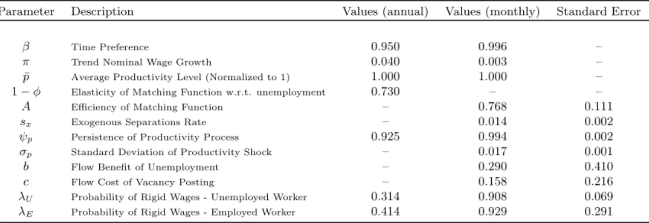
The theoretical model has 11 parameters: β, π, φ, A, ψp, σp, b, c, λE, λU,andsx. We set β to

5 percent annually, as in Shimer (2005) and Hall (2005). Our model does not explicitly feature real productivity growth, so we set π to 4 percent annually to capture both price inflation and productivity growth. Implicitly, β represents a discount factor that encompasses both pure time preference and trend growth in consumption.

We estimate eight of the nine remaining parameters, Θ ={A, ψp, σp, b, c, λE, λU, sx}, via indirect

inference, in order to match a set of simulated moments, ˆµs(Θ), to a set of real-world target moments

(33)

the resulting share of job surplus accruing to the worker (Hosios 1990).23 The estimated parameters are the values that minimize ˆΘ = arg min

Θ

[ˆµs_(Θ)₋_µ_]0_W−1_[ˆ_µs_(Θ)₋_µ_{], where the weighting function}

W is a diagonal matrix of the squares of the target moments.

Estimating the model via indirect inference helps to correct for potential sources of error in our empirical approach. The first is mis-classification of job stayers and job finders. The second is bias in our measurement of the fraction of counterfactual wage cuts prevented by downward nominal wage rigidity. Besides helping to correct for potential measurement error, the indirect inference procedure provides a tight link between the reduced form empirical estimates and their counterparts in the simulated data.

Table 1.5 displays the empirical moments that we target, along with the simulated moments that result from the estimated model. All moments were calculated over the years 1980 to 1997. The unemployment rate, u= .061, job-finding rate, f = .42, and median duration of unemployment,

D= 3.9 months, are targeted to CPS quarterly averages.24

The remainder of the target moments are derived from the PSID data.25 _{Wage rigidity for}

incumbent workers (wr_cs= 0.53 for job stayers) and new hires (wr_cf = 0.36 for job finders), outlined

in section 3 above, are derived from the PSID data for 1980-1997. The difference between the 50th and 80th percentile of annual real log wage changes, Φ80−Φ50, is estimated from the same

dataset to be about 11 percentage points. The moments ˆαand ˆσlnw, are taken from the regression

lnwit=δ0+δt+αlnwit−1+uit, and are estimated as ˆα= 0.88 and ˆσlnw= 0.19.

Although in principle all of the target moments can influence all of the estimated parameters, in practice some of the target moments have a larger influence on some parameters than on others. The Calvo parametersλE andλU are primarily determined by the wage rigidity target moments (λU is

also influenced by D). The parameters governing the productivity process, ψp andσp, are heavily

influenced by many of the targets, butψpis directly characterized by ˆα, whileσp is influenced more

by ˆσlnw and D. The matching efficiency parameterA and the exogenous separations rate sx are

jointly determined by uand f. The cost of vacancy creationc and the flow unemployment benefit

bare characterized in part by the share of job surplus accruing to the worker.

The model matches the target momentsu,f, ˆα, Φ80−Φ50, andD reasonably closely. ˆσlnwwas

more difficult to match, which is perhaps unsurprising given the model’s lack of heterogeneity in job amenities, investment in human capital, or match quality between jobs and workers. The estimated

23_{This condition ensures that the number of vacancies is efficient in an environment with flexible wages.} 24_{The first two are from data constructed by Robert Shimer using the CPS. For more details, see Shimer (2012).} 25_{We have also estimated this model using CPS-derived moments, with qualitatively similar results, but we highlight} the PSID data because it is a superior dataset for multi-year analysis of the evolution of wages (as opposed to a single one-year change for each worker in the CPS).

(34)

model matches the proportion of wage cuts prevented by wage rigidity for job finders wr_cf quite

closely, but produces an estimate for job stayerswr_csthat is lower than in the data.

Table 1.6 lists the estimated parameter values and their standard errors. The values forλE and

λU could not be determined to be different from each other at the 95th percent significance level, and

they correspond to a probability of experiencing rigid wages of greater than 90 percent per month. The exogenous separations rate sx corresponds to a little more than half of the total separations

implied by the stationary unemployment and finding rates. The elasticity of the matching function with respect to unemployed workers 1−φ is 0.73, reflecting the “take-it-or-leave-it” nature of the wage demands of workers in our model, which causes the majority of the match surplus to accrue to the workers. Nonetheless, because workers realize that they may be unable to cut their wage demands in the future, they moderate their wage demands in the present, leaving a non-trivial share of the match surplus to the firm.26 _{The flow benefit of unemployment,}_b_{, is estimated to be quite low}

at 0.29, or approximately 30% of the average wage, which helps to moderate their wage demands. We estimate the following equation on our simulated data using individual-specific productivity levels and wages:

∆ lnwijt=β0,j +β1,j∆ lnyijt+εijt, (1.19)

We divide workers into seven groups j: 1) all employed workers, 2) incumbent workers who were employed in the previous month, 3) incumbent workers who have had continuous employment for at least a year, 4) newly hired workers, 5) workers who were hired in the previous 3 months, 6) unemployed workers, and 7) unemployed workers plus new hires. For each individual in each group we record the most recent observed wage and productivity data in the event that they were not employed in the prior period (e.g. newly hired workers). We use reservation wages in place of actual wages for unemployed workers.

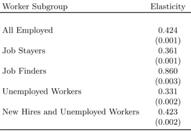
Table 1.7 shows the results of these regressions. Even with the high level of wage rigidity for job finders estimated in our model, the regressions show that their wages are very responsive to their productivity levels. The estimated elasticity of wages with respect to individual productivity is 0.86 for those who have been working for 3 months or less and 1.06 for new hires. Job stayers exhibit a much lower wage elasticity of 0.36. The reservation wages of unemployed workers exhibit a wage elasticity with respect to productivity of 0.33, much lower than for job finders, consistent with the survey data of Krueger and Mueller (2014). When we estimate the regression combining unemployed

26_{This result is reminiscent of Elsby (2009), who argues that firms will respond to downward nominal wage rigidity} by compressing wage increases in good times.

(35)

workers’ reservation wages with the observed wages of new hires, we estimate an elasticity of 0.42, similar to the elasticity for all employed workers. We interpret these results as supporting our contention that composition bias drives the apparent flexibility of the wages of new hires.

1.5.2 Dynamic Simulation

We use our estimated model to simulate a dynamic economy in which the aggregate productivity level changes. We run 1,000 simulations of the economy containing 10,000 workers over 14 years (168 months), discarding the first 10, and implement a permanent unanticipated productivity shock (with equal probability of a 1 percent increase or a 1 percent decrease) in the first month of year 12. The resulting simulated data represents 1,000 unique simulations of 12 months of base data and 36 months of data responding to the new permanent change in aggregate productivity. It is common knowledge among all agents in the model that the shock will be permanent.

To facilitate computation, we use policy functions of firms and workers that correspond to the eventual new steady state of the model immediately after the aggregate productivity shock hits. Although the model is not fully dynamic in that sense, we argue that it approximates the transition from one steady-state to another reasonably well for two reasons. First, following the logic of Shimer (2005) and Pissarides (2009), because the hiring and job separation probabilities are quite large in the model, the model will converge quickly to the new equilibrium after the aggregate shock.27

Additionally, employment relationships are on average long-lasting (46 months in the steady-state model). Thus, firms’ hiring and workers’ wage-posting decisions in the new steady state are likely to be a close proxy for their behavior in transition between states. We allow free entry of vacancies to adjust to period-specific labor market flows.

Figures 1.3 and 1.4 show the impulse-response functions of unemployment, job finding, separa-tions, wage demands, and productivity after positive and negative shocks to aggregate productivity. The unemployment rate behaves asymmetrically with regards to the productivity shocks, as a pos-itive productivity shock leads to a smaller change in unemployment and a larger initial change in wages than a negative productivity shock causes. This asymmetry results from wages being down-wardly rigid but updown-wardly flexible in our model.

Figure 1.3 also decomposes unemployment into its various sources in the model. Exogenous separations and rigidity-based separations are the proximate causes of a little less than half the total unemployment in any given period, while rigid wages for unemployed workers and failures to

27_{In the baseline steady state, the job finding probability is 0.395 and the separation probability is .022, implying} a half-life for the deviation of unemployment from its steady state value of approximately 1.66 months.

(36)

match with a vacancy account for the remainder. In the event of a negative shock, unemployment due to rigid wages for both the employed and the unemployed increases significantly, but after the initial period (during which many workers flow from the employed to unemployed states) the effect of rigidity for unemployed workers dominates the effect of rigidity for employed ones. Therefore, the finding rate has a slower adjustment process after a negative shock than the separation rate and contributes more overall to the volatility of unemployment, as seen in the bottom panels of figure 1.4.

The observed labor productivity of job finders also responds asymmetrically to positive and negative productivity shocks. Because idiosyncratic productivity evolves as a Markov process inde-pendent of firm and employee behavior, these changes are driven entirely by compositional changes. The new hiring spurred by a positive productivity shock brings more marginal employees into em-ployment, leading to a gradual rise in average observed productivity. The wage rigidity for entrants binds much more strongly for hires in the event of a negative shock than for a positive one, leading to the composition of new hires with flexible wages rising dramatically in recessions. Thus, a neg-ative shock leads to a rapid decline in average productivity among finders, from which it gradually recovers.

This pattern is also evident in the wage demands of job finders versus all workers, shown in the second row of figure 1.4. Real wages track the path of productivity closely, illustrating the importance of wage flexibility in achieving full employment in an economic downturn. In the model, unemployed workers, from whom the pool of new hires is selected, do not exhibit this kind of flexibility on average. The ratio of the reservation wage to the idiosyncratic productivity level of the unemployed, shown in the third row of figure 1.4, does not respond any more dramatically than the wage-to-productivity ratio of employed workers. The gap between these ratios constitutes a major barrier to unemployed workers’ chances of becoming re-employed.

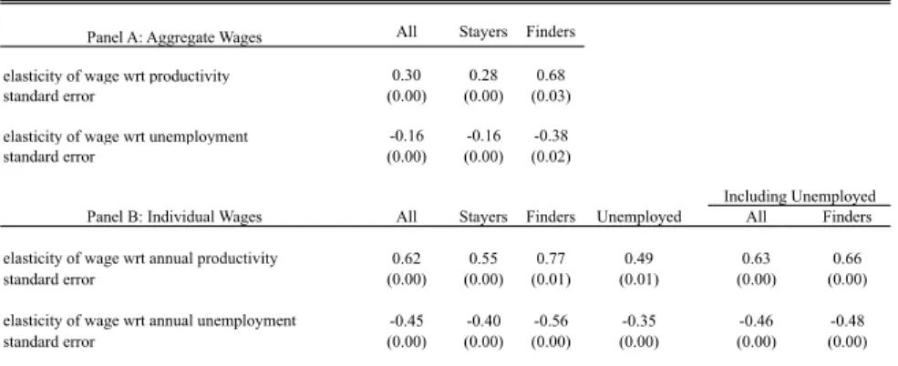
We use the dynamic responses of the model to the aggregate productivity shocks to estimate aggregate elasticities in the spirit of the empirical work in section 1.2. To measure the responsiveness of aggregate wages in various subgroups of workers (all workers, new hires, and incumbent workers), we randomly select a “survey month” from the quarter before the productivity shock and measure the log change in average wages three months later. The upper panel of table 1.8 displays the results of regressing these log changes in average wages on equivalent economy-wide changes in average labor productivity or the unemployment rate. The elasticity of average wages with respect to productivity is 0.68 for new hires (defined as workers who have found a job in the past three months), significantly higher than it is for the working population as a whole, 0.30. Both of these

(37)

elasticities compare closely with the elasticities found in Haefke et al. (2013). A similar pattern holds for the elasticities of average wages with respect to the unemployment rate, as all workers exhibit an elasticity of -0.16, versus -0.38 for job finders.

The bottom panel of table 1.8 demonstrates the effect of aggregate productivity and the un-employment rate on individual wage changes by worker category. In this analysis a job finder is defined as in the PSID data to be a worker who was unemployed or out of the labor force at any point between surveys (typically 12 months). Job finders appear to be more responsive to changes in labor market conditions, as indicated by the greater responsiveness of their wages to labor market conditions. Including unemployed workers with job finders, as in the rightmost column, indicates that part of that finding stems from composition bias. Workers who remain unemployed actually exhibit more rigid wages, as measured by less elastic wage demands with respect to labor market conditions, than workers who have maintained a job over the course of a year. This result again stems from the negative selection with regard to wage flexibility associated with unemployed workers in the model: unemployed workers are much more likely to have experienced rigid wages than the working population.

1.6 Conclusion

This paper has demonstrated that composition bias potentially accounts for the apparent flex-ibility of the wages of newly hired workers. Newly hired workers are disproportionately likely to have flexible wages relative to the pool of unemployed workers. Empirical analyses that omit the reservation wages of the unemployed are prone to over-estimate the responsiveness of potential new hires to macroeconomic conditions. Of course, because reservation wages are not regularly measured in most economic datasets, this problem is inherently difficult to solve.

Using a model that explicitly ascribes high degrees of nominal wage rigidity to both incum-bent workers and new hires, we are able to reconcile the dissonant statistics in the empirical data. Furthermore, when we re-estimate the key empirical elasticities including the reservation wages of unemployed workers along with the observed wages of new hires, the combined wages are noticeably less responsive to labor market conditions.

Dynamic simulations point to the same conclusion. The simulated elasticities of wages with respect to productivity closely match those in the U.S. data. A negative productivity shock leads to a persistent increase in unemployment attributable to wage rigidity among the unemployed, but the aggregate wages of new hires appear flexible because of selection effects. Therefore, we argue