Analyzing the Impact of Trade Reforms
on Welfare and Income Distribution Using
CGE Framework: the Case of the Philippines
*CAESAR B. CORORATON
*** This paper was funded by the East Asian Development Network (EADN). ** Senior Research Fellow, Philippine Institute for Development Studies
Number 57, First Semester 2004, Volume XXXI, No. 1
T
rade liberalization was one of the major economic reform programs implemented in the last 15 years. The program was pursued in various phases incorporating policies of tariff reduction, simplification of tariff structure and “tariffication” of quantitative restrictions. Some of these reforms were pursued unilaterally, while others were done under various multilat-eral agreements such as the World Trade Organization (WTO), as well as regional agreements among members of the Association of Southeast Asian Nations (ASEAN) such as the ASEAN Free Trade Area (AFTA).Trade liberalization—particularly tariff reduction, which is the focus of the paper—triggers changes in both sectoral price ratios and domestic-foreign price ratios. These changes in turn cause a reallocation in production and resources, which lead to a contraction in some production sectors and an expansion in others. Furthermore, it generates a web of direct and indirect changes that makes it ex-tremely difficult to track down the effects on various households. Gaining a better understanding of the effects may therefore require an economy-wide model. One such model is the computable general equilibrium (CGE). The objective of the paper is to construct a CGE model calibrated to Philippine data and simulate the impact of tariff reforms on income distribution and welfare.
In a CGE framework, the effects of tariff reform on households may be traced through two channels: income and consumption channels. In the income channel, tariff reform may generate a series of changes in sectoral imports, ex-ports, production, demand for factors and factor payments and ultimately,
house-hold income. Househouse-holds endowed with factors that are used intensively in the expanding sectors may benefit from the tariff reform. On the other hand, in the consumption channel, tariff reform may change the structure of consumer prices. It will benefit those household groups whose consumer basket is dominated by goods with declining prices as a result of the tariff reform. Through these two channels, this paper will attempt to trace the effects of the reduction in tariff rates from 1994 to 2000 on household income and welfare.
A QUICK LOOK AT LITERATURE
Cloutier et al. (2002) provide a comprehensive review of the CGE literature, fo-cusing on the analysis of welfare, poverty, and distributional effects of trade liber-alization. Two general findings may be highlighted:
While the literature has applied various model specifications in trade reforms, the results are analyzed using two broad transmission mecha-nisms: income and consumption mechanisms. On the income side, trade reform impacts on imports, production, factor remuneration, and ulti-mately, household income. On the consumption side, trade reform im-pacts on the macroeconomy, altering as a result the structure of con-sumer prices.
While there are broad similarities in the overall specification of CGE models, the effects of trade reform are generally country-specific. The results greatly depend upon the countries’ initial conditions in the struc-ture of their foreign trade, production and factors, consumption and sources of household income. The results also depend on the degree of factor substitution in production and on commodity substitution in the consumer basket. Furthermore, the overall results depend upon the extent of the reform in terms of the magnitude of the reduction in trade barriers.
A lesson here is that one cannot make a general statement on the effects of trade reforms because the results are country-specific. Trade liberalization de-pends upon the structure of the economy and the extent of the reform. Therefore, it is extremely important to take into account the structure of the economy when analyzing the possible impacts of trade liberalization. It is necessary to go through the tedious task of constructing a social accounting matrix (SAM) that is based on actual data and to specify a CGE model that is based on the SAM.
Cororaton (1994) provides a comprehensive review of literature on CGE modeling in the Philippines. He observes that, while there are a number of CGE models available in the country with various sectoral breakdowns, most focus on
analyzing production efficiency and reallocation effects. Analyses of the impacts of trade reforms on households are either not emphasized or, worse, completely omitted.
An exception is Cororaton (2000), which attempts to analyze the effects of tariff reform on household welfare. Unfortunately, the paper suffers from two weak-nesses: (1) The simulation was based on a CGE model that was calibrated in 1990, making it a bit outdated given that much of the tariff reforms took place in the mid-1990s. (2) Households were disaggregated in income deciles, making it con-ceptually difficult to pin down the household effects of a policy shock since the decile category of households can also change as a result. A better strategy would have been to characterize households by resource endowments (e.g., educational attainment), because the extent of reclassification after a policy change, if at all, would have been much less.
These two weaknesses are addressed in this paper. First, a CGE model is specified and calibrated using a 1994 SAM that was constructed from the 1994 Input-Output Table, the 1994 Family Income and Expenditure Survey, and various 1994 official economic information. Second, the household sector is disaggre-gated by socioeconomic groupings that are based on the educational attainments of household heads. More specifically, households are classified into urban and rural classes and then by the educational category of their household heads.
TRADE REFORMS
The trade reform program has three major components: the 1981-1985 Tariff Re-form Program (TRP); the Import Liberalization Program (ILP); and the compli-mentary realignment of the indirect taxes. In TRP, there was a narrowing of the tariff rate structure from a range of 0-100 percent to 10–50 percent. During the period 1983-1985 sales taxes on imports and locally produced goods were equal-ized. Also, the mark-up applied on the value of imports (for sales tax valuation) was reduced and eventually eliminated.
However, because of balance of payments issues and the economic and political crises of the mid-1980s, the import liberalization program was suspended. Indeed, some of the items that were deregulated earlier were re-regulated during this period. Only when the Aquino government took over in 1986 was the trade reform program resumed. This had the effect of reducing the number of regulated items from 1,802 in 1985 to 609 in 1988. In addition, export taxes on all products except logs were abolished as well.
In 1991, the government launched the TRP-II, with the issuance of Executive Order (EO) 470. An extension of the previous program, it sought to realign tariff rates over a five-year period, by narrowing the range of the rates through a series
of reductions in the number of commodity lines with high tariffs and by expanding the number of commodity lines with low tariffs. In particular, the program was intended to cluster tariff rates within the 10–30 percent bracket by 1995. By the end of the program in 1995, however, only about 10 percent of the total number of commodity lines had a 0-5 percent tariff rate; still, others were subject to a 50 percent tariff rate.
“Tariffication” of quantitative restrictions (QRs)—i.e., converting QRs into tariff equivalent—started in 1992 with the implementation of EO 8. There were 153 commodities whose QRs were converted into tariff equivalent rates. In a num-ber of cases, tariff rate hike were over 100 percent, especially during the initial years of the conversion. However, a built-in program for the phase-down of the tariff rates over a five-year period was also put into effect. Furthermore, in the same executive order, tariff rates on 48 commodities were further realigned.
Deregulation continued on the next 286 items under the tariffication pro-gram. By the end of 1992, only 164 commodities were covered under the QRs. However, Memorandum Order 95 in 1993 reversed the deregulation process. In fact, QRs were reimposed on 93 items, bringing up the number of regulated items under the QR to 257. This re-regulation came largely as a result of the Magna Carta for Small Farmers in 1991.
Major reforms were implemented under the TRP-III. The program was em-bodied in the following executive orders: (1) EO 189, implemented on January 1, 1994, provided reduced tariff rates on capital equipment and machinery; (2) EO 204 on September 30, 1994 mandated tariff reductions in textiles, garments and chemical inputs; (3) EO 264 on July 22, 1995 reduced tariffs on 4,142 harmo-nized lines in the manufacturing sector; and (4) EO 288 on January 1, 1996 re-duced tariffs on “nonsensitive” components of the agricultural sector. The restruc-turing of tariff under these various executive orders involved a reduction in both the number of tariff tiers and the maximum tariff rates. In particular, the program established a four-tier tariff schedule, namely: three percent for raw materials and capital equipment that are not available locally; 10 percent for raw materials and capital equipment that are available from local sources; 20 percent for intermedi-ate goods; and 30 percent for finished goods.
Another major component of the tariff program is the uniform tariff rate, which was scheduled for implementation starting 2004. Policy discussions on the issue, however, are still ongoing. Determining the level of tariff rate to be imple-mented uniformly across sectors remains an unsettled issue.
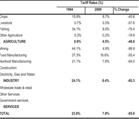
Table 1 shows the weighted average tariff rates in 1994 and 2000 across various sectors. The overall weighted tariff rate declined over these years by -65 percent: from 23.9 percent in 1994 to 7.9 percent in 2000. The decline in the industry
tariff rate was much higher than in agriculture: -65.3 percent and -48.8 percent, respectively.
In terms of specific sectors, the largest drop in tariff rates was in mining (-88.9%), while the lowest decline was in other agriculture (-19.9%). In terms of tariff rate level in 2000, food manufacturing still had the highest rate of 16.6 per-cent. Other agriculture had the lowest tariff rate of 0.2 perper-cent. These changes in tariff rates over the period were the ones utilized in the simulation experiment.
TARIFF REFORM AND GOVERNMENT REVENUE
Revenue from import tariff is one of the major sources of government funds. Table 2 shows the structure of the government’s sources of revenue. In 1990, the share of revenue from import duties and taxes to the total revenue was 26.4 percent. This increased marginally to 27.7 percent in 1995. However, the share dropped significantly to 17.1 percent in 2001. One of the major factors behind the decline was the tariff reduction program.
The share of direct taxes (income and profit direct taxes combined) increased consistently from 27.3 percent in 1990 to 30.7 percent in 1995 and to 39.6 percent
in 2001. On the other hand, the share of government revenue from excise and sales taxes dropped from 27.2 percent share in 1990 to 23.4 percent in 1995. It, however, recovered to 29.3 percent in 2001.
Since tariff revenue is a major source of government funds, a tariff reduc-tion program could therefore have substantial government budget implicareduc-tions especially if it is not accompanied by another compensatory tax financing scheme. In fact, it could pose a major policy challenge especially in a situation where the government’s budget deficit is growing.
The last three years saw a widening government budget deficit. From a bud-get surplus of 0.6 percent of gross national product (GNP) in 1995, the budbud-get balance flipped to a deficit of -3.6 percent in 1999 and another -3.8 percent in 2000. In 2001, the deficit was still at -3.8 percent of the GNP. This persistent government imbalance, if remained unchecked, could not only create a host of undesirable macroeconomic effects but also put into question the viability of a continued implementation of the tariff reduction program unless other compensatory tax financing measures such as income tax and other excise and indirect taxes, are implemented.
THE STRUCTURE OF THE ECONOMY IN THE 1994 SAM
The impact of tariff reduction depends upon the initial conditions of the economy in the base year (which is 1994 in the present context) in terms of the structure of foreign trade (imports and exports), production, household consumption, factor endowments and sources of income. A brief discussion on these is given in this section. The discussion is based on the data in the constructed 1994 SAM.1 1 Appendix C discusses how the SAM was constructed and contains sources of information. Table 2. Sources of national government revenue (%)
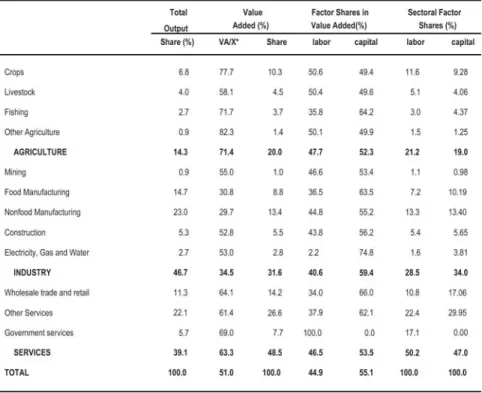
Table 3 shows the structure of production. Industry contributes 46.7 per-cent to the overall gross value of economic output. Of the total contribution of industry, 23 percent comes from the nonfood manufacturing sector and another 14.7 percent from the food manufacturing. The output contribution of the entire service sector is 39.1 percent, of which 22.1 percent comes from other services and 11.3 percent from wholesale and retail trade. Total agriculture contributes 14.3 percent to the total, of which 6.8 percent comes from crops and another four per-cent from livestock.
Agriculture and service sectors have high added content. The value-added shares to their respective total value of output are 71.4 percent and 63.3 percent, respectively. Industry has a far smaller value-added ratio of 34.5 percent. Within industry, manufacturing has the smallest value-added ratio: 30.8 percent for food manufacturing and 29.7 for nonfood manufacturing. Nonfood manufac-turing has the lowest ratio among all sectors.
In terms of sectoral contribution to the overall value added, the service sector contributes the largest share of 48.5 percent, followed by the industry sector (31.6%). Of the total industry share, nonfood manufacturing contributes 13.8 percent.
About 55.1 percent of the overall value added is payment to capital, while the remaining 44.9 percent is payment to labor. Agriculture has the highest labor payment of 47.7 percent, while industry has 40.6 percent.
Table 4 shows the structure of sectoral exports and imports (which include both merchandise and nonmerchandise trade) in the SAM. In the import side, industry, particularly the nonfood manufacturing sector, dominates. Total industry has 88.8 percent of total imports, of which 76.1 percent comes from nonfood manufacturing. A similar structure applies to the export side, with industry captur-ing almost 60 percent. Of the total industry export share, 48.2 percent is from nonfood manufacturing exports.
The dominance of industry, particularly the nonfood manufacturing sector, in the country’s foreign trade is largely due to the phenomenal rise of the semi-conductor sector in the 1990s. This is seen in Table 5 where the breakdown of merchandise export is presented. The export share of electrical and electrical
ment, which is largely dominated by exports of semiconductor, surged from 24 percent in 1990 to 59.5 percent in 2000.
Garments used to be a major export item of the country before the 1990s. However, its share dropped significantly in the last decade from 21.7 percent in 1990 to only 6.9 percent in 2000. The same declining trend is observed in agricul-ture-based exports over the same period. In 1990, agriculagricul-ture-based exports had a combined share of 18.2 percent. Over the years, it dropped consistently to reach 4.6 percent only in 2000.
Activities in the country’s semiconductor industry have extremely small value-added contribution. This is because the sector as a whole is dominated by assembly type operations only. Almost all of its input requirements are imported. Practically, labor is the only local contribution. Furthermore, the sector has a very small link with the rest of the economy because semiconductor firms are usually located in special places such as the export processing zones. Thus, while the share of the sector to the total value of output is large, its contribution to the total value added is small.
Before discussing the structure of consumption and the sources of income of households, it would be necessary to have an idea of the disaggregation of the Table 5. Merchandise exports (US $million, %)
Coconut products 503 989 595 6.1 5.7 1.6 Sugar and products 133 74 57 1.6 0.4 0.2 Fruits and vegetables 326 458 528 4.0 2.6 1.4 Other agrobased products 431 575 486 5.3 3.3 1.3 Forest products 94 38 44 1.1 0.2 0.1 Agriculture based 1487 2134 1710 18.2 12.2 4.6 Mineral products 723 893 650 8.8 5.1 1.7 Petroleum products 155 171 436 1.9 1.0 1.2 Manufactures 5707 13868 33989 69.7 79.5 91.2 Electrical
and electrical equip’t 1964 7413 22178 24.0 42.5 59.5 Garments 1776 2570 2563 21.7 14.7 6.9 Textile yarns/fabrics 93 208 249 1.1 1.2 0.7 Others 1874 3677 8999 22.9 21.1 24.1 Other exports 114 381 502 1.4 2.2 1.3
Industry based 6699 15313 35577 81.8 87.8 95.4
Total merchandise exports 8186 17447 37287 100.0 100.0 100.0
Value Shares (%)
1990 1995 2000 1990 1995 2000
household sector. Table 6 shows the definition of the household sector. There are 12 household groups in the analysis (six urban household groups and another six rural). The disaggregation is based on the type of work and the educational attain-ment of the household heads.
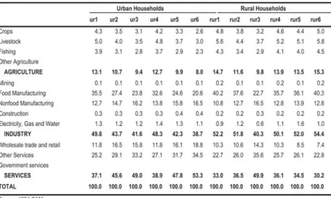
The consumption structure of each household group is presented in Table 7. The largest items in the consumer basket across household groups come from food manufacturing, service and nonfood manufacturing sectors. Across house-hold groups, however, the consumption ratios vary considerably. For example, 35.5 percent of Ur1’s consumption basket comes from food manufacturing. For Ur2, it is only 27.4 percent. Thus, given these differences in the structure of con-sumption basket across household groups, a change in the structure of consumer prices as a result of a tariff reduction will have differentiated effects across groups. Table 8 presents the structure of households’ sources of income. Four types of labor are considered in the analysis: there are two types of agriculture labor and two types of production labor, each categorized as skilled and unskilled. Skilled production workers include professionals, managerial and other related workers. Skilled worker is defined as one with at least a high school diploma. The rest are categorized as unskilled.
There are four sources of capital income: income from capital used in agri-culture, in industry, in wholesale and retail, and in other services. Capital income is separated from various sectors because in the model specification, sectoral capital is fixed. The zero-profit condition that is required in the CGE model is imple-Table 6: Household definition
Table 7 : Household consumption share (%)
Table 8: Sources of household income
Urban households Rural households
ur1 ur2 ur3 ur4 ur5 ur6 rur1 rur2 rur3 rur4 rur5 rur6
Agriculture-skilled 0.0 1.0 0.2 0.0 0.1 0.1 0.0 82.1 0.7 0.0 11.2 0.1 Agriculture-unskilled 6.6 0.0 0.1 1.4 0.0 0.1 64.5 0.0 25.6 16.2 0.0 13.2 Production-skilled 0.0 88.0 83.4 0.0 48.8 14.1 0.0 2.8 5.0 0.0 3.5 0.1 Production-unskilled 64.0 0.0 2.3 24.7 0.0 2.3 3.6 0.0 1.4 0.7 0.0 0.8 Capital in agriculture 1.4 0.4 0.4 8.7 2.1 2.6 5.3 0.3 4.4 19.1 20.0 26.8 Capital in industry 7.8 1.0 1.7 19.3 9.4 45.6 2.7 0.4 0.7 18.0 0.1 11.3 Capital in WRT* 4.6 1.2 2.5 12.3 10.9 10.3 0.7 2.6 0.4 6.1 0.1 5.58 Capital OSER** 8.6 3.6 3.8 14.2 10.5 7.0 9.2 8.1 21.3 18.0 13.7 17.3 Dividends 1.6 3.3 3.4 8.3 8.1 15.6 0.3 0.0 0.5 2.4 33.6 7.4 Government transfers 2.9 0.5 0.5 4.7 3.2 1.0 13.3 2.6 37.6 15.8 14.1 16.2 Foreign sources 2.5 1.2 1.8 6.5 6.9 1.3 0.5 0.6 2.4 3.7 3.7 1.1 100.0 100.0 100.0 100.0 100.0 100.0 100.0 100.0 100.0 100.0 100.0 100.0
WRT whiolesale and retail trade OSER other services
mented through a market-clearing rate-of-return to capital per sector. Thus, a policy shock will find its way, among others, through changes in the rate-of-return to capital per sector. A differentiated sectoral rates-of-return to capital will, in turn, result in differentiated capital income from various sectors.
Other sources of household income include dividends, government trans-fers, and foreign income. In the case of the Philippines, foreign income is largely from foreign remittances of contract workers.
One can observe that there are large differences in the sources of income across household groups. Tariff reduction that affects relative price ratios will affect factor demand, which in turn will affect factor prices (both wages and the rate-of-return to capital). These changes will have differentiated effects on house-hold income.
THE CGE MODEL
A CGE model was specified and calibrated to the 1994 SAM to analyze the ef-fects of tariff reforms on income distribution and welfare. The model is called PCGEM, whose complete set of equations is presented in the appendix.
PCGEM has 12 production sectors, of which four comprise agriculture, fish-ing and forestry. There are five sectors in industry, includfish-ing utilities and con-struction. Service is composed of three sectors, including government service sec-tor. The model distinguishes two factor inputs (i.e., labor and capital) to deter-mine sectoral value added using CES production function. The model incorpo-rates four types of labor: skilled agriculture labor, unskilled agriculture labor, skilled production labor and unskilled production labor. Agriculture labor is devoted to the agriculture sector only. Similarly, production labor works in the nonagriculture sector only. As defined earlier, skilled production workers include professionals, managerial and other related workers with at least a high school diploma.
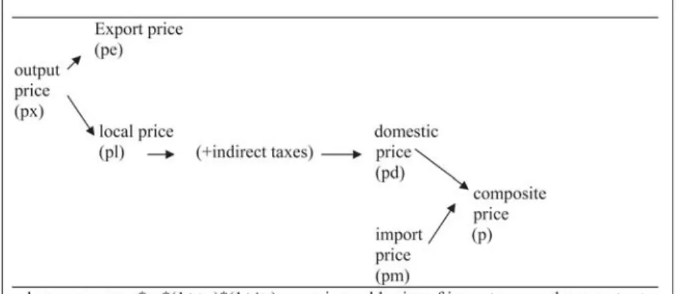
Sectoral capital, however, is fixed. Value added (together with sectoral in-termediate input, which is revealed using fixed coefficients) determine total out-put per sector. In both product and factor market, prices adjust to clear all markets. Figure 1 shows the basic price relationships in the model. Output price px affects export price pe and local prices pl. Indirect taxes are added to the local price to determine domestic prices pd, which together with import price pm, will deter-mine the composite price p. The composite price is the price paid by the consumers. Import price pm is in the domestic currency, which is affected by the world price of imports (pwm), exchange rate (er), tariff rate (tm) and indirect tax rate (itx). Therefore, the direct effect of tariff reduction is to reduce pm. If the reduc-tion in pm is significant enough, the composite price p will also decline. Note that consumers in the market face the composite price. Thus, the composite price is also the consumer price.
Consumer demand is based on the Cobb-Douglas utility functions. Armington-constant elasticity substitution (CES) function is assumed between local and imported goods, while a constant elasticity of transformation (CET) is imposed between exports and local sales. Production and trade elasticities are discussed and presented in the appendix.
The model closure used has the following features:
✦ Government account closure. Government consumption is held fixed. Government income is also fixed by introducing an automatic com-pensatory tax. There are three comcom-pensatory taxes that are separately part of an experiment in this paper: income tax, indirect tax, and a combination of indirect and income tax. These two assumptions to-gether effectively fix government savings.
✦ Current account closure. The current account balance is fixed. This in effect avoids the possibility of foreign financing for the tariff reduc-tion program. That is, foreign debt is not accumulated while the re-form process is undertaken. Moreover, the nominal exchange rate is fixed as well. What clears the current account balance is the movement in the real exchange rate, which is captured effectively by the changes in the ratio between domestic and foreign prices.
✦ Total investment closure. Total savings is composed of government savings, foreign savings (both of which are fixed) and private savings. The experiments conducted in the paper all assume a neo-classical closure wherein total savings is invested.
EXPERIMENTS
There are four experiments conducted in this study. Below is a brief description of each.
Experiment 1 (E1). This experiment involves simulating the actual reduc-tion in sectoral tariff rate as shown in Table 1. The compensatory tax is through additional income tax. This experiment is in line with the structure of the govern-ment revenue as presented in Table 2, where an increasing share of income tax revenue is observed during the period of declining share of tariff revenue. In ef-fect, this experiment is revenue-neutral as it reduces the distortion coming from tariff rates. The results of this experiment are discussed in great detail below.
Experiment 2 (E2). This experiment is the same as E1 except that the com-pensatory tax is through additional indirect tax on output. Although this experi-ment is revenue-neutral, the additional indirect tax in effect replaces the distortion coming from tariff rates with distortion from indirect output tax. The term distortion in the present context implies that the imposition of taxes results in changes in the sectoral price ratios. The results of this experiment are presented in the appendix.
Experiment 3 (E3). This experiment is the same as in the previous two ex-periments except that the compensatory tax is through a combination of additional income and indirect taxes. The results are also presented in the appendix.
Experiment 4 (E4). This experiment involves a set of simulation runs testing the sensitivity of the distribution and welfare effects to changes in production and trade elasticities. The Armington and the CET elasticities in trade and the substi-tution parameters in production were adjusted by +20 percent and -20 percent from the base values. The results are presented in the appendix.
SIMULATION RESULTS
From tariff reduction to reallocation of production
The price and volume effects of experiment E1 are presented in Table 9. Tariff reduction results in an overall reduction in the domestic price of imports (δpm) of -10.4 percent. Similarly, the overall composite price (δpq) declines by -4.1 percent while the domestic prices of local goods (δpd) declines by -3.4 percent. Thus tariff reduction translates into reduced domestic prices.
What are the volume effects? The reduction in tariff results in shifts in the relative import-domestic price ratios, which in turn trigger substitution between imports and domestically produced goods. For example, import volume (δm) in-creases by 6.3 percent while domestic production declines by -0.6 percent. Taken together, these changes result in a marginal increase in the total goods available in the market as shown by a 0.6 percent improvement in the composite goods (δq).
The overall decline in domestic prices creates an effective real exchange depreciation, which in turn increases export competitiveness across almost all
sectors. This is reflected in the reduction in the sectoral price ratio between export prices and the corresponding local prices δ(pei/pli), where pei is the export price in domestic currency and pli is local prices without indirect taxes. There is a marginal increase of 0.3 percent in the ratio for other agriculture but this sector has very small export share (thus, its impact on the overall export is correspondingly very small, too). Because of these effects, overall export increases by 6.1 percent, which in turn increases total output marginally by 0.6 percent.
On the whole, tariff reduction results in an increase in: (1) imports because of lower import prices; (2) exports because of improvement in competitiveness due to lower domestic prices; (3) overall output because of the export pull; and (4) total goods available in the market because of higher imports. However, domestic production for domestic sales (δd) declines because of substitution effects.
What are the effects at the sectoral level? The effects vary considerably across sectors, triggering reallocation of output. The effects are largely due to the Table 9. Price and volume effects (E1)
Price changes (%) Volume changes (%)
dpmi dpdi dpqi dpxi d(pe/pl)i dmi dei ddi dqi dxi Crops -5.9 -0.9 -1.0 -0.8 -0.9 8.4 -0.8 -2.0 -1.8 -1.9 Livestock -0.4 -1.1 -1.1 -1.1 -1.1 -2.9 -1.4 -1.9 -1.9 -1.9 Fishing -18.5 -1.9 -2.0 -1.5 -1.9 20.3 1.0 -1.9 -1.8 -1.3 Other agriculture -0.1 0.4 0.3 0.3 0.3 0.5 0.1 0.1 0.1 AGRICULTURE -3.4 -1.1 -1.1 -0.9 3.3 0.1 -1.8 -1.7 -1.6 Mining -25.8 -8.1 -21.5 -4.5 -8.0 12.4 0.7 -11.3 5.6 -6.0 Food manufacturing -14.0 -2.0 -3.0 -1.8 -2.0 12.7 0.3 -2.1 -1.0 -1.9 Nonfood manufacturing -10.4 -6.5 -8.5 -4.2 -6.5 6.3 12.1 2.2 4.2 5.7 Construction 0.0 -2.0 -2.0 -2.0 -2.0 -1.4 3.6 1.1 1.0 1.1
Electricity, gas and water 0.0 -2.4 -2.4 -2.4 -2.4 3.1 0.1 0.1 0.2
INDUSTRY -11.9 -3.9 -6.6 -3.1 7.2 9.9 0.1 2.4 2.3
Wholesale trade and retail 0.0 -1.1 -1.1 -0.9 -1.7 0.2 -1.1 -1.1 -0.8
Other services 0.0 -1.7 -1.6 -1.5 -3.2 0.9 -1.1 -1.3 -0.8
Government services -0.4 -0.8
SERVICES 0.0 -1.5 -1.4 -1.2 -3.2 0.6 -1.1 -1.2 -0.7
TOTAL -10.4 -3.2 -4.1 -2.0 6.3 6.1 -0.6 0.6 0.6
where
mi imports pmi import (local) prices ei exports pei export (local) prices di domestic sales pdi domestic prices qi composite commodity pli local prices xi total output pxi output prices
differences in the sectoral structure of imports and exports, initial tariff rates, and the trade elasticities. As discussed below, the differentiated sectoral results, espe-cially on factor prices, contribute largely to the varied effects across household groups.
Industry as a whole realizes the largest drop in import prices (-11.9%) as compared to agriculture’s import prices drop of -3.4 percent. Among specific sec-tors, the largest drop in import prices is observed in mining (-25.8%), in food manufacturing (-14.0%), and in nonfood manufacturing (-10.4%). These differen-tiated outcomes are effects of the different levels of initial tariff rate.
The sectoral effects on import volume are due to the differentiated effects on import prices and on the differences in the import elasticities (the Armington elasticities). Taking these factors together results in the largest increase in import volume (δmi) in fishing (20.3%), in food manufacturing (12.7%) and in crops (8.4%). Import volume for the nonfood manufacturing sector registers an increase of 6.3 percent only. However, since the nonfood manufacturing sector is the largest importer (76.1% of total imports in Table 4), the bulk of the increase in the overall import volume comes largely from this sector.
One set of findings on nonfood manufacturing needs further elaboration. In particular, attention should be directed to the results on its imports (δm), domestic production (δd) and the composite (δq), since nonfood manufacturing is a major contributor to the various totals. One may observe that the drop in its import prices is larger than the decline in its domestic prices (-10.4% and -6.5%, respectively). Thus, one would expect that this relative price change favoring imports would lead to a reduction in domestic production. However, the result on domestic pro-duction indicates an increase of +2.2 percent. There are no inconsistencies in the results because the composite good (δq) for the sector registers an increase of 4.2 percent.2
Except for livestock, all sectors register an increase in exports. The increase is largely attributed to the improvement in export competitiveness across sectors. Recall that the export competitiveness is indicated by the decline in the price ratio
δ(pei/pli), where pei is the export price in domestic currency and pli is local prices without indirect taxes. One may observe from the results that the largest increase in export competitiveness is in mining (-8.0%) and in nonfood manufacturing (-6.5%). However, results on the mining sector may be less interesting because its share to the total export is small while that on the nonfood manufacturing are critical as this sector contribute largely to the overall exports of the country (48.2%
2 If one puts these results in the framework of production theory, where imports and domestic production are factor inputs and one isoquant indicates one level of output, the results would indicate an outward shift in the isoquant since q is higher together with higher imports and domestic production.
to total exports in Table 4). This outcome, together with the increase in domestic production for nonmanufacturing, brings about an overall increase in its total pro-duction of 5.7 percent. This is the only sector that registers a relatively significant increase in output.
Marginal increases are observed in the following sectors: other agriculture (+0.1%), utilities3 (+0.2%), construction (1.1%) and government services (0.4%).
Thus, the results indicate clearly that given the structure of the economy and the extent of the actual reduction in tariff rate, reallocation of production favors the nonfood manufacturing sector.
From reallocation of production to factor markets
What happens to the flow of resources across sectors? Since all sectoral capital is fixed, the flow of resources pertains to the sectoral movements of labor only across sectors as tariff is reduced. The results on factor price ratios and capital-labor ratios are important in assessing sectoral labor movements. The results are pre-sented in Table 10.
Table 10. Effects on factor
Crops 0.98 1.02 -1.3 -3.7 -0.4 -0.3 Livestock 0.99 1.02 -1.3 -3.7 -0.4 -0.3 Fishing 1.79 1.86 -1.2 -3.5 -0.1 -0.1 Other agriculture 1.00 0.99 1.3 0.3 3.6 3.7 AGRICULTURE -1.1 -3.4 Mining 1.15 1.31 -7.5 -12.6 -12.8 -15.3 Food manufacturing 1.74 1.83 -7.5 -12.6 -5.4 -8.0 Nonfood manufacturing 1.23 1.09 9.8 13.1 12.6 9.5 Construction 1.28 1.25 2.9 2.5 2.1 -0.7 Electricity, gas and water 2.97 2.95 1.6 0.6 0.2 -2.5
INDUSTRY 3.6 4.9
Wholesale trade and retail 1.95 1.99 -0.4 -2.3 -2.7 -5.4 Other services 1.64 1.68 -0.3 -2.2 -2.6 -5.3 Government services 0.4 -0.1 0.0 SERVICES -0.4 -1.4
TOTAL 0.9
Average wage 1.2 -2.2 -2.3 1.6 4.5 * L1, L2, L3 and L4 = labor type 1, 2, 3, and 4
Factor intensity Change Change (%) in labor demand (k/l)i in return Aggregate
base experi- to capital labor L1* L2* L3* L4* ment
Lower tariff leads to an increase in both the overall average rate-of-return to capital (0.9%) and the average wage rate of aggregate labor (1.2%). Across sec-tors, however, the results vary. For example, in the sectoral rate-of-return to capi-tal, three sectors indicate an increase: nonfood manufacturing (9.8%), construc-tion (2.9%) and utilities (1.6%). The rest show a decline. Thus, these changes trigger factor substitution in favor of labor as indicated by the decline in their capital-output ratios. It is interesting to note that in terms of labor, there is a ten-dency for the demand for skilled labor to be pulled up. For example, the demand for labor is higher for L3 (i.e., skilled production workers) than for L4 in the case of the nonfood manufacturing sector. In the case of both construction and utili-ties, the demand for L3 increases whereas the demand for L4 declines.
In sum, the experiment’s findings indicate that the nonmanufacturing sector benefits from both the effects of output reallocation and labor movement. Further-more, there are indications that, as a result of the shifts in both output and factor price ratios, factor substitution favors skilled production workers in nonfood manu-facturing, construction and utilities sectors. Also, agricultural wages decline while production wages improve. All these will have important implications on income of households as discussed in the next section.
From factor markets to household income
What are the effects on the sources of income of households? The results are presented in Table 11.
The results concerning the demand for labor indicate that in the case of agriculture there is a movement toward other agriculture sector. On the other hand, in the case of nonagriculture there is movement toward nonfood manufacturing, construction and utilities. Movement toward nonfood manufacturing, however, is significant at 13.1 percent.
Results on the average wage rate across labor types are particularly relevant in assessing the effects of household income. The effects indicate that agricultural wages decline for both skilled and unskilled, while production wages increase for both labor types. The decline in agricultural wages is largely due to the overall decline in the demand for labor in agriculture,4 which in turn is due to the decline
in the overall agriculture output. Since the supply of agriculture labor is fixed, any decline in factor demand due to lower output will lead to a lower wage rate. Wage rate is market-clearing in the model.
Meanwhile, wage rates for both skilled and unskilled production workers increase, but such hike is larger in the latter than in the former labor type. Again,
a similar mechanism is in effect. The supply of production labor is fixed. There-fore, the improvement in the demand for labor, which largely comes from the nonfood manufacturing sector because of the improvement in its output, trans-lates into higher wages for production workers.
Overall household labor income increases by 1.2 percent because of the tariff reduction. However, the increase favors urban over rural households. In fact, all urban households enjoy positive increase in labor income while all rural house-holds suffer from lower income. There is a decline in agricultural wages as com-pared to the increase in production wages as a result of tariff reduction. These differentiated effects on wages are in turn the effects of the reallocation of produc-tion that favor industry.
There are interesting results within urban households. The highest increase is observed in Ur4 (4.0%) and in Ur1 (3.8%). One should note that these groups have household heads who are unskilled workers. Again, the differentiated effects within urban households are due to the much higher increase in wages for un-skilled production workers (4.5% in Table 10) relative to the wages of un-skilled production workers (1.6%). rOne should note also that, as observed earlier, the differentiated effects in production wages offset the increase in demand for skilled production workers due to the tariff reduction.
Table 11. Effects on household income, percent change from base (E1)
Urban households Rural households
Total ur1 ur2 ur3 ur4 ur5 ur6 rur1 rur2 rur3 rur4 rur5 rur6
LABOR 1.2 3.8 1.5 1.7 4.1 1.6 1.9 -1.9 -2.1 -1.4 -2.0 -1.3 -1.8 L1 -2.2 0.0 -2.2 -2.2 0.0 -2.2 -2.2 0.0 -2.2 -2.2 0.0 -2.2 -2.3 L2 -2.3 -2.3 0.0 -2.3 -2.3 0.0 -2.3 -2.3 0.0 -2.3 -2.3 0.0 -2.3 L3 1.6 0.0 1.6 1.6 0.0 1.6 1.6 0.0 1.6 1.6 0.0 1.6 1.5 L4 4.5 4.5 0.0 4.5 4.5 0.0 4.5 4.5 0.0 4.5 4.5 0.0 4.5 CAPITAL 0.9 1.0 0.2 0.4 0.9 0.7 2.4 0.1 -0.2 -0.3 0.6 -0.8 0.0 used in agriculture -1.1 -1.1 -1.1 -1.1 -1.1 -1.1 -1.1 -1.1 -1.1 -1.1 -1.1 -1.1 -1.1 industry 3.6 3.6 3.6 3.6 3.6 3.6 3.6 3.6 3.6 3.6 3.6 3.5 3.6 WRT* -0.4 -0.4 -0.4 -0.4 -0.4 -0.4 -0.4 -0.4 -0.4 -0.5 -0.4 -0.4 -0.4 OSER** -0.3 -0.3 -0.3 -0.3 -0.3 -0.3 -0.3 -0.3 -0.3 -0.3 -0.3 -0.3 -0.3 others dividends 0.0 0.0 0.0 0.0 0.0 0.0 0.0 0.0 0.0 0.0 0.0 0.0 0.0 govt transfers 0.0 0.0 0.0 0.0 0.0 0.0 0.0 0.0 0.0 0.0 0.0 0.0 0.0 foreign income 0.0 0.0 0.0 0.0 0.0 0.0 0.0 0.0 0.0 0.0 0.0 0.0 0.0 Total 0.9 2.9 1.4 1.5 1.6 1.0 1.9 -1.3 -1.8 -0.5 0.0 -0.5 -0.2
WRT whiolesale and retail trade OSER other services
In terms of capital income, the effects are again biased against rural house-holds. All urban households enjoy positive increase in capital income. On the other hand, only Rur1 and Rur4 enjoy an increase in capital income. Such increase is largely due to the rise in income from capital employed in industry. Again, this is because of the reallocation effects favoring industry, particularly the nonmanufacturing sector.
From household income to household consumption
What are the effects at the level of household consumption? There are two major factors influencing household consumptions: domestic prices and household in-come. Table 12 shows the comparative household results on consumption, con-sumer prices, income, total and disposable (net) household income. The results are presented both in terms of nominal and real changes. The table also includes the computations of equivalent variation EV, which is a measure of welfare.
There are a number of interesting findings. First, consider the consumer prices. Earlier, it was observed that because of tariff reduction, domestic prices drop. This decline translates into a reduction in consumer prices (averaging -2.95%). Across households, the variation in the drop in consumer prices is small: The highest drop is seen in Rur6 (-3.03%) and the lowest, in Rur2 (-2.86%).
On the average, the overall nominal consumption declines by -1.08 percent. Results vary across households. Households Ur1, Rur4 and Rur5 show a positive increase in nominal consumption, while the rest indicate a decline. The largest increase is in Ur1 while the biggest drop is in Rur6.
However, in terms of real consumption, the general impact changes signifi-cantly. The relatively larger drop in consumer prices offsets the overall drop in nominal consumption. Across households, the outcomes vary. While almost all suffer from a decline in terms of nominal consumption, only Ur5 and Rur6 suffer from a drop in real consumption.
Results on household income are also interesting. Earlier it was observed that tariff reduction leads to a biased change in income in favor of urban house-holds. Here, there is a drop in agricultural wages and an improvement in produc-tion wages. However, in terms of real income the findings differ significantly. All households (both urban and rural) enjoy a positive increase in real income, largely due to the drop in consumer prices.
The increase in urban real income is a bit larger than the rise in rural real income. Overall real income rises by 3.83 percent, as compared to the 0.88 per-cent improvement in nominal income.
In discussing the effects on disposable income, one is reminded with the closure rule used in this particular experiment, which incorporates an automatic
C ORORA T O N 45
Urban households Rural households
Change (%) in: Total ur1 ur2 ur3 ur4 ur5 ur6 rur1 rur2 rur3 rur4 rur5 rur6
Consumption Nominal -1.08 1.45 -0.87 -1.85 -1.11 -3.45 -0.68 -0.56 -0.50 -2.55 0.65 0.14 -4.77 Real* 1.87 4.37 2.05 1.07 1.86 -0.49 2.28 2.38 2.36 0.41 3.64 3.07 -1.74 Consumer prices** -2.95 -2.92 -2.92 -2.92 -2.98 -2.96 -2.96 -2.94 -2.86 -2.96 -2.99 -2.94 -3.03 Total income Nominal 0.88 2.93 1.39 1.46 1.58 1.01 1.89 -1.29 -1.78 -0.54 0.02 -0.46 -0.23 Real* 3.83 5.85 4.31 4.38 4.55 3.97 4.85 1.64 1.08 2.41 3.01 2.47 2.80 Disposable income Nominal -4.02 -1.52 -3.77 -4.78 -4.04 -6.32 -3.62 -3.41 -3.46 -5.52 -2.33 -2.93 -7.63 Real* -1.07 1.40 -0.85 -1.86 -1.07 -3.36 -0.66 -0.47 -0.60 -2.56 0.66 0.01 -4.60 Welfare*** 1.68 3.98 1.97 0.99 1.48 -0.78 2.17 2.13 2.55 0.10 3.54 2.82 -2.22 * Nominal change
** This is composite price pq weighted by the shares in the consumer basket. *** Computed using the formula discussed in the text.
compensatory tax on income. Thus, the outcome shows a much larger drop in nominal disposable income. Total nominal disposable income declines by -4.02 percent, as compared to the increase in total nominal income of 0.88 percent. Across households, the largest drop is in Rur6 (-7.63%) and Ur5 (-6.32%).
However, the large drop in nominal disposable income is again partly offset by the drop in consumer prices, resulting in a much lower dip in real disposable income of -1.07 percent. Across households, the Ur1, Rur4 and Rur5 indicate a positive increase in real disposable income while the rest show a negative change. In sum, the significant drop in consumer prices brought by the tariff reduc-tion offsets the negative effects in nominal values of income and consumpreduc-tion of households. In terms of nominal income, the results seem to indicate that tariff reform is regressive. However, if the effects on prices are taken into account, the whole story is altered. All households benefit in terms of higher real income and consumption. One implication is that price reforms (such as tariff reduction) may have positive real effects on households (See results of experiment E2 in the ap-pendix). In experiment E2, tariff rate reduction is compensated with additional indirect tax on output. This compensatory tax replaces tariff rates, which in effect introduces another form of price distortion.
Finally, from trade tariff reforms to household welfare
The effects on household welfare are estimated through the equivalent variation EV, one measure of welfare commonly used in literature. The computation of EV in this paper is based on the base consumption and consumer prices. In particular, it is computed as the percentage change from the benchmark (base) consumption and consumer prices. That is,
where EVh is household welfare, Chtd,h and Ch0,td,h are household consump-tion before and after the simulaconsump-tion experiment, PQ0,td and PQ1,td are composite prices before and after the simulation. Meanwhile, kt_chh is a household con-sumption parameter. The index for tradable good is td while the index for house-holds is h.
From the equation it is clear that tariff reforms affect household welfare through the effects on prices and consumption. As discussed earlier, household consumption is influenced by household income and prices. Thus, the welfare
effects shown in Table 12 are presented, together with the effects on prices and income at the household level.
The welfare analysis indicates that despite the compensatory income tax, the overall tariff reduction increases the EV by 1.68 percent. As such, the tariff cut program is welfare-improving although very small relative to the magnitude of the overall reduction in the tariff rate (i.e., -65%). The positive welfare effects come from the positive real income effects and the positive consumption effects, which in turn are due to the significant drop in prices as a result of tariff reduction.
Across households, the results in real terms are not as bad as initially ex-pected from the nominal income change. Although Ur5 and Rur6 suffer from nega-tive welfare change, such is largely due to the neganega-tive effects of the compensa-tory income tax. The rest of the household classes enjoy positive welfare change.
SOME INSIGHTS
Tariff reform, particularly tariff reduction, is a major piece of economic reform implemented in the last one and half decades in the Philippines. It is a major type of price reform. Its effect on households is extremely difficult to trace not only be-cause of the web of direct and indirect effects that it will generate; the size and the direction of these effects are not known. In fact, one may not be able to make sweeping statement regarding the effects of trade reform because the results are country-specific. Thus, this paper attempted to construct an updated SAM for the Philippine economy based on actual data for the use of specifying and calibrating a nonlinear CGE model.
Interesting insights that can be drawn from the tariff reduction experiments include: (1) the significant drop in domestic prices; (2) an improvement in export competitiveness through the effective depreciation in the real exchange rate; (3) a reallocation of production and resources toward the nonfood manufacturing sec-tor, which is a dominant sector both in trade and production; (4) a drop in agricul-tural wages and increase in production wages; and (5) a factor substitution favor-ing skilled production workers.
The effects on nominal income are biased against rural households. This is largely because of the decline in agricultural wages and the improvement in pro-duction wages. However, the significant drop in prices, especially consumer prices, offsets almost all of these negative effects. Both real household income and con-sumption improve. Therefore, the tariff reduction program is generally welfare-improving, as indicated by the positive increase in the EV, except for the house-holds Ur5 and Rur6. The negative welfare effects in these household classes are largely due to the compensatory tax on income.
APPENDIX A
Results of experiments E2, E3 and E4
Experiments E2 and E3
Experiment E2 replaces the compensatory tax on income in experiment E1 with a com-pensatory tax on indirect output. The comcom-pensatory indirect output tax affects domestic prices, import prices and total indirect tax revenue of the government. It impacts on domestic and import prices through the following equations.
)] 1 ( 1 [ itxr ntaxr pl pdtd = td⋅ + td⋅ + 1 ( 1 ( ) 1 ( _1 _1 1 _ 1 _ pwm er tm itxr ntaxr pmtd m = td m⋅ ⋅ + td m ⋅ + td m⋅ + where: pd : domestic price
ixtr : indirect tax
ntaxr : compensatory tax
pm : import price in domestic currency
pwm : world price of imports
er : nominal exchange rate
tm : tariff rate
Through these equations, a tariff reduction is partly offset by an increase in the compensatory tax. Therefore, the full reduction in tariff is not realized because of a new indirect output tax.
On the other hand, Experiment E3 replaces the compensatory tax with a combi-nation of income tax and indirect output tax. The income tax, as used in experiment E1, is through the following equation:
)) 1 ( * 1 ( dtxrh ntaxr yh dyhh = h⋅ − h + where:
dyh : disposable household income
y h : household income
dtxrh : direct income tax rate
ntaxr : compensatory tax
Table A1 shows the price effects of both experiments. As expected, the full effect of the reduction in tariff rate is not realized. While E1 shows an overall reduction in import prices (δpm) of -10.4 percent (Table 9 in the main article), E2 and E3 register a price reduction of -9.0 percent and -9.6 percent, respectively. The price reduction in the latter is relatively higher than in the former because the compensatory tax is only on
indirect tax in E2 while it is on both indirect tax and income tax in E3. The results on the other prices, δpd and δpq, follow the same trend as in δpm.
At the sectoral level, there are significant changes because some of the sectoral prices indicate an increase in the case of E2. In particular, prices for livestock, fishing and food manufacturing increase, as compared to a reduction in E1 and E3. Therefore, while the experiment reduces price distortion from tariff, it introduces a new set of distortion with additional indirect tax. This could have a significant effect on the house-holds because, as observed earlier, a major part of the consumer basket of household comes from food manufacturing.
Table A2 presents the volume effects. Volume effects are slightly lower in E2 and E3 as compared to E1. At the sectoral level, the differences in the results for the three experiments are marginal.
Table A3 shows the results on the factors of production. There are significant changes in the results that could have important implications at the household in both E2 and E3. While the overall average rate of return to capital rises by 0.9 percent in E1 (Table 10), it declines by -1.2 percent in E2 and by -0.2 percent in E3.
In the case of E1, the overall average wage rate of aggregate labor increases by 1.2 percent. In E2, it declines by -0.8 percent. However, it shows a positive rise of 0.1 percent in E3.
There are significant differences in the various labor types. A larger drop in agri-cultural wages is observed in E2 and E3, as compared to E1. The average wage rate for L3 drops by -0.5 percent in E2, as compared to the increases of 1.6 percent in E1 and 0.5 percent in E3. While the average wage rate for L4 rises in the three experiments, the improvement in E1 is significantly higher (4.5%), as compared to E2 (1.5%) and E3 (2.9%). However, differences in the effects on the volume of the factors of production in the three experiments are marginal.
Table A1. Effects on price, %
E2 E3 dpmi dpdi dpqi dpmi dpdi dpqi Crops -4.4 -0.4 -0.5 -5.1 -0.6 -0.7 Livestock 1.1 0.2 0.3 0.4 -0.4 -0.4 Fishing -16.6 0.2 0.3 0.4 -0.4 -0.4 Other agriculture 1.8 1.0 1.0 0.9 0.7 0.7 AGRICULTURE -1.9 0.0 -0.1 -2.6 -0.5 -0.5 Mining -25.1 -7.5 -20.8 -25.4 -7.8 -21.1 Food manufacturing -11.4 1.4 0.3 -12.6 -0.2 -1.3 Nonfood manufacturing -9.3 -4.8 -7.0 -9.8 -5.6 -7.7 Construction 1.3 -1.3 -1.2 0.7 -1.6 -1.6 Electricity, gas and water 0.0 -0.8 -0.8 0.0 -1.5 -1.5 INDUSTRY -10.6 -1.8 -4.7 -11.2 -2.8 -5.6 Wholesale trade and retail 0.0 2.3 2.3 0.0 0.7 0.7 Other services 3.0 1.0 1.2 1.6 -0.2 -0.1 SERVICES 3.0 1.4 1.5 1.6 0.1 0.2 TOTAL -9.0 -1.0 -2.0 -9.6 -2.0 -3.0
Table A4 presents the effects on the sources of household income. Because of the differences in the rates of return to various factors of production, the effects on factor income of households vary in the three experiments. While E1 registers an increase of 1.2 percent in the total household labor income (Table 11), it shows a decline of -0.8 percent in E2. However, E3 has an increase of 0.1 percent. In terms of the total household capital income, E1 garners an increase of 0.9 percent, while both E2 and E3 register a decline of -1.2 percent and -0.2 percent, respectively. In terms of the overall household, E1 indicates an increase of 0.9 percent while E2 shows a decline of -0.8 percent, and E3 registers no change.
At the various household levels the results do change considerably. In experi-ment E2, all household groups, except Ur1, show a decline in their respective total nominal income. Furthermore, in this experiment the drop in total income for rural households is a lot higher. In terms of the direction of change, E1 and E3 generate the same results except that the magnitude of change in the former is higher than the latter. Finally, Table A5 presents the differences in the effects on household welfare in the three experiments. While total household welfare improves by 1.68 percent as a result of the tariff reduction in experiment E1 (Table 12), it deteriorates by -0.1 percent in the case of E2 where the reduction in tariff is replaced with additional indirect tax. Such decline in welfare in E2 is mainly because the drop in consumer prices is not large enough to offset the decline in both the nominal income and nominal consumption of households. Thus, both real income and real consumption decline. One can also observe that E2 shows biased results against rural households.
Following the larger drop in prices in E3 and in E2, total household welfare im-proves by 0.7 percent in the former because of positive increase in both real income and consumption. Across household groups, the increase in the equivalent variation EV is a lot lower. In fact, Rur3 joins the list of household groups with negative EV. In E1, only Ur5 and Rur6 have negative EV.
Table A2. Effects volume, %
E2 E3 dmi dei dqi dmi dei dqi Crops 6.8 0.9 -1.4 7.5 0.1 -1.6 Livestock -2.7 -1.0 -1.5 -2.8 -1.2 -1.7 Fishing 20.8 2.0 -1.2 20.6 1.5 -1.5 Other agriculture -0.3 0.3 0.0 0.2 AGRICULTURE 2.6 1.5 -1.3 2.9 0.8 -1.5 Mining 11.4 1.0 4.9 11.9 0.8 5.2 Food manufacturing 13.0 -0.5 -1.1 12.9 -0.1 -1.0 Nonfood manufacturing 6.3 10.7 3.9 6.3 11.4 4.1 Construction -2.8 3.5 0.2 -2.2 3.5 0.6 Electricity, gas and water 3.4 0.3 3.2 0.2 INDUSTRY 7.1 8.6 2.1 7.1 9.2 2.2 Wholesale trade and retail 0.7 -1.6 0.5 -1.4 Other services -3.1 1.4 -1.0 -3.1 1.2 -1.2 SERVICES -3.1 1.1 -1.2 -3.1 0.9 -1.2 TOTAL 6.2 5.6 0.5 6.2 5.9 0.6
Table A4. Effects on sources of household income
E2 E3
Labor Capital Total Labor Capital Total
ur1 1.1 -1.1 0.5 2.4 -0.2 1.6 ur2 -0.5 -1.5 -0.6 0.4 -0.8 0.3 ur3 -0.5 -1.6 -0.6 0.5 -0.6 0.4 ur4 1.3 -1.2 -0.3 2.6 -0.2 0.6 ur5 -0.5 -1.4 -0.7 0.5 -0.4 0.1 ur6 -0.3 -0.2 -0.2 0.7 1.0 0.8 rur1 -2.9 -1.5 -2.2 -2.4 -0.8 -1.8 rur2 -3.0 -1.8 -2.7 -2.6 -1.2 -2.3 rur3 -2.5 -1.8 -1.3 -1.9 -1.1 -0.9 rur4 -2.9 -1.3 -1.3 -2.5 -0.4 -0.7 rur5 -2.5 -2.0 -1.1 -1.9 -1.4 -0.8 rur6 -2.8 -1.6 -1.4 -2.3 -0.8 -0.8 TOTAL -0.8 -1.2 -0.8 0.1 -0.2 0.0
Table A3. Effects on factors of production
E2 E3
(k/l)1 Change Change (k/l)1 Change Change
in return in aggregate in return in aggregate to capital labor to capital labor
Crops 1.00 -2.6 -2.7 1.01 -2.0 -3.2 Livestock 1.01 -2.7 -2.9 1.02 -2.1 -3.3 Fishing 1.82 -1.8 -1.6 1.84 -1.5 -2.4 Other agriculture 0.99 -0.4 0.6 0.99 0.4 0.4 AGRICULTURE -2.3 -2.3 -1.7 -2.8 Mining 1.32 -9.4 -12.7 1.31 -8.5 -12.6 Food manufacturing 1.85 -4.6 -5.8 1.84 -3.5 -5.4 Nonfood manufacturing 1.11 6.4 11.1 1.10 8.0 12.0 Construction 1.28 -0.3 0.7 1.26 1.1 1.5 Electricity, gas and water 2.93 0.0 1.2 2.94 0.8 0.9
INDUSTRY 0.8 3.4 2.1 4.1
Wholesale trade and retail 2.01 -3.0 -3.3 2.00 -1.8 -2.9 Other services 1.66 -1.7 -1.3 1.67 -1.0 -1.7 SERVICES -2.1 -1.0 -1.3 -1.1
TOTAL -1.2 -0.2
Average wage: Aggregate labor -0.8 0.1
Average wage : L1 -3.1 -2.7
Average wage : L2 -3.1 -2.7
Average wage : L3 -0.5 0.5
Average wage : L4 1.5 2.9
The lesson that can be drawn from these additional experiments is that a tariff reform that is replaced with another form of price distortion may not at all be welfare improving. In fact, given the structure of the Philippine economy and the extent of the tariff reduction, a tariff reform that is accompanied by a compensatory additional indi-rect tax on output results not only in a lower overall household welfare but in a biased set of effects against rural households, too. This policy reform may be antipoor because more than 70 percent of poor Filipinos are in the rural areas (Balisacan 1999).
Sensitivity analysis
This section gives an analysis of how sensitive the household welfare effects are to changes in trade and production elasticities. All these are elasticities of substitution. Table A5. Effects on household welfare, %
Consumption Consumer Total income Dis. income
Nominal Real Prices Nominal Real Nominal Real EV
ur1 0.8 1.1 -0.28 0.5 0.8 0.5 0.8 1.1 ur2 -0.2 0.0 -0.28 -0.6 -0.3 -0.6 -0.3 0.1 ur3 -0.1 0.2 -0.28 -0.5 -0.2 -0.5 -0.2 0.3 ur4 0.1 0.4 -0.36 -0.3 0.1 -0.3 0.1 0.4 ur5 -0.3 0.0 -0.35 -0.7 -0.4 -0.7 -0.4 0.0 ur6 0.2 0.5 -0.35 -0.2 0.2 -0.2 0.2 0.5 rur1 -2.0 -1.7 -0.30 -2.2 -1.9 -2.2 -1.9 -1.8 rur2 -2.5 -2.3 -0.20 -2.7 -2.5 -2.8 -2.6 -2.1 rur3 -0.8 -0.5 -0.29 -1.3 -1.0 -1.3 -1.0 -0.5 rur4 -0.9 -0.5 -0.39 -1.3 -0.9 -1.3 -0.9 -0.6 rur5 -0.6 -0.3 -0.32 -1.1 -0.7 -1.0 -0.7 -0.2 rur6 -1.0 -0.6 -0.43 -1.4 -0.9 -1.4 -1.0 -0.6 all -0.4 -0.1 -0.32 -0.8 -0.5 -0.8 -0.5 -0.1 E2
Consumption Consumer Total income Dis. income
Nominal Real Prices Nominal Real Nominal Real EV
ur1 1.2 2.7 -1.50 1.6 3.1 -0.4 1.1 2.4 ur2 -0.5 1.0 -1.50 0.3 1.8 -2.0 -0.5 0.9 ur3 -0.9 0.6 -1.50 0.4 1.9 -2.5 -1.0 0.6 ur4 -0.5 1.1 -1.57 0.6 2.1 -2.0 -0.5 0.9 ur5 -1.7 -0.2 -1.55 0.1 0.6 -3.3 -1.7 -0.3 ur6 -0.2 1.3 -1.55 0.8 2.3 -1.7 -0.2 1.3 rur1 -1.4 0.2 -1.52 -1.8 -0.3 -2.8 -1.2 0.0 rur2 -1.5 -0.1 -1.43 -2.3 -0.9 -3.1 -1.7 0.0 rur3 -1.6 -0.1 -1.52 -0.9 0.6 -3.3 -1.7 -0.2 rur4 -0.2 1.4 -1.59 -0.7 0.9 -1.8 -0.2 1.3 rur5 -0.3 1.3 -1.53 -0.8 0.8 -1.9 -0.4 1.2 rur6 -2.7 -1.0 -1.63 -0.8 0.8 -4.3 -2.6 -1.3 all -0.7 0.8 -1.53 0.0 1.5 -2.3 -0.7 0.7 E3
Trade elasticities refer to the import (i.e., the Armington) elasticities and the export (i.e., constant elasticity of transformation or CET) elasticities. The production elastici-ties refer to the factor substitution between capital and aggregate labor.
The production elasticities are changed by +20 percent and -20 percent from the base elasticities; export elasticities by +20 percent and -5 percent,5 and import
elasticities by +20 percent and -20 percent. All these experiments utilize the assump-tions in E1: That is, there are (1) actual tariff reduction; and (2) compensatory tax on income.
The base values of the elasticities are presented in Table A6. The Armington and the CET elasticities for seven sectors were taken from another CGE model of the Philip-pines constructed by Clarete and Warr (1992). These sectors are crops, livestock, fish-ing, other agriculture, minfish-ing, food manufacturing and nonfood manufacturing. These elasticities were derived econometrically. However, the elasticity of substitution is set at 1.2 for the remaining sectors.
On the other hand, the elasticity of substitution between capital and aggregate labor is set at 1.5 for all sectors.
The results of the sensitivity analysis are summarized in Table A7. The welfare findings across household are presented in Figures A1, A2 and A3.
If production elasticities are raised by +20 percent from the base elasticities the overall EV result is still positive but its value decreases by -9.5 percent from the base result (i.e., from 1.68% to 1.52%). The decline is due to the larger decline in real consumption (-8.8%) than in real income (-1.3%).
5 If export elasticities at the base values are changed by -20 percent it creates problems in the program because the values are extremely small. Thus, only -5 percent is experimented.
Table A6. Base elasticities
Armington* CET* Production**
Crops 1.95 1.27 1.5 Livestock 1.40 0.40 1.5 Fishing 1.10 1.50 1.5 Other agriculture 0.85 0.40 1.5 Mining 1.10 1.50 1.5 Food manufacturing 1.08 1.20 1.5 Nonfood manufacturing 0.92 1.37 1.5 Construction 1.20 1.20 1.5 Electricity, gas and water 1.20 1.20 1.5 Wholesale trade and retail 1.20 1.20 1.5 Other services 1.20 1.20 1.5 * based on the estimated elasticities of Clarete and Warr (1992) for crops to nonfood manufacturing;
assumed for rest of the sectors ** assumed
Table A7. Summary of analysis of sensitivity to changess in elasticities
Type Elasticity Total of all households
of elastiity range EV Real Real
income consumption
Base 1.68 3.83 1.87
Production +20%* 1.52 3.78 1.70 % difference from base* -9.5 -1.3 -8.8
-20%* 1.88 3.89 2.07 % difference from base* 11.9 1.7 11.2 Exports +20%* 1.43 3.80 1.60
% difference from base* -14.9 -0.8 -14.4 -5%* 1.75 3.84 1.94 % difference from base* 4.4 0.3 4.1 Imports +20%* 1.89 3.86 2.08
% difference from base* 12.3 1.0 11.5 -20%* 1.45 3.79 1.62 % difference from base* -14.0 -1.1 -13.1 * from base elasticities
Figure A1. Welfare sensitivity to production (sig_va) elasticities
If the production elasticities are lowered by -20 percent from the base elastici-ties, the change in the results is positive (i.e., higher than the base results). In particular, the EV results improve by 11.9 percent from the base result.
The effects across various households are presented in Figure A1. Here, the largest change in the EV is seen in Rur1 and Rur2.
The sensitivity of the household effects is slightly larger with changes in the export elasticity from the base elasticities than with the change in production elastici-ties. For example, if export elasticities are increased by +20 percent, EV decreases by -14.9 percent from the base result. On the other hand, if the elasticities are lowered by -5 percent, the EV rises by 4.4 percent from the base results.
Lastly, if the import elasticities are increased by +20 percent from the base elas-ticities, overall EV rises by 12.3 percent from the base result. On the other hand, if the elasticities are decreased by -20 percent, there will be a -14 percent dip from the base results.
Figure A2. Welfare sensitivity to CET (export, sig_e) elasticities
APPENDIX B
Philippine computable general equilibrium model (PCGEM): core equations
Philippine computable general equilibrium model (PCGEM) xeq 1 i 12 x i 12 vaeq1 2 td 11 va i 12 vaeq2 3 ntd 1 intpeq 4 i 12 intp i 12 mateq 5 td, i 132 mat td, i 132 leq1 6 td 11 l i 12 leq2 7 ntd 1 foc_l1eq 8 i 12 l1 i 12 foc_l2eq 9 i 12 l2 i 12 foc_l3eq 10 i 12 l3 i 12 foc_l4eq 11 i 12 l4 i 12 ceteq1 12 td_1e 10 ceteq2 13 td_0e 1
eeq 14 td_1e 10 e td_1e 10
qeq1 15 td_1m 9 q td 11 qeq2 16 td_0m 2 meq 17 td_1m 9 m td_1m 9 cheq 18 td,h 132 ch td, h 132 geq 19 1 g 1 inveq 20 td 11 inv td 11 yl1eq 21 1 yl1 1 yl2eq 22 1 yl2 1 yl3eq 23 1 yl3 1 yl4eq 24 1 yl4 1 ykeq_ag 25 1 yk_ag 1 ykeq_ind 26 1 yk_ind 1 ykeq_ser_tra 27 1 yk_ser_tra 1 ykeq_ser_oth 28 1 yk_ser_oth 1 yheq 29 h 12 yh h 12 dyheq 30 h 12 dyh h 12 yfeq 31 1 yf 1 ygeq 32 1 yg 1 tmreveq 33 1 tmrev 1 dtxreveq 34 1 itxrev 1 itxreveq 35 1 dtxrev 1 intdeq 36 td 11 intd td 11 tinv 37 1 tinv 1 savheq 38 h 12 savh h 12 savfeq 39 1 savf 1 savgeq 40 1 savg 1 pmeq 41 td_1m 9 pm td_1m 9
peeq 42 td_1e 10 pe td_1e 10
pqeq1 43 td_1m 9 pq td 11
pqeq2 44 td_0m 2
pxeq1 45 td_1e 10 pq i 12
Equations
Name Equation Equation Number
number index of equations
Variables
Variables Endogenous Exogenous
Philippine computable general equilibrium model (PCGEM) continued
Equations
Name Equation Equation Number
number index of equations
Variables
Variables Endogenous Exogenous
Name Index No. of variables
pxeq2 46 td_0e 1 px i 12 pdeq 47 td 11 pd td 11 pvaeq 48 i 12 pva i 12 req 49 td 11 r td 11 eq1eq 50 td_0s11 10 q “td_0s11”** 1 eq2eq 51 1 eq3eq 52 1 cab 1 eq4eq 53 1 w 1 eq5_l1eq 54 1 w1 1 eq5_l2eq 55 1 w2 1 eq5_l3eq 56 1 w3 1 eq5_l4eq 57 1 w4 1 walras 58 1 leon 1 pl td 11 d td 11 ntaxr 1 er 1 pwe td_1e 11 pwm td_1m 9 k td 11 ls 1 ls1 1 ls2 1 ls3 1 ls4 1 endow_l1 h 12 endow_l2 h 12 endow_l3 h 12 endow_l4 h 12 div-for 1 grant-for 1 paygv-for 1 yfor h 12 div 1 trgov h 12 dtxrf 1 dtxrh h 12 itxr td 11 tm td-1m 9 Total 569 569 149
* Equation names in the GAMS code ** “td_0s11” = the 11th sector
Variable definition
er : exchange rate
pdtd : domestic price of td including tax
petd_1e : domestic price of exports of td_1e
pltd : local price of td excluding tax
pmtd_1m : domestic price of imports of td_1m
pqtd : composite price of td
pvai : price of value added of i
pwetd_1e : world price of exports of td_1e
pwmtd_1m : world price of imports of td_1m
pxi : price of output of i rtd : price of capital in td mattd,i : interindustry matrix
w : average wage rate
w1 : wage rate of type 1 labor
w2 : wage rate of type 2 labor
w3 : wage rate of type 3 labor
w4 : wage rate of type 4 labor
xi : output of i
vai : value added of i
intpi : intermediate input
ktd : capital in td
l(i) : aggregate labor demand in i
l1(i) : type 1 labor
l2(i) : type 2 labor
l3(i) : type 3 labor
l4(i) : type 4 labor
ls : total supply of labor
grant_for : foreign grant to government
paygv_for : debt service payment of government
yforh : foreign income of household h yl1 : type 1 labor income
yl2 : type 2 labor income
yl3 : type 3 labor income
yl4 : type 4 labor income
yk_ag : capital income in agriculture
yk_ind : capital income in industry
yk_ser_tra : capital income in service trade
yk_ser_oth : capital income in service others
yhh : income of household h
yf : income of firms
yg : income of government
div : dividends
trgovh : government transfer in real terms to household h
dyhh : disposable income of household h
tmrev : tariff revenue of government
itxrev : indirect income tax revenue of government
dtxrf : direct income tax rate on firms
dtxrhh : direct income tax rate on household h
itxrtd : indirect tax rate on td
tmtd_1m : tariff rate on td_1m
ntaxr : additional compensatory indirect tax rate
savf : savings of firms
savg : savings of government
savhh : savings of household
leon : “walras law” variable
Index of variables Sectors s1 crops s2 livestock s3 fishing s4 other agriculture s5 mining s6 food manufacturing s7 nonfood manufacturing s8 construction s9 utilities
s10 wholesale and retail trade
s11 other services
s12 government services Special index
td tradable {s1,s2,s3,s4,s5,s6,s7,s8,s9,s10,s11}
ntd nontradable {s12}
td_1e with exports { s1,s2,s3,s5,s6,s7,s8,s9,s10,s11 }
td_0e no exports {s4 }
td_1m with imports 1 {s1,s2,s3,s4,s5,s6,s7,s8,s11}
td_0m no imports { s9,s10 }
td_0s11 with imports expect “s11” {s1,s2,s3,s4,s5,s6,s7,s8,s9,s10}
ag agriculture {s1,s2,s3,s4 }
ind industry { s5,s6,s7,s8,s9 } Factors
f factors {l, l1, l2, l3, l4,k} Households
h households {ur1, ur2 ur3 ur4 ur5 ur6, rur1, rur2 rur3 rur4 rur5 rur6
Other institutions
APPENDIX C. THE 1994 SAM OF THE PHILIPPINES
The strategy adopted in constructing the 1994 social accounting matrix (SAM) started with a SAM specification that was highly aggregated—a four-sector SAM. After complet-ing all of the accounts of the aggregated SAM with information from various official sources, it was disaggregated into a detailed 48-sector SAM, with the former providing the control totals of each of the accounts in the disaggregated SAM. Finally, in the modeling exercise, the disaggregated SAM was aggregated back into 12 sectors.
Initially, production/commodity sectors were aggregated into agriculture, indus-try, services and government services. Factors were broken down into capital and labor. There was only one household class, as well as one type of firm in the aggregated SAM. Information on the inter-industry production/commodity sectors was derived by aggregating the 229-sector official 1994 input-output (IO) table in current producer prices into the major sectors.
In the expanded SAM version, wage rate was assumed unity in the modeling exercise. Thus, wage payment in the SAM was considered as the number of workers employed in the respective sectors. The sectoral row on labor compensation in the SAM was disaggregated into four types: (1) Skilled agriculture workers, (2) unskilled agri-culture workers, (3) skilled production workers, and (4) unskilled production workers. Skilled workers are those who have completed at least high school, while unskilled are those with no education up to third year high school.
The household sector was divided into urban and rural. Each one has six separate categories. Each category is determined by the type of work and the level of education of the household head. The breakdown of the household sector includes:
Urban 1 (Ur1): worked for establishments, unskilled Urban 2 (Ur2): worked for establishments, skilled Urban 3 (Ur3): government employee
Urban 4 (Ur4): self employed with no employee; unskilled; including unemployed Urban 5 (Ur5): self employed with no employee; skilled; including unemployed Urban 6 (Ur6): employer or owner of business
Rural 1 (Rur1): worked for establishments, unskilled Rural 2 (Rur2): worked for establishments, skilled Rural 3 (Rur3): government employee
Rural 4 (Rur4): self employed with no employee; unskilled; including unemployed Rural 5 (Rur5): self employed with no employee; skilled; including unemployed Rural 6 (Rur6): employer or owner of business