Robotic Exploration Under the Controlled Active Vision Framework

Robotic Exploration Under the Controlled Active Vision Framework

Christopher E. Smith

Scott A. Brandt

Nikolaos P. Papanikolopoulos

[email protected]

[email protected]

[email protected]

Artificial Intelligence, Robotics, and Vision Laboratory

Department of Computer Science

University of Minnesota

4-192 EE/CS Building

200 Union St. SE

Minneapolis, MN 55455

Abstract

Flexible operation of a robot in an uncalibrated environment requires the ability to recover unknown or partially known parameters of the workspace through sensing. Of the sensors available to a robotic agent, visual sensors provide information that is richer and more com-plete than other sensors. In this paper we present robust techniques for the derivation of depth from feature points on a target’s surface and for the accurate and high-speed tracking of moving targets. We use these techniques in a system that operates with little or no a priori knowledge of the object-related parameters present in the environ-ment. The system is designed under the Controlled Active Vision framework [16] and robustly determines parameters such as velocity for tracking moving objects and depth maps of objects with unknown depths and surface structure. Such determination of extrinsic environ-mental parameters is essential for performing higher level tasks such as inspection, exploration, tracking, grasping, and collision-free motion planning. For both applications, we use the Minnesota Robotic Visual Tracker (a visual sensor mounted on the end-effector of a robotic manipulator combined with a real-time vision system) to automatically select feature points on surfaces, to derive an estimate of the environmental parameter in question, and to supply a control vector based upon these estimates to guide the manipulator.

1. Introduction

In order to be effective, robotic agents in uncalibrated environ-ments must operate in a flexible and robust manner. The computation of unknown parameters (e.g., the velocity of objects and the depth of object feature points) is essential information for the accurate execution of many robotic manipulation, inspection, and exploration tasks in unstructured settings. The determination of such parameters has traditionally relied upon the accurate knowledge of other related environmental parameters. For instance, traditional approaches to the problem of depth recovery [4][5][11] have assumed that extremely accurate measurements of the camera parameters and the camera system geometry are pro-vided a priori, making these methods useful in only a limited number of situations. Similarly, previous approaches to visual tracking assumed known and accurate measures of camera param-eters, camera positioning, manipulator positioning, target depth, target orientation, and environmental conditions [5][9].

This type of detailed information is not always available or, when it is available, not always accurate. Inaccuracies are introduced by path constraints, changes in the robotic system, and changes in the operational environment. In addition, camera calibration and the determination of camera parameters can be computationally expensive and error prone. In particular, depth derivation and tracking techniques that rely upon stereo vision systems require careful geometry measurements and the solution of the correspon-dence problem, making the computational overhead prohibitive for real- or near-real-time systems. Furthermore, many structure-from-motion algorithms use simple accidental motion of the

cam-era that does not guarantee the best possible identifiability of the depth parameter. To be effective in uncalibrated environments, the robotic agent must perform under a variety of situations when only simple estimates of parameters (e.g., depth, focal length, pixel size, etc.) are used and with little or no a priori knowledge about the target, the camera, or the environment.

One solution to these problems can be found under the Controlled Active Vision framework [16]. Instead of relying heavily on a pri-ori information, this framework provides the flexibility necessary to operate under dynamic conditions where many environmental and target-related factors are unknown and possibly changing. The framework is based upon adaptive controllers that utilize the Sum-of-Squared Differences (SSD) optical flow measurement [1]. The SSD algorithm is used to measure the displacements of feature points in a sequence of images where the displacements may be induced by manipulator motion, target motion, or both. These measured displacements are then used as an input into the robot controllers, thus closing the control loop. Adaptive control techniques are useful under a variety of situations, including our application areas: depth recovery and robotic visual tracking. Instead of an accidental motion of the eye-in-hand system used in many depth extraction techniques [11][18][22], we propose a con-trolled exploratory motion that provides identifiability of the depth parameter. To reduce the influence of workspace-, camera-, and manipulator-specific inaccuracies, an adaptive controller is used to provide accurate and reliable information regarding the depth of an object’s features. This information may then be used to guide tracking, inspection, and manipulation operations [4][16].

Additionally, we propose a visual tracking system that does not rely upon accurate measures of environmental and target parame-ters. An adaptive controller is used to track feature points on a target’s surface in spite of the unconstrained motion of the target, possible occlusion of feature points, and changing target and envi-ronmental conditions. Relatively high-speed targets are tracked with only rough operating parameter estimates and no explicit tar-get models. Tracking speeds are ten times faster and have similar performance to those reported by Papanikolopoulos [16]. In this paper, we present techniques for controlled robotic explo-ration. We first formulate the equations for visual measurements, include enhanced SSD surface construction strategies and optimi-zations, and present the automatic feature point selection scheme. Next, we derive the control and measurement equations used for the adaptive controller and elaborate on the selection of the fea-tures’ trajectories for the application of depth recovery. Finally, we discuss results from experiments in both of the selected appli-cations using the Minnesota Robotic Visual Tracker (MRVT).

2. Visual measurements

Our depth recovery and robotic visual tracking applications both Presented at the 33rd IEEE Conference on Decision and Control, December 14-16, 1994, Lake Buena Vista, FL.

use the same basic visual measurements that are based upon a simple camera model and the measure of optical flow in a tempo-ral sequence of images. The visual measurements are combined with search-specific optimizations and a dynamic pyramiding technique in order to enhance the visual processing and to opti-mize the performance of the system in our selected applications. Camera model and optical flow

We assume a pinhole camera model with a world frame, R_W, cen-tered on the optical axis. We also assume a focal length f. A point P = (X_W, Y_W, Z_W)T in R_W, projects to a point p in the image plane with coordinates (x, y). We can define two scale factors s_x and s_y to account for camera sampling and pixel size, and include the center of the image coordinate system (c_x, c_y) given in frame F_A [16]. This results in the following equations for the actual image coordinates (x_A, y_A):

(2.1)

. (2.2)

Any displacement of the point P can be described by a rotation about an axis through the origin and a translation. If this rotation is small, then it can be described as three independent rotations about the three axes X_W, Y_W, and Z_W [3]. We will assume that the camera moves in a static environment with a translational velocity (T_x, T_y, T_z) and a rotational velocity (R_x, R_y, R_z). The velocity of point P with respect to R_W can be expressed as:

. (2.3)

By taking the time derivatives and using equations (2.1), (2.2), and (2.3), we obtain:

(2.4)

(2.5) We use a matching-based technique known as the Sum-of-Squared Differences (SSD) optical flow [1]. For the point p(k–1) = (x(k–1), y(k–1))T in the image (k–1) where k denotes the kth image in a sequences of images, we want to find the point p(k) = (x(k–1)+u, y(k–1)+v)T. This point p(k) is the new position of the projection of the feature point P in image (k). We assume that the intensity values in the neighborhood N of p remain relatively con-stant over the sequence k. We also assume that for a given k, p(k) can be found in an areaΩ about p(k–1) and that the velocities are normalized by time T to get the displacements. Thus, for the point p(k–1), the SSD algorithm selects the displacement∆x = (u, v)T that minimizes the SSD measure

(2.6)

where u,v∈ Ω, N is the neighborhood of p, m and n are indices for pixels in N, and I_k–1 and I_k are the intensity functions in images (k–1) and (k).

The size of the neighborhood N must be carefully selected to ensure proper system performance. Too small an N fails to capture enough contrast while too large an N increases the associated computational overhead and enhances the background. In either case, an algorithm based upon the SSD technique may fail due to inaccurate displacements. Such an algorithm may also fail due to

too large a latency in the system or displacements resulting from motions of the object that are too large for the method to accu-rately capture. We include techniques related to search optimizations and dynamic pyramiding to counter these concerns. Search optimizations

The primary source of latency in a vision system that uses the SSD measure is the time needed to identify in equation (2.6). To find the true minimum, the SSD measure must be calcu-lated over each possible . The time required to produce an SSD surface and to find the minimum can be greatly reduced by employing search-specific optimizations that, when combined, divide the search time significantly in the expected case. These search-specific optimizations are presented in [20]. These optimi-zations allow the vision system described later in the paper to track three to four features at RS-170 video rates (16 msec per field, two fields per frame, 33 msec total with vertical blanking) without video under-sampling.

Dynamic pyramiding

Dynamic pyramiding is a heuristic technique that attempts to resolve the conflict between accurate positioning of a manipulator and high-speed tracking when the displacements of the feature points are large. Previous applications have typically depended upon one preset level of pyramiding to enhance either the top tracking speed of the manipulator or the positioning accuracy of the end-effector above the target [16]. We use the dynamic pyra-miding method described in [20] to resolve this conflict.

3. Feature point selection

In addition to latency and the effect of large displacements, an algorithm based upon the SSD technique may fail due to repeated patterns in the intensity function of the image or due to large areas of uniform intensity in the image. Both cases can provide multiple matches within a feature point’s neighborhood, resulting in incor-rect displacements measures. In order to avoid this problem, our system automatically evaluates and selects feature points. Feature points are selected using the SSD measure combined with an auto-correlation technique to produce an SSD surface corre-sponding to an auto-correlation in the area Ω [1][16]. Several possible confidence measures can be applied to the surface to measure the suitability of a potential feature point.

The selection of a confidence measure is critical since many such measures lack the robustness required by changes in illumination, etc. We use a two-dimensional displacement parabolic fit that

attempts to fit the parabola to a

cross-section of the surface derived from the SSD measure [16]. The parabola is fit to the surface at predefined directions. Papa-nikolopoulos [16] selected a feature if the minimum directional measure was sufficiently high, according to equation (2.6). For the purpose of depth extraction, we extend this approach in response to the aperture problem [10]. Briefly stated, the aperture problem refers to the motion of points that lie on a feature such as an edge. Any sufficiently small local measure of motion can only retrieve that component of motion orthogonal to the edge. Any component of motion due to movement other than movement per-pendicular to the edge is unrecoverable due to multiple matches for any given feature point [10].

The improved confidence measure for feature points permits the selection of a feature if it has a sufficiently high correlation with the parabola in a particular direction. For instance, a feature point corresponding to an edge will only have a high correlation in the direction perpendicular to the edge.

This directional information is used during depth recovery to con-x_A f XW s_xZ_W ---+c_x x+c_x = = y_A f YW s_yZ_W ---+c_y y+c_y = = dP dt --- = –T–R×P u xTz Z_W --- f Tx Z---_Ws_x – xysyRx f --- f s_x ---- x2sx f ----+    _R y y s_y s_x ---- R_z + – + = v yTz Z_W --- f Ty Z---_Ws_y – f s_y ---- y2sy f ----+    _R x xy s_x f ---- R_y xsx s_y ---- R_z – – . + = e p k( ( –1) ∆, x) = I_k–1(x k( –1)+m),y k( –1)+n)– [ I_k(x k( –1)+m+u,y k( –1)+n+v) ]2 m n,

∑

∈N u v, ( )T u v, ( )T e(∆x_r) = a∆x2_r+b∆x_r+c

strain the motion of the manipulator such that the displacements of the feature point only occur orthogonal to the directional fea-ture. This ensures that the only component of motion is precisely that which be recovered under consideration of the aperture prob-lem. This ideal motion is not always achievable; therefore, motions will occur that are approximately, but not completely, orthogonal to the directional feature. In response to this uncer-tainty, SSD matches that lie closer to the direction of the ideal manipulator motion will be preferred.

Directionally constrained features are not used during the tracking of moving objects since the motion of such objects cannot be characterized until after the selection of tracking features. If used, multiple features with dissimilar directional measure are needed, increasing overhead by at least a factor of two. Therefore, only features that are determined to be omnidirectional (e.g., a corner point) should be used for tracking applications.

4. Modeling and controller design

Modeling of the system is critical to the design of a controller to perform the task at hand. In our application areas, the modeling and controller designs are similar, but distinct. We present only the depth recovery modeling and controller design. Papanikolo-poulos et al. [15] provide an in-depth treatment of the modeling and controller design for robotic visual tracking applications. Several robotic servoing problems require accurate information regarding the depth of the object of interest. When this depth is not provided a priori, it must be recovered from observations of the environment via sensing. Traditional vision-based depth recovery techniques in robotic systems may suffer from various problems, including computational overhead, expensive calibra-tion, frequent recalibracalibra-tion, obstruccalibra-tion, and solution of the correspondence problem. We present an alternative algorithm for depth recovery using the Controlled Active Vision framework. Consider an object at an unknown depth with a feature point, P, on the surface of the object. By moving the visual sensor, a sequence of images and the respective projections of P can be effected. By observing the changes of P’s projections in succes-sive images, an estimate of the depth of P is derived. Over multiple images, this estimate can be refined using adaptive tech-niques [19].

Previous work in depth recovery using active vision relied upon random camera displacements to provide displacement changes in the p(k) ’s [7][12][18][22][23]. In our approach, we select features automatically, produce feature trajectories (a different trajectory for every feature), and predict future displacements using the depth estimate [19]. The errors in these predicted displacements, in conjunction with the estimated depth, are included as inputs in the control loop of the system. Thus, the next calculated move-ment of the camera will attempt to eliminate the largest possible portion of the observed error while adhering to various con-straints. This purposeful movement of the visual sensor provides more accurate depth estimates and faster convergence.

For depth recovery, we use the SSD optical flow to measure dis-placements of feature points in the image plane. For a single feature point, p, we assume that the optical flow at time instant kT is (u(kT), v(kT)), where T is the time between two successive frames. At time instant kT, the optical flow is given by:

(4.1) (4.2) Since we are recovering the depth of feature points on a static object, the components of optical flow due to the movement of the object (u_o(kT) and v_o(kT)) are zero. Also, equations (4.1) and

(4.2) do not account for the computational delays involved with the calculation of the optical flow. By taking these delays into account, and by eliminating the flow components due to object motion, these equations become

(4.3) (4.4) where d is the computational delay factor (d∈ {1,2,...}). In order to simplify the notation, the index k will be used instead of kT. By utilizing the relations

and including the inaccuracies of the model (e.g., neglected accel-erations, inaccurate robot control) as white noise, equations (4.3) and (4.4) become

(4.5) (4.6) where v₁(k) and v₂(k) are white noise terms with variances σ₁2 andσ₂2, respectively.

The above equations may be written in state-space form as (4.7)

where , and , and

. The matrix is given by:

(4.8)

The vector is the state vector,

is the control input vector (only movement in the x-y plane of the end-effector frame is used), and is the white noise vector.

The term, can be simplified to

(4.9)

since Z_W does not vary over time and only the and control inputs are used. By substitution into equa-tion (4.7) and simplificaequa-tion, we derive the following:

(4.10) The previous equation is used under the assumption that the opti-cal flow induced by the motion of the camera does not change significantly in the time interval T. Additionally, the interval T should be as small as possible so that the relations that provide u kT( ) = u_o( )kT +u_c( )kT v kT( ) = v_o( )kT +v_c( )kT . u kT( ) = u_c((k–d+1)T) v kT( ) = v_c((k–d+1)T) u k( ) x k( +1)–x k( ) T ---= v k( ) y k( +1)–y k( ) T ---= x k( +1) = x k( )+T u_c(k–d+1)+v₁( )k y k( +1) = y k( )+T v_c(k–d+1)+v₂( )k p(k+1) = A( )k p( )k + B(k d– +1)uc(k d– +1)+H( )k v( )k A( )k = H( )k = I₂ p( )k v( )k ∈R2 u_c(k d– +1)∈R6 B( )k ∈R6 T f – Z_W( )k s_x --- 0 x k( ) Z_W( )k --- x k( )y k( )sy f --- f s_x --- x 2 k ( )s_x f ---+     – y k( )sy s_x ---0 –f Z_W( )k s_y --- y k( ) Z_W( )k --- f s_y --- y 2 k ( )s_y f ---+ –x k( )y k( )sx f --- x k( )sx s_y ---– . p k( ) = (x k( ),y k( ))T u_c(k–d+1) = (T_x(k–d+1),T_y(k–d+1), , , ,0 0 0 0)T v k( ) = (v₁( )k,v₂( )k )T B(k d– +1)u_c(k d– +1)∈R6 B(k d– +1)u_c(k d– +1) T f – Z_Ws_x ---T_x(k d– +1) f – Z_Ws_y ---T_y(k d– +1) = T_x(k–d+1) T_y(k–d+1) x k( +1) y k( +1) x k( ) y k( ) T f – Z_Ws_x ---T_x(k–d+1) f – Z_Ws_y ---T_y(k–d+1) v₁( )k v₂( )k . + + =

and are as accurate as possible. The parameter T has as its lower bound 16 msec (the sampling rate of standard video equipment). If the upper bound on T can be reduced such that it is lower than the sampling rate of the manipu-lator controller (28 msec for the PUMA 560), then the system will no longer be constrained by the speed of the vision hardware. The objective is to design a specific trajectory (a set of desired

for successive k’s) for every indi-vidual feature in order to identify the depth parameter Z_W. Thus, we have to design a control law that forces the eye-in-hand system to track the desired trajectory for every feature. Based on the information from the automatic feature selection procedure we select a trajectory for the feature. For example, the ideal trajectory for a corner feature is depicted in Figure 1. If the feature belongs to an edge parallel to the y-axis, then is held constant at

. Then, the control objective function is selected to be (4.11) where denotes the expected value of the random variable Y, is the measured state vector, and Q, L_d are control weighting matrices. Based on the equation (4.10) and the minimi-zation of the control objective function (with respect to the vector u_c(k)), we can derive the following control law:

(4.12)

where is the estimated value of the matrix . The matrix depends on the estimated value of the depth . The estimation of the depth parameter is performed by using the procedure described in [16]. In order to use this procedure, we must rewrite equation (4.10) as follows (for one feature point):

(4.13)

The objective of the estimation scheme is to estimate the parame-ter for each individual feature. When this computation is completed, it is trivial to compute the parameter that is needed for the construction of the depth maps. It is assumed that the matrix is constant ( ). We use the estimation scheme described in [11][13] (for one feature point):

(4.14)

(4.15) (4.16)

(4.17)

(4.18)

where the superscript p denotes the predicted value of a variable, the superscript u denotes the updated value of a variable, and s (k) is a covariance scalar. The initial conditions are described in [16]. The term can be viewed as a measure of the confidence that we have in the initial estimate .

The depth recovery process does not require camera calibration nor precisely known environmental parameters. Camera parame-ters are taken directly from the manufacturer’s documentation for both the CCD array and the lens. Experimental results under this process do not suffer significantly due to these estimates, as shown in the following sections.

5. Experimental design and results

The MRVT system

We have implemented both the depth recovery and the visual tracking on the Minnesota Robotic Visual Tracker (MRVT) sys-tem [2]. The MRVT is a multi-architectural syssys-tem that consists of two main parts: the Robot/Control Subsystem (RCS) and the Vision Processing Subsystem (VPS).

Derivation of depth

The initial experimental runs were conducted using two soda cans wrapped in a checkerboard surface as targets. The leading edges of the cans were placed at 53 cm and 41 cm in depth (see Figure 2). The majority of the errors in the calculated depths were on the order of sub-pixel in magnitude. For these runs, the initial depth estimate was 25 cm. The reconstructed surfaces of the dual can experiment are shown in Figure 3. The reconstructed surfaces T_x(k–d+1) T_y(k–d+1)

p∗( )k = (x∗( )k ,y∗( )k )T

Figure 1: Desired trajectories of the features

x* (k)

k

y* (k)

k

k

_F

k

₁

k

₂

k

F

k

1

k

2 x*max y*max x*_init y*init y∗( )k y∗init F_o(k+d) E (p_m(k+d)–p∗(k+d))TQ    = p (k+d) p∗(k+d) ( )+uT( )k L u k( ) } E Y{ } p_m( )k F_o(k+d) u_c( )k = –[BˆT( )k QBˆ k( )+L_d] BˆT( )k Q p_m( )k –p∗(k+d) ( ) Bˆ k i( – )u_c(k–i) i=1 d–1

∑

+           Bˆ k( ) B k( ) Bˆ k( ) ZˆW p_m( )k ∆ =ζ_Wu_cnew(k d– )+n( )k where p_m( )k ∆ = p_m( )k –p_m(k 1– ) ζ_W = f⁄(s_xZ_W) n( )k ∼N 0 N k( , ( )) u_cnew( )k T T – _x( )k s_x – s_y ---T_y( )k

.

= ζW 1 Z⁄ _W N k( ) N k( ) = N ζˆ p W( )k ζˆ u W(k 1– ) = pr p k ( ) = upr(k 1– )+s k 1( – ) pr k( ) u pr k( ) p ( )–1+    = u_cnewT (k d)N–1u_cnew(k d) }–1 gT( )k = upr k( )u_cnewT (k d– )N–1 ζˆ u W( )k ζˆ p W( )k +gT( )k = ∆p_m( )k –pζˆW( )k ucnew(k d– ) }    pr p 0 ( ) ζˆ p _W( )₀

Figure 2: Two can target

show that the process has captured the curvature of both cans in this experiment.

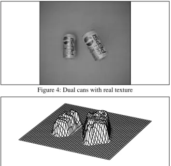
We duplicated the first set of experiments without the checker-board surfaces wrapped around the cans. Instead, we used the actual surfaces of the soda cans under normal lighting conditions. This reduced the number of suitable feature points as well as pro-ducing a non-uniform distribution of feature points across the surface of the cans. Additionally, the surfaces of the cans exhib-ited specularities and reflections that added noise to the displacement measures. The targets (Figure 4) and the result (Fig-ure 5) demonstrate that the additional noise and the distribution of suitable feature points affected the recovery of the curvature on the two surfaces. The errors in these depth measures were typi-cally on the order of a single pixel in nature.

Visual tracking

We conducted multiple runs for the tracking of objects that exhib-ited unknown two- and three-dimensional motion with a coarse estimate of the depth of the objects. The targets for these runs included books, batons, and a computer-generated target dis-played on a large video monitor. During the experiments, we tested the system using targets with linear and curved trajectories. The first experiments were conducted using a book and a baton as targets in order to test the performance of the system both with and without the dynamic pyramiding. These initial experiments served to confirm the feasibility of performing real-time pyramid level switching and to collect data on the performance of the sys-tem under the pyramiding and search optimizing schemes. Figure 6 shows both the target trajectory and manipulator path and the

distance versus time plot from one of these experiments. With the pyramiding and search optimizations, the system was able to track the corner of a book that was moving along a linear trajec-tory at 80 cm/sec. In contrast, the maximum speed reported by Papanikolopoulos [16] was 7 cm/sec, representing an order of magnitude improvement. The dashed line is the target trajectory and the solid line represents the manipulator trajectory. The start of the experiment is in the upper left corner and the end is where the target and manipulator trajectories come together in the lower right. The oscillation at the beginning is due to the switch to higher pyramiding levels as the system compensates for the speed of the target. The oscillations at the end are produced when the target slows to a stop and the pyramiding drops down to the low-est level. This results in the manipulator centering above the feature accurately due to the higher resolution available at the lowest pyramid level.

Once system performance met our minimal requirements, testing proceeded to a computer-generated target where the trajectory and speed could be accurately controlled. The target (a white box) traced either a square or a circle on the video monitor while the PUMA tracked the target

The first experiments traced a square and demonstrated robust tracking in spite of the target exhibiting infinite accelerations (at initial start-up) and discontinuities in the velocity curves (at the corners of the square). The results in Figure 7 clearly show the oscillatory nature of the manipulator trajectory at the points where the velocity curve of the target is discontinuous. The speed of the target in these experiments approached 15 cm/sec.

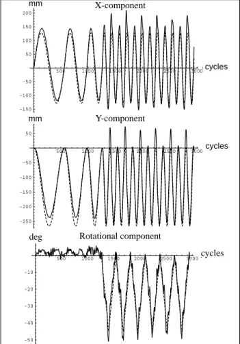
Another set of experiments was conducted using the same setup, only with a target that traced a circle and exhibited Z-axis rota-tions. In these experiments, an appropriate controller was used to track both the translational and the rotational motion. A descrip-tion of this controller can be found in [16].

The resulting data has been separated into the three components of motion. Figure 8 shows the components of translational motion along the X-axis and Y-axis, and the rotational component of motion about the Z-axis.

The target increases speed over the first 3 circular revolutions to lessen the effect of the infinite accelerations mentioned earlier. Also, there is no rotational component of motion during this “wind-up.” The horizontal scale in these plots has a unit of “cycles,” corresponding to the 28 msec cycle of the PUMA’s Uni-mate Computer/Controller.

6. Conclusion

This paper presents robust techniques for the operation of robotic agents in uncalibrated environments. The techniques presented provide ways of recovering unknown workspace parameters using the Controlled Active Vision framework [16]. In particular, this paper presents novel techniques for computing depth maps and Figure 4: Dual cans with real texture

Figure 5: Reconstructed surfaces

1 2 3 4 5 200 400 600 800 100 200 300 400 -600 -500 -400 -300 -200 -100

Figure 6: Spatial plot and distance vs. time plot

mm mm mm sec -150 -100 -50 50 100 150 -150 -100 -50 50 100 150 -150 -100 -50 50 100 150 -150 -100 -50 50 100 150

Figure 7: Target and manipulator paths

mm

mm

mm

for visual tracking through robotic exploration with a camera. For the computation of depth maps, we propose a scheme that is based on the automatic selection of features and design of specific trajectories on the image plane for each individual feature. Unlike similar approaches [8][11][12][18][22], this approach helps to design trajectories that provide maximum identifiability of the depth parameter. During the execution of the specific trajectory, the depth parameter is computed with the help of a simple estima-tion scheme that takes into consideraestima-tion the previous movements of the camera and the computational delays. The approach has been tested and several experimental results have been presented. For visual tracking, we propose a technique based upon earlier work in visual servoing [16] that achieves superior speed and accuracy through the introduction of several performance enhanc-ing techniques. In particular, the dynamic pyramidenhanc-ing technique provides a satisfactory compromise to the speed/accuracy trade-off inherent in static pyramiding techniques. These optimizations apply to various region-based vision processing applications and in our application, provide the speedup required to increase directly the effectiveness of the real-time vision system.

Issues for future research include the automatic selection of the feature window size (an issue discussed in [14]) in order to select a window that has some texture variations, and the implicit incor-poration of the robot dynamics.

7. Acknowledgments

This work has been supported by the Department of Energy (San-dia National Laboratories) through Contract #AC-3752D, the National Science Foundation through Contracts #IRI-9410003 and #CDA-9222922, the Center for Transportation Studies

through Contract #USDOT/DTRS 93-G-0017-1, the Army High Performance Computing Research Center, the 3M Corporation, the Graduate School of the University of Minnesota, and the Department of Computer Science of the University of Minnesota.

8. References

[1] P. Anandan, “Measuring visual motion from image sequences,” Technical Report COINS-TR-87-21, COINS Department, University of Massachusetts, 1987.

[2] S. Brandt, C. Smith, and N. Papanikolopoulos, “The Minnesota Robotic Visual Tracker: a flexible testbed for vision-guided robotic research,” To appear, Proceedings of the IEEE International Conference

on Systems, Man, and Cybernetics, 1994.

[3] J.J. Craig, Introduction to robotics: mechanics and control, Addi-son-Wesley, Reading, MA, 1985.

[4] J.T. Feddema and C.S.G. Lee, “Adaptive image feature prediction and control for visual tracking with a hand-eye coordinated camera,” IEEE

Transactions on Systems, Man, and Cybernetics, 20(5):1172-1183, 1990.

[5] D.B. Gennery, “Tracking known three-dimensional objects,”

Pro-ceedings of the AAAI 2nd National Conference on AI, 13-17, 1982.

[6] J. Heel, “Dynamic motion vision,” Robotic and Autonomous

Sys-tems, 6(3):297-314, 1990.

[7] C.P. Jerian and R. Jain, “Structure from motion—a critical analysis of methods,” IEEE Transactions on Systems, Man, and Cybernetics, 21(3):572-588, 1991.

[8] K.N. Kutulakos and C.R. Dyer, “Recovering shape by purposive viewpoint adjustment,” Proceedings of the IEEE Conference on Computer

Vision and Pattern Recognition, 16-22, 1992.

[9] R.C. Luo, R.E. Mullen Jr., and D.E. Wessel, “An adaptive robotic tracking system using optical flow,” Proceedings of the IEEE

Interna-tional Conference on Robotics and Automation, 568-573, 1988.

[10] D. Marr, Vision, W.H. Freeman and Company, San Francisco, CA, 1982.

[11] L. Matthies, T. Kanade, and R. Szeliski, “Kalman filter-based algo-rithms for estimating depth from image sequences,” International Journal

of Computer Vision, 3(3):209-238, 1989.

[12] L. Matthies, “Passive stereo range imaging for semi-autonomous land navigation,” Journal of Robotic Systems, 9(6):787-816, 1992. [13] P.S. Maybeck, Stochastic models, estimation, and control, Vol. 1, Academic Press, Orlando, FL, 1979.

[14] M. Okutomi and T. Kanade, “A locally adaptive window for signal matching,” International Journal of Computer Vision, 7(2):143-162, 1992. [15] N. Papanikolopoulos, P.K. Khosla, and T. Kanade, “Visual tracking of a moving target by a camera mounted on a robot: a combination of con-trol and vision,” IEEE Transactions on Robotics and Automation, 9(1):14-35, 1993.

[16] N. Papanikolopoulos, “Controlled active vision,” Ph.D. Thesis, Department of Electrical and Computer Engineering, Carnegie Mellon University, 1992.

[17] J.W. Roach and J.K. Aggarwal, “Computer tracking of objects mov-ing in space,” IEEE Transactions on Pattern Analysis and Machine

Intelli-gence, 2(6):583-588, 1979.

[18] C. Shekhar and R. Chellappa, “Passive ranging using a moving cam-era,” Journal of Robotic Systems, 9(6):729-752, 1992.

[19] C. Smith and N. Papanikolopoulos, “Computation of shape through controlled active exploration,” Proceedings of the IEEE International

Conference on Robotics and Automation, 2516-21, 1994.

[20] C. Smith, S. Brandt, and N. Papanikolopoulos, “Controlled active exploration of uncalibrated environments,” Proceedings of the IEEE

Inter-national Conference on Computer Vision and Pattern Recognition,

792-795, 1994.

[21] D.B. Stewart, D.E.Schmitz, and P.K. Khosla, “CHIMERA II: A real-time multiprocessing environment for sensor-based robot control,”

Pro-ceedings of the Fourth International Symposium on Intelligent Control,

265-271, September, 1989.

[22] C. Tomasi and T. Kanade, “Shape and motion from image streams under orthography: a factorization method,” International Journal of

Computer Vision, 9(2):137-154, 1992.

[23] D. Weinshall, “Direct computation of qualitative 3-D shape and motion invariants,” IEEE Transactions on Pattern Analysis and Machine

Intelligence, 13(12):1236-1240, 1991. 500 1000 1500 2000 2500 3000cycles X-Translation Component -150 -100 -50 50 100 150 200 mm

Figure 8: Components of motion

mm cycles 500 1000 1500 2000 2500 3000cycles Y-Translation Component -250 -200 -150 -100 -50 50 mm cycles mm X-component Y-component 500 1000 1500 2000 2500 3000cycles Z-Rotation Component -50 -40 -30 -20 -10 deg cycles deg Rotational component