Monetary Policy Impacts on Cash Crop Coffee and Cocoa Using Structural Vector Error Correction Model

(1)

Monetary Policy Impacts on Cash Crop Coffee and Cocoa Using

Structural Vector Error Correction Model

By

Ibrahim Bamba

Michael Reed

Prepared for presentation at the Meeting of American Agricultural Economists Association, Aug. 1-4 2004 in Denver, Colorado

Ibrahim Bamba is a graduate Student and Michael Reed is a professor. All are in the Department of Agricultural Economics at the University of Kentucky

Copyright 2004 by Ibrahim Bamba and, Michael R. Reed. All rights reserved. Readers may make verbatim copies of this document for non-commercial purposes by any means, provided that this copyright notice appears on all such copies.

(2)

Monetary Policy Impacts on Cash Crops Coffee and Cocoa Using Vector Error Correction Model

Abstract

The international market for the tropical crops coffee and cocoa is marked by high price instability. This paper investigates whether monetary policy disturbances contribute to cocoa and coffee price instability. The econometric evidences point toward high flexibility of the prices of cocoa, arabica coffee, and robusta coffee relative to the industrial price and to the exchange rate. Money supply shock has persistent impact the tropical crop prices and explains an economically significant proportion of their prices variability.

Key words: agricultural prices, volatility, overshooting, cointegration

Introduction

Coffee and cocoa are two agricultural commodities produced mainly in developing countries, exported, and consumed almost entirely in high-income industrialized countries. In several developing countries, cocoa and coffee are the main determinants of aggregate exports and overall economic performance. Statistics from UNCTAD1 help tell the story well. Landlocked African countries such as Burundi and Rwanda rely on coffee for more than 80 percent of their total exports earnings. In Ethiopia, coffee’s share of total export is as high as 79 percent. The economy of Cote d’Ivoire is heavily specialized on cocoa and coffee. Cocoa alone represents 15 percent of Cote d’Ivoire’s GDP and more than 35 percent of her total exports. In Central and South

(3)

America, coffee and cocoa represent the majority of exports for countries such as Columbia, Costa Rica and Haiti.

The international market for cocoa and coffee is marked by high price instability. From January 1990 to December 2003, the coefficient of variation for cocoa price, robusta coffee and arabica coffee were, respectively, 22.5%, 51.1% and 42.8%. The high price volatility of these commodities is explained generally by real economic factors such as production dependence on variable biophysical elements, input subsidies favoring excess supply, irreversible investment due to their perennial nature, low-income elasticity, and inelastic demand. The price volatility of those primary commodities can be attributed to monetary and financial impacts. Changes in monetary policy can affect nominal commodity prices and possibly real commodity prices. This has been the subject of recent literature.

A focus of the literature on monetary impacts has been on overshooting of commodity prices. Frankel (1986) adapted the overshooting hypothesis first introduced by Dornbusch (1976) to agriculture and analytically derived the dynamics of commodity price in a closed economy. By substituting agricultural prices for the exchange rate in Dornbusch’s overshooting model, Frankel (1986 p.345) reported that with an unanticipated and permanent one percent drop in the supply of money “in the long run we would expect all prices to fall by one percent in the absence of new disturbance. But, in the short run industrial good prices are fixed (…) to equilibrate money demand, interest rate rise. But we have an arbitrage condition that must hold in commodity markets: since commodities are storable, the rate of return on Treasury bill can be no greater than the expected rate of increase of the commodity prices minus storage costs2. This means that the spot price of commodities must fall today and must fall by more than the one percent

2_{In his article, Frankel (1986) wrote that the expected increase of commodity prices “plus” storage costs}

could not be greater than the interest rate. Gordon (1987) corrected that flaws and questioned the arbitrage condition in commodity markets.

(4)

that it is expected to fall in the long run.” Frankel (1986) modeled analytically the dynamic path of commodity prices relative of their real or fundamental long-run equilibrium, subsequent to a change in the money market.

Objective of the Study

The objective of this section is to investigate whether monetary factors contribute to coffee and cocoa price instability using structural vector error correction models. A modified empirical framework developed by Saghaian, Reed, and Marchant (2002) is used to test the implication of the overshooting hypothesis for cocoa and coffee subsequent to a monetary shock in the commodity importing country, such as the United States. If cocoa and coffee prices overshoot following a change in the monetary policy of the United States, some evidence of the transmission of monetary policy disturbances from developed countries toward developing countries would have been unraveled. This assertion assumes that developed countries primarily import commodities and developing countries primarily export commodities countries. Specifically the link between changes in the US monetary policy shocks and the volatility of tropical commodity prices is investigated.

Saghaian, Reed, and Marchant (2002) used a four-variable time series model in their empirical investigation of the overshooting model. The four variables were agricultural prices, industrial prices, money supply, and exchange rate. This analysis adds adds a fifth variable to their model, the interest rate, which is naturally part of the system. Unlike Saghaian, Reed, and Marchant (2002), the overshooting of the tropical crops prices is investigated with and without the assumption of money neutrality. With the money neutral assumption, the money supply, the agricultural price, and the industrial price are assumed to move proportionately in the long run. The prices of cocoa and coffee being determined in futures and options exchange market; their relative flexibility and the relative stickiness of industrial good price is examined. The price of industrial good is

(5)

presumed sticky given the prevalence of longer-term contractual arrangements in the industrial sector.

Data and Method

3.1. Method

The application of the overshooting model consists of three steps. In the first step, The stationarity property of each variable is examined using the univariate augmented Dickey Fuller (1979) unit root test and the Philips-Perron (1988) unit root tests. Due to the low reliability of the test for a unit root, additional stationarity tests such as the behavior of the univariate autocorrelation function and time plot are reported. In the second step, the existence of cointegrating relationships among the variables is tested using the Johansen-Juselius procedure. In the third and last step, the vector error correction models are estimated under alternative assumption on the long-run impact of money supply. The validity of the overshooting hypothesis of Dornbusch is assessed by comparing the sign and magnitude of the adjustment parameters for industrial good and the agricultural commodity of interest. The macroeconomic variables, the sticky industrial price, and the agricultural price are all treated as endogenous.

Data

Monthly time series data were collected from 1981:01 to 2003:12. All U.S macroeconomic data are publicly available at the Internet site of the Federal Reserve Bank of St Louis. The conceptual variables, interest rate, exchange rate, money supply, and industrial price, are represented by, respectively, the 3-month Treasury bill rate, the trade-weighted exchange value of U.S. dollar versus currencies of major trading partners3, the M1 money stock, and the producer price index for finished goods (finished goods excluding foods). The level data are shown in Figure 1 through Figure 7. The prices for coffee and cocoa were retrieved, respectively, from the International Coffee

3_{The exchange rate is refereed to exactly as “weighted average of the foreign exchange value of the U.S.}

(6)

Organization and the International Cocoa Organization. Given that coffee is a heterogeneous primary commodity, the price for the most recognized commercial varieties, which are arabica and robusta, are used. The coffee prices are specifically the price of “other mild arabica” and the price of robusta coffee4.

The choice of using the U.S. macroeconomic data is dictated by several considerations. The world prices of cocoa and coffee are denominated in U.S. dollars. The U.S. is the leading importer of both green coffee beans and cocoa beans with, respectively, almost 25 percent and 20 percent of world total imports in 1998 (Food and Agriculture Organization, FAO). The U.S. ranks high in world consumption for coffee and cocoa. In 1998, per capita consumption of coffee and cocoa was, respectively, 4.1 and 2.42 kilograms. Proctor & Gamble, Philip Morris, Mars, and Hershey, all U.S. companies, are major players in the oligopolistic market of goods derived from coffee and cocoa beans. Finally, the New York Board of Trade (NYBOT)5, with London based LIFFE6, is one of two terminal markets for cocoa and coffee. The coffee traded in NYBOT is the arabica variety and the robusta coffee is mainly traded in LIFFE. Coffee is quoted in U.S. dollars on both markets.

Unit root tests

The augmented Dickey-Fuller tests and the Philips-Perron tests are used to detect the presence of a unit root in a time series. The augmented Dickey-Fuller (ADF) assumes that the errors are statistically independent and have a constant variance. To remove the possibility of serial correlation in the residuals when performing the augmented Dickey Fuller test, the literature recommends regressing the dependent variable on a sufficiently

4_{The international coffee organization classifies coffee depending on the country of origin as:}

Colombian mild arabicas, other mild arabicas, Brazilian natural arabicas and robustas

5_{The New York Coffee, Sugar and Cocoa Exchange (CSCE) was the traditional exchanges market for} cocoa and coffee in the United States: since 1998 CSCE is a subsidiary of NYBOT

(7)

large number of lags in order to remove the serial correlation existing in the residuals. Six lags are included in each of our univariate tests for stationarity. The ADF tests involve least square regression of the first difference of the series against the series lagged one period and five other lag difference terms. Moreover, adding five lagged first difference terms in the unit root regression minimized the Schwarz information criterion. The ADF test specified with an intercept is represented as:

t n j j t i i t i t i Z B Z e Z = + + − + ∆

∑

= − − 1 , 1 , 1 0 , α α α (1 ) (2.23)

where ∆is the difference operatorand etis white noise.

The Philips-Perron test is performed to provide additional robustness to the unit root test. Philips-Perron (1988) developed a generalization of the Dickey-Fuller with less restrictive assumptions regarding the distribution of the error terms. The possibility of heteroskedastic errors is accommodated in the Philips-Perron test.

t n j j t i i t i t i Z B Z e Z = + + − + ∆

∑

= − − 1 , 1 , 1 0 , α α α (1 ) (2.24)

The augmented Dickey-Fuller unit root test results and the Philips-Perron results (table 1) reinforce each other. All series are integrated of order one. The unit root tests suggest the natural logarithms of the original series are not stationary but their first differenced are stationary. Because of the low power of the unit root tests, additional investigations of the autocorrelation function and time plot of each series were performed. For a series to be stationary, the autocorrelation function should converge quickly to zero. The autocorrelation function and the visual inspection of the graphical representation of each series support the conclusion reached using the augmented Dickey-Fuller and the Philips-Perron unit root tests. It is concluded that all series are I (1) process and they satisfy the necessary condition for a cointegrated relationship.

(8)

To test for the existence of cointegration between each agricultural price (arabica, robusta, and cocoa) and the U.S. economic variables (industrial price, money supply, exchange rate, and interest rate), the Johansen-Juselius maximum likelihood procedure is used to test the existence of cointegration. The Johansen-Juselius test is a multivariate procedure that can be represented with the following error correction representation:

t p j p t t i t Z Z Z =α +Π + Γ∆ +ε ∆

∑

− = − − 1 1 1 , 0 (2.25)

where Zt is a vector containing the five endogenous variables, which include the

agricultural price (either cocoa or coffee), the money supply, the exchange rate, the interest rate and the industrial price. The matrix Γi contains the short-run coefficients

among the variables in the system, εt is white noise and the matrix Π contains the

information on the eventual cointegration relations among the series in the vector Zt. Equation 2.25 can be rewritten as:

t p j t p t i t Z Z Z =α −αβ + Γ∆ +ε ∆

∑

− = − − 1 1 1 , 0 (2.26)

The reduced rank matrix Π captures the long-run stationary relationship among the variables. When the matrix Π has a reduced ranked there is a factorization Π = αβ’, where the matrix β contains the r cointegrating relations and the matrix α contains the adjustments parameters in the vector error correction model (VECM), or the short-run overshooting parameters in the model. Both β and α are 5 x 2 matrices in this application. The stationary error correction terms are ΠZt-1 =αβZt-1. The error correction

part and the VAR part can accommodate different trend specifications.

Regarding the cointegrating equation (αβ Zi,t−1) and the deterministic components (α0) to include in the error correction representation, Johansen (1995) considered five

possible trend specifications. Johansen (1994) demonstrated that the inclusion of intercepts in the vector Zt of a differenced series implies that the nonstationary level

(9)

variables have a linear trend. When the vector Zt of differenced series and the

cointegrating equations have linear trends, the nonstationary variables have quadratic trend behavior. Below are the five possible specifications:

1. The vectors of level data, Zt, have no deterministic trends and the

cointegrating equations do not have intercepts:

t p j p t t i t Z Z Z =Π + Γ∆ +ε ∆

∑

− = − − 1 1 1 , , where Π =αβ (2.27)

2. The vectors of level data Zt have no deterministic trends and the cointegrating

equations have intercepts:

t p j p t t i t Z Z Z =Π + Γ∆ +ε ∆

∑

− = − − 1 1 1 , , where Π = α(β Zt-1+ ρ0) (2.28)

3. The vectors level data Zt have a linearly trend and the cointegrating equations

have only intercepts:

t p j t p t i t Z Z Z =α +Π + Γ∆ +ε ∆

∑

− = − − 1 1 1 , 0 , where Π = α(β Zt-1+ ρ0) (2.29)

4. The vectors of level data Zt have and the cointegrating equations have linear

trends: t p j t p t i t Z Z Z =α +Π + Γ∆ +ε ∆

∑

− = − − 1 1 1 , 0 , where Π= α(β Zt-1+ ρ0+ ρ1t) (2.30) 5. The vector Zt of level data have quadratic trends and the cointegrating

equations have linear trends:

t p j p t t i t t Z Z Z =α +α +Π + Γ∆ +ε ∆

∑

− = − − 1 1 1 , 1 0 , where Π= α(βZt-1+ ρ0+ ρ1t) (2.31) The Johansen-Juselius maximum likelihood procedure tests the rank of Π by testing the number of non-zero eigenvalues or characteristic roots. Conceptually, four possible scenarios can arise.

(10)

1- The rank of Π= zero, the variables in the vector Ztisintegrated of order one; they

are I (1) but no cointegrated.

2- The rank of Π = five, this is the case of full rank matrix which, implies all variables are I (0).

3- The rank of Π = one, there is only one linear independent row in Π or one cointegrating vector.

4- The rank of Π = r, 1 < r < 5, there are r linearly independent rows in Π or r

cointegrating vectors.

Two null hypotheses are employed to test for the existence and the number of cointegrated relationships in the Johansen methodology. They are referred to in the literature as λ-trace or the trace statistic test and λ-max test or the maximal eigenvalue test7. Both the trace test and the maximal eigenvalue test are applied using a sequential process. The null hypothesis for the trace statistic is the existence of r cointegrating relations versus the absence of r cointegrated relationships. The procedure begins by testing whether there is no cointegration (r = 0). The rejection of the null hypothesis leads to testing higher orders of cointegration. The second test statistic (λ-max test) is used to test the null hypothesis that there are at most r cointegrating relationships versus the alternative of r + 1 cointegrating relationship.

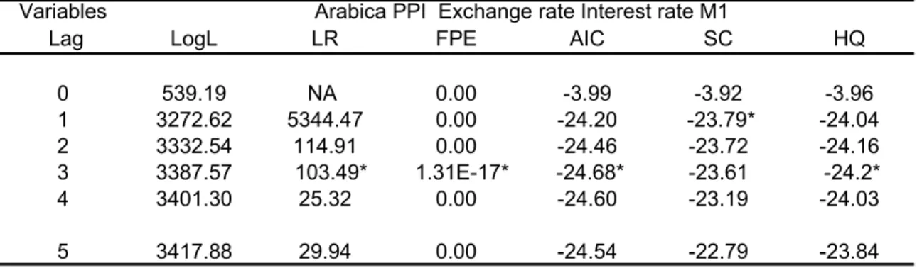
Prior to performing the Johansen-Juselius maximum likelihood test for cointegration, the optimal lag order to include must be determined. The determination of the lag length is carried out done by using numerous diagnostic statistics such as the final prediction error (FPE), Schwarz information criterion (SC), the sequential modified likelihood ratio (LR) test, the Akaike information criterion (AIC), and the Hannan-Quinn information criterion (HQ). The diagnostic statistics are presented in table 2, 3, and 4. They indicate that the lag order three results in optimal values for four out five

7_{The asymptotic distributions of the trace and maximal eigenvalue test depend on the specification used for}

(11)

multivariate diagnostic statistics for the system containing the given tropical crop price (cocoa, arabica or robusta) and the U.S. macroeconomic variables (i.e., money supply, interest rate, exchange rate, industrial price).

The cointegration tests are performed using each of the five possible deterministic trend specifications of Johansen (1995). The summary for all specifications of cointegration tests is presented in table 5. Although the numbers of cointegrating vectors determined with the trace test and the maximal eigenvalue test appear sensitive to the specification of the data generating process, a least one cointegrating relationship is found at the 5% confidence level, regardless of the multivariate specification used for the Johansen rank test. The specification represented by the equation 2.31 excepted, the specifications represented by equations 2.27, 2.28, 2.29 and 2.30 suggest the presence of two cointegrating vectors.

The presence of more than one cointegrating relationship linking the U.S. macroeconomic variables (i.e. money supply, interest rate, exchange rate, industrial price) and each of the commodity price of interest (i.e. robusta coffee, arabica coffee, or cocoa), using the specification suggest the presence of 2 linear combinations of non-stationary series yielding a non-stationary relationship between the variables. The existence of multiple cointegrating vectors implies that “it may not be possible to identify the behavioral relationships from the reduced-form relationships” (Enders, 2003 p.323). For example, with two cointegrating vectors, there is an independent cointegrating vector for each combination of four variables. To provide meaningful economic interpretation of the results, the system needs to be identified. According to Johansen and Juselius (1994), for a number r of cointegrating vectors, r² restrictions are needed to identify the cointegrating vector β without changing the likelihood function. To identify a system containing two cointegrating vectors, there must be at least two restrictions imposed on each cointegrating vector.

(12)

Empirical Results

4.1. VECM Results using the Unrestricted SRM method

Similar to the cointegration test, the estimation of the error correction model requires one to specify the deterministic components in the multivariate differenced time series and in the cointegrating relationships. In the absence of prior theoretical guidance, this is done by choosing the specification that maximizes the log-likelihood function. The specification (2.31), where the variables in the multivariate nonstationary time series, have quadratic trends is found to maximize the log-likelihood function. Hence, the estimation of the error correction models is carried out using the specification that include in linear trend in both the cointegrating relationships and the first differenced vector autoregressive component. Furthermore, given that all other deterministic trend specifications outlined by Johansen (1944) are nested in the specification with quadratic trends, misspecification bias should be minimized by using that specification. The cointegration tests with the quadratic trend specification are presented in the table 6. With the quadratic trend specification, only one cointegrating vector is found at the higher 5% confidence level. There is thus no need for arbitrary identification and the only requirement is to normalize the estimates with one of the variables. In this investigation, all estimates are normalized with respect to the agricultural commodity price. The unique cointegrating vector is interpreted as the long-run equilibrium relationship (Engle and Granger, 1987). The estimates of the unrestricted adjustment coefficient for the agricultural commodity and the industrial good the normalized cointegrating vector are then used to assess the inference of the overshooting hypothesis.

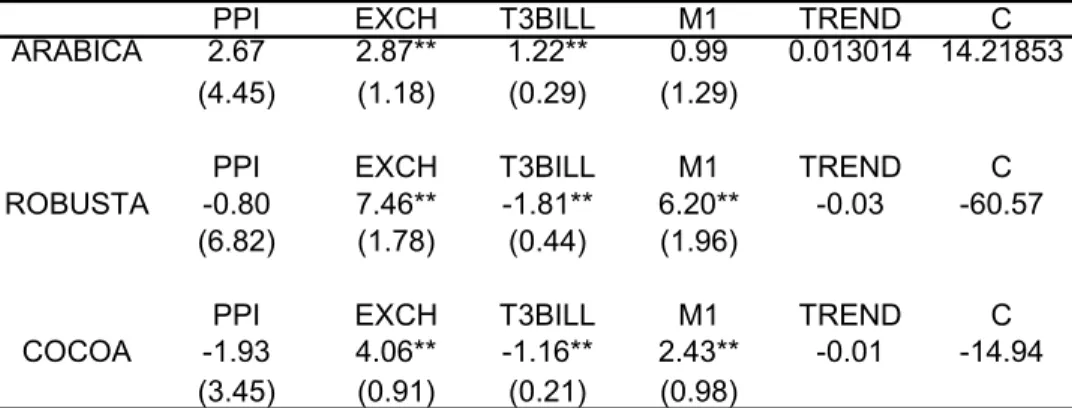
Table 7 present the results obtained with the identification method of SRM. In the model containing robusta coffee price, the long-run parameters estimates for the impact of U.S money supply on robusta price, arabica price and cocoa price are, respectively,

(13)

6.20%, 0.99%, and 2.43%8. The hypothesis that money is neutral is rejected for robusta coffee at the 5% significance level. The hypothesis of money neutrality is not rejected for models that include cocoa and arabica coffee as the agricultural price. A 1% increase in money supply leads to a long-run increase of cocoa price, robusta coffee, and arabica coffee price by, respectively, 6.20%, 0.99%, and 2.43%.

The long-run relationship between money supply and the nominal price on the agricultural commodities seems to be sensitive to the good considered. The sign of the coefficients measuring the long-run impact of money supply on cocoa, robusta or arabica coffee are consistent with our expectations. An expansionary monetary policy positively affects the prices of robusta coffee, arabica coffee, and cocoa. Yet the effect of money supply on robusta coffee price is unusually large.

The adjustment parameter for the agricultural commodity price in the cointegrating vector is viewed as the overshooting parameter for the commodity price because it represents the deviation from the long-run equilibrium relationship. Likewise, the adjustment parameter for the industrial product price is its overshooting parameter. The agricultural price overshoots in the short-run when the absolute value of its adjustment parameter is greater than the adjustment parameter for the industrial good. The adjustment parameters are presented in table 8.

In the cocoa model, the overshooting coefficient is -1.79% and the overshooting coefficient for the industrial good price is 0.08%. For robusta coffee the overshooting coefficient is -1.86% and the coefficient for industrial good price is 0.04%. Finally, for arabica coffee, the overshooting coefficient is 3.22% and the coefficient of the industrial good is close to zero. These empirical findings conform to the overshooting findings of Frankel and SRM for agricultural goods. The overshooting parameters for all three agricultural goods are statistically different from zero and greater than the overshooting

8_{Johansen (2002) demonstrated that the long-run coefficients in a cointegrating relationship could be called}

(14)

parameters for industrial good price. All of the coefficients for industrial good price are insignificant. Arabica coffee, robusta coffee price, and cocoa prices are therefore flexible and react faster to macroeconomic disturbances, while the industrial good are sticky.

To summarize the results, the signs of the overshooting parameters for the imported commodities are negative as expected; they indicate that price must fall after a macroeconomic shock to reestablish the long run equilibrium among the variables. Even though the results for cocoa and arabica coffee appear reasonable, the plausibility of the long run impact of macroeconomic variables such as money supply and exchange rate on robusta price is questionable. For example, the high impact of money supply on robusta price does not appear to match the observed downward trend. To improve on the SRM model, the assumption of money neutrality is imposed and the behaviors of the agricultural commodity price and industrial good price are revisited.

4.2. Results with Long-Run Neutral Money Restrictions

In the SRM model estimated earlier, money supply is allowed to have real effects on goods price in both the short-run and in the long run. An alternative empirical verification of the short-run effect of money on industrial and agricultural prices in the overshooting framework requires one to posit explicitly that money is neutral in the long-run (Robertson and Orden, 1990). Hence, the long-long-run impact of money supply on industrial good price and agricultural prices (robusta coffee, arabica coffee, and cocoa) are restricted to unity for this part of the analysis. The appropriateness of the restriction will also be tested.

The tests for the long-run neutrality of money supply on the tropical beverage prices are conducted using the likelihood ratio statistic. The results presented in table 9 show that the hypothesis of money neutrality cannot be rejected at the 5% level of significance for all three systems. The likelihood ratio test is performed using the asymptotic chi-square distribution. The sizes of the impacts of other macroeconomic

(15)

variables, such as the exchange rate, on agricultural good are sensible, specifically in the robusta coffee model. For instance, in the unrestricted SRM model, an increase of the exchange rate by one percent increases the price of robusta price by more than 7.45%. With the long-run money neutrality assumption, the same augmentation of the exchange rate leads to a 3.30% increase in the price of robusta coffee. In all the three models, the long-run impacts of exchange rate and interest rate on the tropical commodity prices are statistically significant. The long-run intercept and the time trend coefficient are negative. These suggest the possible existence of negative trend between the tropical crop prices and the United States economic variables included here.

The adjustment parameters obtained when long-run money neutrality is imposed are presented in table 10. The results still indicate that the prices of cocoa and both types of coffee overshoot. Their overshooting parameters are significantly different from zero and their magnitudes are greater than the overshooting parameter for the sticky industrial price. The adjustment coefficients for the industrial good price remain insignificant in all three models. Therefore, cocoa price and coffee prices return to their long-run equilibrium faster than the industrial good price. Arabica coffee price reacts more strongly to the United States market information than robusta coffee or cocoa price. The monthly overshooting parameter for arabica coffee and cocoa are respectively -3.41% and -2.57%. This might be due to the fact that arabica price is taken from the NYBOT whereas robusta is taken from the LIFFE in London, England.

The overshooting coefficients obtained when the assumption of neutral money is imposed are similar to the ones obtained with the SRM method. The degree of overshooting of both types of coffee is slightly higher when money is assumed neutral and the arabica price appears to overshoot more than the robusta price to change in the US macroeconomic variables. For cocoa, the degree of overshooting is marginally lower with money neutrality than with the SRM model. As expected, the signs of the

(16)

adjustment coefficients on money supply and interest are different. The interest rate, being the opportunity cost of money, should move prices in the opposite direction of money supply changes. In the unrestricted SRM model, this did not hold for all cases, but the interest rate coefficient was always the opposite sign from the money supply coefficient in the second experiment. Therefore, the restricted SRM representations improve on the estimation of the dynamic relationship between the United States macroeconomic variables and the price of tropical beverage coffee and cocoa by yielding plausible elasticity estimates.

4.3. Impulse Response and Variance decomposition

Next, the impact of money supply on the volatility of cocoa and coffee price is investigated using innovations accounting techniques such as the impulse response functions and the variance decomposition. The impulse response function measure the effect of a shock to one variable another variable for a number of periods ahead with other variables held constant.

Examination of the impulse response helps trace the effects of monetary shocks on current and futures value of coffee and cocoa prices with and without the assumption money neutrality. The responses functions are obtained using the generalized impulse response technique of Pesaran and Shin (1998), which is available in the Eviews software. Pesaran and Shin adapted the Cholesky orthogonalization technique to obtain impulse response functions that are independent of the variables ordering, and therefore, giving a unique dynamic behavior. The Cholesky decomposition technique allows one to single out the individual shock effects when the elements in the residuals covariance matrix are contemporaneously correlated.

Because the impulse response function to a standard deviation of money supply innovation on the tropical commodities prices are nearly analogous with and without the money neutrality assumption, only the response function for the restricted model is presented. The dynamic responses of the agricultural and industrial good prices to one

(17)

standard deviation monetary shock are presented from figure 8 to figure 109. The responses functions confirm the statistical results obtained previously. An exogenous one standard deviation monetary supply shock has a long lasting, volatile, negative then positive impact on each the tropical commodity price. The initial impact of money supply on each the agricultural price is a negative jump that stretch over three, four, and five months, respectively for cocoa, robusta coffee, and arabica coffee. The prices then rebound after reaching a minimum level and increase steadily toward a position long-run equilibrium. A longer-term impact of the money supply shock on the tropical commodities prices is relatively small, less than 2.00% in each case, but the monetary shock a persistent effect on commodity price. For example, none of the responses functions reaches a stable level prior to a 50-month forecast horizon.

The responses of the industrial good price to a monetary shock are clearly negligible in the three models. Thus, the agricultural commodity price responds faster to money supply shock than the industrial good price. Overall, imposing the assumption of money neutrality does not notably change the dynamic path of the commodities prices.

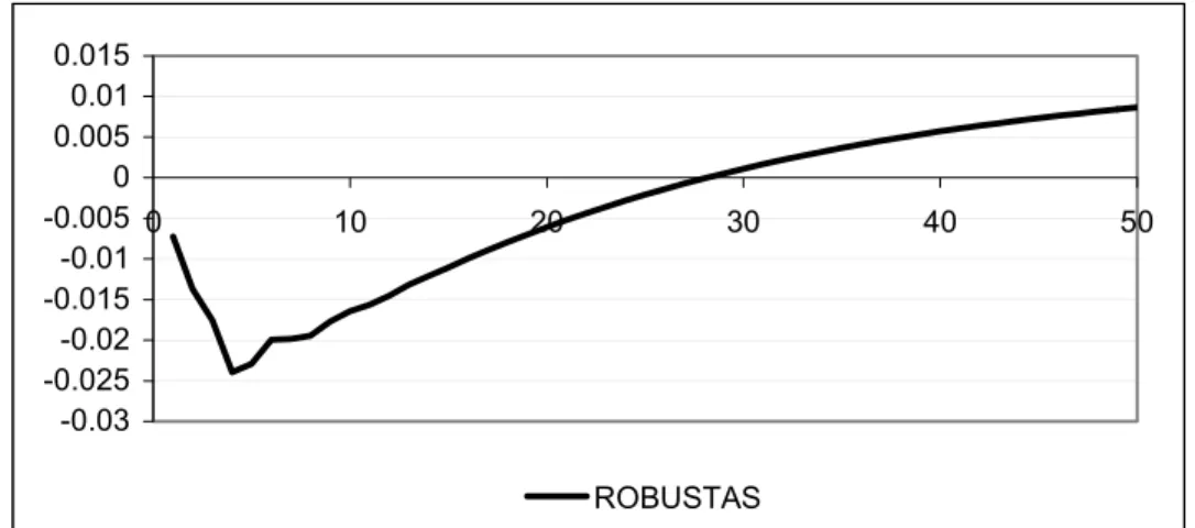
Using the case of robusta coffee, for which the hypothesis of money neutrality was rejected with the SRM model, as illustration, a one standard deviation innovation originating from the money supply results in a negative drop in price which reaches a minimum level at -2.40% after four months (See Figure 11 for an amplified plot). Then a reversal occurs, the response become positive after 29 months and kept increasing until a new long-run positive equilibrium level is reached at 1.36%.

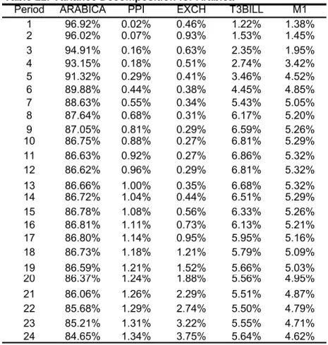
To assess the percentage variation in the tropical good prices that originates from the other variables, their forecast error is decomposed. The multivariate covariance matrix in VAR being in general non-diagonal, the Cholesky lower triangular ordering is used to compute the variance decomposition. The ordering imposed goes from the money supply to the agricultural price. Specifically, the money supply is followed by the interest

(18)

rate, which is followed by the exchange rate, which is followed by the industrial price, which is followed by the agricultural price. The variance decomposition results under money neutrality are presented in tables 11, 12, and 13. In all cases, the variation in each of the variable forecast error is explained by their own shock at 80% or higher with a 12 months forecast horizon. This suggests that the dynamics of cocoa or coffee prices are mainly functions of their respective market fundamentals such as supply and demand conditions. At the 12-month forecast horizon, the United States monetary instruments, such as the money supply and the interest rate, jointly affect coffee prices more than they affect cocoa price. The contribution of the United States monetary instruments in the variance of the tropical crop is higher for arabica than for robusta coffee price and cocoa price. With a 24-month forecast horizon, the joint contribution money supply and interest exceed 10% for each of the agricultural price.

Summary and Conclusion

In this paper, the vector error correction methodology is used to analyze the impacts of United Stated monetary policy on coffee and cocoa prices using a modified conceptual and analytical framework of Saghaian, Reed, and Marchant. The results of this analysis shed light on overshooting of agricultural prices for two important crops for less developed countries, cocoa and coffee. The econometric evidence points toward overshooting of cocoa and coffee prices in the short-run. The price of cocoa and coffee respond faster to money supply shock than the industrial good price. Thus, arabica coffee price, robusta coffee price and cocoa price appear more flexible than industrial good price. The tropical crop prices also respond faster than the exchange rate, which is also traded in transparent auction market. The impulse response functions of arabica coffee price, robusta coffee price and cocoa price to money supply change are marked by their initial negative impact and their persistent positive long-run effect. The impulse responses functions signal that the long-run impacts of money supply sock on the tropical beverage crop prices are permanent. The dynamic paths of the tropical commodity prices

(19)

obtained with and without the money neutrality assumption were very similar. The variance decomposition results indicate that stochastic changes in the fundamental market conditions each tropical crop are the main sources of volatility. However, United Stated monetary policy instruments are found to explain an economically significant proportion of the variation in the forecast error of coffee and cocoa price.

The flexibility and overshooting of the tropical crops prices have important implication for developing countries. In the 1970’s, international commodity agreements and marketing boards have unsuccessfully attempted to stabilize the prices of coffee and cocoa price. Nowadays, market-based instruments such futures and options hedging, are advocated as efficient and effective alternative to mitigate the price instability of these tropical beverage crop. Besides of challenges such transaction costs, exchange rate risk, and the basis risk, arising when one attempt to use markets located in New York and London to hedge her outputs price from a developing country, there is a need to account for the role of changing macroeconomic policy.

(20)

References:

Dornbusch, R. “Expectations and Exchange rates Dynamics.” Journal of Political Economics 84 (1976): 1161-76.

Enders W. “Applied Econometric Time Series” Second edition 2003, John Wiley, and Sons, Inc.

Eviews User’s Guide Version 4 for Windows 9x, NT 4.0, 2000 and XP. Quantitative Micro Software Irwin CA 2000.

Fisher L., P. L. Fackler and D. Orden. “Long-run Identifying Restriction for an Error Correction Model of New Zealand Money, Prices and Output.” Journal of International Money and Finance 14 (1995): 127-147.

Frankel, A. J. “Expectation and Commodity Price Dynamics: The Overshooting model” American Journal of Agricultural Economics 68 :( 1986): 343-348.

Johansen, S. “The Role of the Constant and Linear Terms in Cointegration Analysis of Nonstationary Variables.” Econometrica Reviews 13 (1994): 205-229.

Johansen, S. “Likelihood-based Inference in Cointegrated Vector Autoregressive Models.” Oxford University Press 1995.

Johansen, S. “The Interpretation of Cointegrating Coefficients in the Cointegrated Vector Autoregressive Model.” Working Paper No 14, Department of Theoretical Statistics, University of Copenhagen, Oct. 2002.

Johansen, S. and K. Juselius. “Testing Structural Hypothesis in a Multivariate Cointegration Analysis of the PPP and UIP for the UK.” Journal of Econometrics 53

(1992).

Pesaran, M.H. and Y. Shin. “Generalized impulse response analysis in linear Multivariate models” Economics Letters 58 (1998):17-29.

(21)

Saghaian, S. H., M. Reed and M. A. Marchant. “Monetary Impacts and Overshooting of Agricultural Prices in an Open Economy.” American Journal of Agricultural Economics 84 1 (2002): 90-103.

(22)

Tables and figures Table 1. Unit Root Tests

Level First ∆ Level First ∆

Robusta -3.46 -8.72 -1.40 -12.46 Arabica -1.85 -7.10 -2.10 -12.90 Cocoa -2.04 -7.76 -2.04 -13.14 M1 -3.19 -6.44 -2.78 -18.56 PPI -0.94 -7.12 -1.59 -12.76 Interest rate -0.37 -5.66 0.23 -10.99 Exchange rate -1.27 -7.30 -1.26 -11.49

∆ represents the difference operator

MacKinnon 1% critical values for rejection of hypothesis of a unit root is -3.45

Augmented Dickey-Fuller Philips-Perron

Table 2: VAR Lag length selection criteria

Variables

Lag LogL LR FPE AIC SC HQ

0 539.19 NA 0.00 -3.99 -3.92 -3.96 1 3272.62 5344.47 0.00 -24.20 -23.79* -24.04 2 3332.54 114.91 0.00 -24.46 -23.72 -24.16 3 3387.57 103.49* 1.31E-17* -24.68* -23.61 -24.2* 4 3401.30 25.32 0.00 -24.60 -23.19 -24.03 5 3417.88 29.94 0.00 -24.54 -22.79 -23.84

* indicates lag order selected by the criterion

LR: sequential modified LR test statistic (each test at 5% level) FPE: Final prediction error

AIC: Akaike information criterion SC: Schwarz information criterion

Arabica PPI Exchange rate Interest rate M1

Variables

0 508.65 NA 0.00 -3.76 -3.69 -3.73 1 3310.93 5479.08 0.00 -24.48 -24.08* -24.32 2 3371.82 116.78 0.00 -24.75 -24.02 -24.46 3 3424.56 99.18 9.96E-18* -24.96* -23.89 -24.53* 4 3440.52 29.43 0.00 -24.89 -23.49 -24.33 5 3457.00 29.77 0.00 -24.83 -23.09 -24.13

AIC: Akaike information criterion SC: Schwarz information criterion HQ: Hannan-Quinn information criterion

(23)

Variables

0 625.19 NA 0.00 -4.63 -4.56 -4.60 1 3364.78 5356.50 0.00 -24.89 -24.48* -24.72 2 3425.70 116.85 0.00 -25.15 -24.42 -24.86 3 3480.24 102.56* 6.57E-18* -25.37* -24.30 -24.94* 4 3490.62 19.13 0.00 -25.27 -23.86 -24.70 5 3510.74 36.34 0.00 -25.23 -23.49 -24.53

AIC: Akaike information criterion SC: Schwarz information criterion HQ: Hannan-Quinn information criterion

Cocoa PPI Exchange rate Interest rate M1

Table 5: Summary of all Five sets of Johansen assumptions

Data Trend: None None Linear Linear Quadratic

VAR No Intercept Intercept Intercept Intercept Intercept

EC No Trend No Trend No Trend Trend Trend

Variables Trace 2 2 2 2 1 Max-Eig 2 2 2 2 1 Variables Trace 2 2 2 1 1 Max-Eig 2 2 1 1 1 Variables Trace 2 2 2 2 1 Max-Eig 2 2 2 1 1

Number of Cointegrating Relations at 5% significance level Max-Eig=maximum eigenvalue

VAR=Vector autoregressive and EC=error correction

ROBUSTA PPI EXCH T3BILL M1 ARABICA PPI EXCH T3BILL M1

COCOA PPI EXCH T3BILL M1

Table 6: Cointegration test using the Quadratic determinic trend

Model Robusta + Arabica + Cocoa + 5 % CV 10% CV

None 89.38** 93.70** 95.19** 77.74 73.4

At most 1 42.44 51.32* 49.56 54.64 50.74

At most 2 16.63 21.23 23.45 34.55 31.42

At most 3 5.54 7.01 7.89 18.17 16.06

At most 4 1.84 3.36 3.21 3.74 2.57

Model Robusta + Arabica + Cocoa + 5 % CV 10% CV

None 46.94** 42.38** 45.63** 36.41 33.74

At most 1 25.81 30.08* 26.11 30.33 27.76

At most 2 11.09 14.22 15.57 23.78 21.53

At most 3 3.70 3.65 4.68 16.87 14.84

At most 4 1.84 3.36 3.21 3.74 2.57

(**) and (*) denote significance at 5% and 10% CV is for critical value from Osterwald-Lenum (1992) + denotes the US variables, PPI, EXCH, T3BILL, M1

Trace statistic

(24)

Table 7. Long-Run Parameters with SRM Model

PPI EXCH T3BILL M1 TREND C

ARABICA 2.67 2.87** 1.22** 0.99 0.013014 14.21853

(4.45) (1.18) (0.29) (1.29)

ROBUSTA -0.80 7.46** -1.81** 6.20** -0.03 -60.57

(6.82) (1.78) (0.44) (1.96)

COCOA -1.93 4.06** -1.16** 2.43** -0.01 -14.94

(3.45) (0.91) (0.21) (0.98)

( ), **, and C denote the standard error, the significance at 5% and the intercept

Table 8. Error Correction with SRM Model

∆ARABICA ∆PPI ∆EXCH ∆T3BILL ∆M1

εarabica,t-1 -3.22%** 0.00% 0.55%** 0.51% -0.59%**

(0.009) (0.001) (0.002) (0.006) (0.001)

∆ROBUSTA ∆PPI ∆EXCH ∆T3BILL ∆M1

εrobusta,t-1 -1.86%** 0.04% 0.45%** 0.13% -0.29%**

(0.004) (0.00) (0.001) (0.003) (0.001)

∆Cocoa ∆PPI ∆EXCH ∆T3BILL ∆M1

εcocoa,t-1 -1.79** 0.08% 0.89%** -0.40% -0.71%**

(0.008) (0.001) (0.002) (0.007) (0.003)

( ) and ** denote the standard error and the significance at 5%

Table 9. Long-Run Parameters with Restricted Model

ARABICA 1 2.58** 0.86** 1 -0.01 -15.83

(0.69) (0.26)

LR test for M1 = ARABICA = PPI = 1 chi-square = 0.069

Probability =0.97

ROBUSTA 1 3.31** -1.37** 1 -0.02 -18.09

(0.88) (0.32)

LR test for M1 = ROBUSTA = PPI = 1 chi-square = 4.978

Probability = 0.08

COCOA 1 3.15** -1.05** 1 -0.01 -15.49

(0.49) (0.21)

LR test for M1 = COCOA = PPI = 1 chi-square = 1.29

Probability = 0.52

(25)

Table 10. Error Correction with SRM restricted Model

∆ARABICA ∆PPI ∆EXCH ∆T3BILL ∆M1

εarabica,t-1 -3.41%** -0.01% 0.59%** 0.52% -0.63%** (0.006) (0.001) (0.002) (0.006) (0.001)

∆ROBUSTA ∆PPI ∆EXCH ∆T3BILL ∆M1

εrobusta,t-1 -2.57%** 0.02% 0.52%** 0.81% -0.44%** (0.006) (0.004) (0.001) (0.003) (0.001)

∆Cocoa ∆PPI ∆EXCH ∆T3BILL ∆M1

εcocoa,t-1 -2.43%** 0.09% 0.95%** 0.13% -0.94%** (0.009) (0.006) (0.002) (0.008) (0.002) ( ) and ** denote the standard error and the significance at 5%

Table 11: Variance Decomposition for Arabica

Period ARABICA PPI EXCH T3BILL M1

1 96.92% 0.02% 0.46% 1.22% 1.38% 2 96.02% 0.07% 0.93% 1.53% 1.45% 3 94.91% 0.16% 0.63% 2.35% 1.95% 4 93.15% 0.18% 0.51% 2.74% 3.42% 5 91.32% 0.29% 0.41% 3.46% 4.52% 6 89.88% 0.44% 0.38% 4.45% 4.85% 7 88.63% 0.55% 0.34% 5.43% 5.05% 8 87.64% 0.68% 0.31% 6.17% 5.20% 9 87.05% 0.81% 0.29% 6.59% 5.26% 10 86.75% 0.88% 0.27% 6.81% 5.29% 11 86.63% 0.92% 0.27% 6.86% 5.32% 12 86.62% 0.96% 0.29% 6.81% 5.32% 13 86.66% 1.00% 0.35% 6.68% 5.32% 14 86.72% 1.04% 0.44% 6.51% 5.29% 15 86.78% 1.08% 0.56% 6.33% 5.26% 16 86.81% 1.11% 0.73% 6.13% 5.21% 17 86.80% 1.14% 0.95% 5.95% 5.16% 18 86.73% 1.18% 1.21% 5.79% 5.09% 19 86.59% 1.21% 1.52% 5.66% 5.03% 20 86.37% 1.24% 1.88% 5.56% 4.95% 21 86.06% 1.26% 2.29% 5.51% 4.87% 22 85.68% 1.29% 2.74% 5.50% 4.79% 23 85.21% 1.31% 3.22% 5.55% 4.71% 24 84.65% 1.34% 3.75% 5.64% 4.62%

(26)

Table 12: Variance Decomposition for Robusta

Period ROBUSTA PPI EXCH T3BILL M1

1 98.43% 0.00% 0.27% 0.23% 1.07% 2 97.46% 0.03% 0.13% 0.41% 1.95% 3 96.41% 0.06% 0.30% 0.58% 2.66% 4 94.91% 0.08% 0.30% 0.89% 3.82% 5 94.12% 0.11% 0.24% 1.18% 4.35% 6 93.81% 0.15% 0.20% 1.39% 4.46% 7 93.60% 0.17% 0.19% 1.48% 4.57% 8 93.52% 0.18% 0.20% 1.45% 4.65% 9 93.56% 0.19% 0.25% 1.35% 4.65% 10 93.61% 0.20% 0.33% 1.24% 4.62% 11 93.60% 0.20% 0.46% 1.15% 4.59% 12 93.54% 0.20% 0.62% 1.10% 4.54% 13 93.40% 0.20% 0.83% 1.10% 4.47% 14 93.16% 0.20% 1.09% 1.17% 4.39% 15 92.80% 0.20% 1.38% 1.31% 4.30% 16 92.34% 0.19% 1.72% 1.54% 4.21% 17 91.75% 0.19% 2.10% 1.85% 4.11% 18 91.05% 0.18% 2.52% 2.24% 4.01% 19 90.23% 0.18% 2.97% 2.72% 3.90% 20 89.29% 0.17% 3.46% 3.28% 3.79% 21 88.25% 0.17% 3.97% 3.93% 3.68% 22 87.11% 0.16% 4.51% 4.64% 3.57% 23 85.88% 0.16% 5.07% 5.43% 3.47% 24 84.56% 0.15% 5.65% 6.27% 3.36%

Table 13: Variance Decomposition for Cocoa

Period COCOA PPI EXCH T3BILL M1

1 97.86% 0.00% 0.60% 1.01% 0.53% 2 98.75% 0.02% 0.52% 0.41% 0.30% 3 98.31% 0.22% 0.50% 0.51% 0.46% 4 98.52% 0.21% 0.43% 0.47% 0.37% 5 98.76% 0.18% 0.36% 0.40% 0.31% 6 98.88% 0.15% 0.32% 0.38% 0.27% 7 98.82% 0.14% 0.32% 0.49% 0.23% 8 98.58% 0.12% 0.38% 0.71% 0.22% 9 98.20% 0.11% 0.49% 0.99% 0.21% 10 97.67% 0.10% 0.66% 1.37% 0.20% 11 96.97% 0.09% 0.88% 1.84% 0.21% 12 96.14% 0.09% 1.16% 2.39% 0.22% 13 95.19% 0.08% 1.48% 3.01% 0.24% 14 94.13% 0.08% 1.84% 3.68% 0.27% 15 92.98% 0.08% 2.23% 4.41% 0.30% 16 91.76% 0.07% 2.65% 5.17% 0.34% 17 90.49% 0.07% 3.10% 5.96% 0.38% 18 89.17% 0.07% 3.55% 6.78% 0.42% 19 87.83% 0.07% 4.02% 7.61% 0.47% 20 86.48% 0.07% 4.50% 8.44% 0.52% 21 85.12% 0.07% 4.98% 9.27% 0.56% 22 83.76% 0.07% 5.46% 10.10% 0.61% 23 82.42% 0.07% 5.93% 10.92% 0.66% 24 81.09% 0.07% 6.40% 11.73% 0.71%

(27)

Figure 8: Impulse response to one standard deviation of M1 shock using Money Neutral Model -0.03 -0.02 -0.01 0 0.01 0 20 40 60 80 100 120 ARABICA PPI

Figure 9: Impulse response to one standard deviation of M1 shock using the money neutral -0.03 -0.02 -0.01 0 0.01 0.02 0 20 40 60 80 100 120 ROBUSTAS PPI

Figure 10: Impulse Response to one standard deviation of M1 shock using the Money Neutral model -0.007 -0.002 0.003 0.008 0.013 0.018 0 20 40 60 80 100 120 COCOA PPI

Figure 11: Impulse Response to one standard deviation of M1 shock using the Money Neutral model -0.03 -0.025 -0.02 -0.015 -0.01 -0.005 0 0.005 0.01 0.015 0 10 20 30 40 50 ROBUSTAS