Volume 33
Number 471
Changes in supply functions and supply
elasticities in hog production
Article 1
November 1959
Changes in supply functions and supply elasticities
in hog production
Gerald W. Dean
Iowa State University of Science & Technology
Earl O. Heady
Iowa State University of Science & Technology
Follow this and additional works at:
http://lib.dr.iastate.edu/researchbulletin
Part of the
Agriculture Commons
,
Economics Commons
, and the
Sociology Commons
This Article is brought to you for free and open access by the Iowa Agricultural and Home Economics Experiment Station Publications at Iowa State University Digital Repository. It has been accepted for inclusion in Research Bulletin (Iowa Agriculture and Home Economics Experiment Station) by an authorized editor of Iowa State University Digital Repository. For more information, please [email protected].
Recommended Citation
Dean, Gerald W. and Heady, Earl O. (1959) "Changes in supply functions and supply elasticities in hog production,"Research Bulletin (Iowa Agriculture and Home Economics Experiment Station): Vol. 33 : No. 471 , Article 1.
Changes in Supply Fundions
And
Supply Elasticities
In
Hog
Produdion
by Gerald W. Dean and Earl O. Heady
Department of Economics and Sociology
Center for Agricultural and Economic Adjustment
AGRICULTURAL AND HOME ECONOMICS EXPERIMENT STATION
IOWA STATE UNIVERSITY of Science and Technology
CONTENTS
Summary and conclusions
Introduction ... . 572 573 Economic theory ... 574 Choice of estimational procedures ... . 576 Analysis of spring and fall hog farrowings in the United States
and North Central Region ... 577 Spring farrowings in the United States ... 578 Spring farrowings in the North Central Region ... " 580 Fall farrowings in the United States ... . .. 581 Fall farrowings in the North Central Region ... _ .. .
Elasticities of supply from farrowing equations
583 584 Elasticities of supply from a model using expected prices .. __ . . . .. 586 Three-equation demand and supply models for hogs, based on
6-month marketing periods . _ ... _ .. _ ... _ ... _ ... __ . . . .. 588 Three-equation results for the 6-month marketing period,
Aug. 1 to Feb. 1 __ ... ___ ... _ ... _ ... _ .. _ .... _. 588 Three-equation results for the 6-month marketing period,
Feb. 1 to Aug. 1 ... __ .. _ .... _ ... . 589 Elasticities computed from the three-equation models _ ... _ ... _ .... 590 Appendix A. Derivation of estimates for an equation involving
two expected price ratios .... _ ... __ . . . .. 591 Appendix B. Derivation of estimates for a just-identified
SUMMARY AND CONCLUSIONS Demand relationships for many agricultural
pro-ducts have been examined extensively. Supply analysis has received much less attention by agricultural re-search workers. Yet a knowledge of both demand and supply functions is required for an adequate understanding of the price mechanism. This study explores supply functions for hogs, particularly in relation to recent increased fluctuations in hog prices. Recurring cycles in the price and production of hogs suggest the validity of a general cobweb theory underlying the hog market. According to the cobweb theory, a decline in demand elasticity and/or an increase in supply elasticity leads to relatively wider price fluctuations, other things being equal. The major hypothesis advanced in this study is that part of the recent increased fluctuations in hog prices are at-tributable to increases in the supply elasticity for hogs. Objectives of the study are to obtain evidence on the magnitudes and directional shifts in supply elasticities for hogs over time. Interest also centers on developing forecasting equations. To allow esti-mates of structural changes over time, the analysis is divided into two periods; one period extends from
1924 to 1937, the other from 1938 to 1956.
The total liveweight of hogs supplied is a direct function of the number of hogs marketed and their average marketing weight. Major changes in total hog supplies result from changes in hog numbers rather than in marketing weights. Numbers of hogs marketed are, in turn, determined primarily by the number of sows that farrowed in preceding time periods.
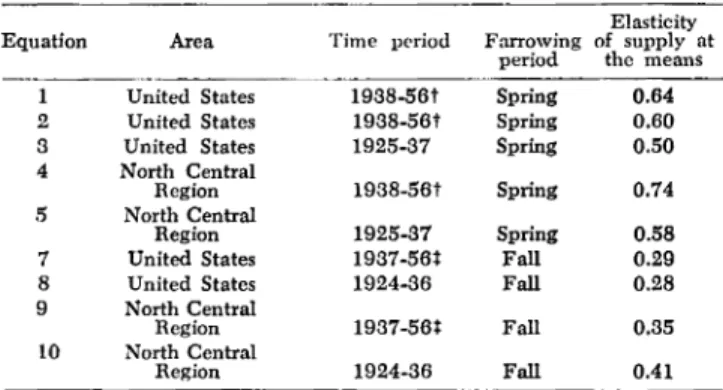
Single-equation least-squares methods were em-ployed in analyzing spring and fall farrowings in the United States and North Central Region for the periods 1924-37 and 1938-56. Factors which appeared important in explaining spring farrowings were (in order of importance) the hog-corn price ratio at breed-ing time, production of oats, barley and grain sorghum as a percentage of corn production in the previous year, and various measures of the relative profit-ability of hogs and beef cattle at breeding time. Co-efficients of determination (R2 values) of 0.90 or great-er wgreat-ere obtained for all spring farrowing equations. Estimated elasticities of supply (i.e., changes in far-rowings in response to hog prices at breeding time) for the United States increased from 0.50 in the
1924-572
37 period to about 0.62 in the 1938-56 period. For the North Central Region, the corresponding increase in supply elasticity was from 0.58 to 0.74. Hence, these results support the hypothesis of an increase in supply elasticity for hogs over time.
Factors which significantly influenced fall farrow-ings were the number of sows farrowing in the spring, production of oats, barley and grain sorghum, and the comparative profitability of hogs and beef cattle. Coefficients of determination (R2 values) were con-siderably lower for fall farrowings than for the spring farrowings. The supply elasticities for fall farrowings were relatively low (between 0.28 and 0.41) and did not change appreciably over time.
Estimates of supply elasticities also were obtained using an expected price model. Again, the response in spring farrowings to changes in hog prices expected in the future marketing period increased over time. The magnitudes of the elasticities computed from expected prices were comparable to those computed with respect to hog prices at breeding time.
In addition to changes in hog numbers, total hog supplies vary somewhat from changes in marketing weights. Simple three-equation simultaneous-equation models were used in estimating the responsiveness of farmers to price during 6-month marketing periods (i.e., by varying marketing weights). The within-mar-keting-period supply elasticities derived from this model were, as expected, relatively low-between 0.04
and 0.08; no appreciable changes occurred over time. Price and income elasticities of demand computed from the three-equation model showed a sharp de-crease from the 1924-37 to the 1938-56 period. While the magnitudes of the changes over time probably are overestimated by this model, the direction of change is consistent with the hypotheses advanced. In summary, the study provided support for the hypothesis of an increase over time in the supply elasticity for hogs, at least with regard to the number of sows farrowing in response to hog prices at breed-ing time. A decrease in the demand elasticity for hogs over time also was estimated. Therefore, recent observed wide fluctuations in hog prices may be explained, in part, by both an increase in the supply elasticity and a decrease in the demand elasticity for hogs.
Changes in Supply Functions and Supply
Elasticities in Hog Production!
BY GERALD W. DEAN AND EARL O. HEADY
A knowledge of supply responses and relationships for individual and aggregate agricultural commodities is of importance for farmers, economists, marketing organizations, national fann program administrators and consumers. Supply relationships are of immediate concern to outlook workers and other agricultural specialists who furnish information on which farmers base decisions. With more perfect knowledge, farmers might organize their resources for greater individual profits. A knowledge of supply functions would allow marketing firms to anticipate more accurately the timing and magnitude of future commodity supplies, leading to marketing efficiencies and lower consumer prices. Agricultural supply relations and elasticities also are vital for policy decisions, particularly those dealing with production control programs and price support levels for various farm products.
While many descriptive theoretical formulations of supply response are available in the literature rela-tively little research effort has been directed
t~ward
obtaining empirical estimates of supply relationships. Agricultural price analysts have concentrated heavily on the demand function for farm products, making the convenient assumption that the quantity supplied may be regarded as predetermined. For many farm commodities such a procedure has resulted in useful short-run predictions of price. Yet, more knowledge on the supply side is required if reasonably accurate representations of structural demand-supply interre-lationships are to be obtained.Pioneering work in the field of supply analysis began in the 1920's.2 The usual statistical technique employed in early supply studies was multiple re-gression, often by the short-cut graphic method. These analyses were hampered by the fact that the data were inadequate both in accuracy and in the period of time covered. As a result, the forecasts and relationships derived were frequently found misleading, and supply analysis generally fell into disrepute in the 1930·s.
1 Proiect 1135, Iowa Agricultural and Home Economics Experiment Station, Center for Agricultural Rnd Economic Adjustment cooperating. • For examples of some early contributions in supply analysis See: Bean, L. H. The farmers' response to price. Jour. Farm Econ. 11: 368-385. 1929.
Elliott, F. F. Adjusting hog production to market demand. III. (Urbana) Agr. Exp. Sta. Bu!. 293. 1927.
Wells, O. V. Farmers' response to price in hog production and market-ing. U. S. Dept. Agr. Tech. Bu!. 359. 34:1933.
Only since World War II has interest again revived in empirical supply studies.s
Price instability for several farm products has led to a further interest in supply phenomena. The hog ?larket, in particular, has shown wide price swings
III the rast several years. One measure of the
varia-bility 0 prices is the coefficient of variation (C). Table ~ indicates that in the months of heaviest hog market-mgs (October through April), year-to-year variations in deflated hog prices increased in the postwar period compared with the prewar period.
In the prewar period, data for 1931-34 were omitted because of the abnormally depressed hog prices throughout these years. From the prewar to the postwar period, the coefficient of variation increased from 16 percent to 25 percent, while in the 4 years 1953-57 the coefficient reached a high of 28 percent. The coefficient of variation for May through Septem-ber (the remaining marketing months) showed no change from the prewar to postwar period. Again, however, greater variability occurred in the 4 years 1953-57, as is evidenced by an increase in the C value to 21 percent. Many farmers, economists and legis-lators were especially puzzled by the low hog prices ~n the fall and winter of 1955-56. The present study IS an attempt to test hypotheses explaining the recent increased price fluctuations in the hog market. "Several recent empirical supply studies are:
Kohls, R. L. and Paarlberg, D. The short time response of agricultural
l~~~ction to price and other factors. Purdue Agr. Exp. Sta. Bul. 555. Halvorson, Harlow W. The supply elasticity for milk in the short run. Jour. Farm Econ. 37:1186-1197. 1955.
Bowlen, B. J. The wheat supply function. Jour. Farm Econ
37'1177-1185. 1955. . •
TABLE 1. MEASURE OF YEAR-TO-YEAR VARIATION IN DE-FLATED UNITED STATES HOG PRICES FOR SELECTED MARKET-ING MONTHS AND GROUPS OF YEARS.o
Marketing Standard Coefficients of Years months deviation Mean variation
•
(s) (x) (C=100:-) x 1923-42t October-April (dollars/cwt. ) (dollars/cwt. ) (percent) 2.34 14.64 16 1946-57 October-April 4.56 18.10 25 1953-57 October-April 4.36 15.53 28 1923-4H May-September 2.73 15.16 18 1946-56 May-September 3.43 19.49 18 1953-56 May-September 3.60 17.32 21
-o H-og prices deflated hy the Index -of Wh-ol ... ale P-;ces.
t Omitting three depression years from October 1931 to April 1934 ~ Omitting three depression years 1932-34. •
ECONOMIC THEORY
The "cobweb theorem" provides the basic theor-etical framework for the empirical results to be pre-sented.4 Briefly, the cobweb theorem is an attempt
to explai!1 recurring. cycles in the. J?roductio~ . and price senes for partIcular commodItIes .. Tradl~l?nal
economic theory assumes that, under statIc condItIons of pure competition, market price tends to be estab-lished at the intersection of the demand and supply curves. However, where a considerable time lag occurs between the price change for a commodity and the resulting supply response, the cobweb relationship may lead to widely fluctuating prices and quantities. Three possible cases of the cobweb theorem are distinguished:
Case 1. Continuous fluctuation. This case is
repre-sented geometrically by the left diagram in fig. 1. Assume quantity QI is produced in time period 1 and placed upon the market. The resulting price is estab-lished at Pl. However, the low price PI results in supply of only Q2 in time period 2. With only Q2 sup-plied, price is established at the relatively higl;t price P2. Producers respond to the price P2 by producmg Qs. But with the quantity Qa supplied, price once. more falls to Pa. Price Pa is the same as the original pnce Ph and the pattern then is repeated in following time periods. When the demand curve is the exact reverse of the supply curve (i.e., when the two curves have identical slopes at any chosen price) this same pattern theoretically will repeat indefinitely. Thus, in. the simple case of linear demand and supply ~unctIons, the continuous case occurs when both functIons have the same absolute slope.
Case 2. Divergent fluctuation. This case,
repre-sented by the center diagram in fig. 1, occurs when • Fot an excellent summary of the cobweb theorem see: Ezekiel, Mor-decai. The cobweb theorem. Quart. Jour. Econ. 52:255-280. 1938.
p p.
o
s
o
01
the absolute slope of the demand function is greater than that of the supply func:tion. ~eginning with. a quantity QI and correspondmg pnce PI the senes of reactions trace out a pattern of successively larger fluctuations in price and quantity.
Case 8. Convergent fluctuation. The right diagram
in fig. 1 represents the case of sucessively converging prices and quantities. Starting from quantity QI and price PI the quantities and prices show succ~s~ively
smaller fluctuations as they approach the eqUlhbrum point at the intersection of the demand and supply functions. In this situation the absolute slope of the supply function is greater than that of the demand function.
Three conditions are required for the cobweb theory to explain the functioning of a commodity market: (a) Producers must base output in per~od
t+l entirely on prices in period t; (b) productIon plans, once made, cannot be changed until the. fol-lowing time period; (c) price must be determmed by the quantity supplied. It appears that the demand and supply structure for hogs ~~ the Un~ted Stat~s approximately meets the Co~dlbons outlmed. It ~s
necessary, however, to investIgate each of th~ condI-tions in detail as it pertains to hog productIon and marketing.
In regard to condition (a), a few empirical .results are available which indicate the nature of pnce ex-pectation models used by fa~ers. Howeve.r, th~ pres-ence of commodity cycles m themselves IS eVIdpres-ence that many farmers use current prices as the basis for projection or forecasting. In one of the few em-pirical studies available, Schultz and Brownlee5
con-cluded that Iowa farmers formulated price expecta-tions for hogs largely on the basis of current prices, at least for the time period investigated. A more • Schultz T. W. and Brownlee. O. H. Two trials to determine ex-pectation' models applicable to agriculture. Quart. Jour. Econ. 56: 487-496. 1942. 01
o
01 CASE I Q0
01 CASE 2o
o
CASE 3 CONVERGENT FLUCTUATION Q CONTINUOUS FLUCTUATION DIVERGENT FLUCTUATION Fig ..1:
'Natfuce of' lllictuatioi1( iri -price and produ,ction under specified elasticity situations.realistic hypothesis is that farmers' price expectations are based not only on the current price but also on prices observed in previous years. The most recent price, however, probably carries the greatest influence, while the weight attached to each previous price declines as the time lag increases. On the basis of the rather limited evidence available, the first condition for a cobweb relationship in hog production (i.e., that farmers base price expectations on current prices) seems approximately satisfied.
The nature of the hog production process indicates that conditions (b) and (c) also are reasonably ful-filled. Once sows are bred for farrowing, relatively little can be done to increase future production. Great-er effort might be directed toward saving more pigs per litter, and hogs can be carried. to slightly heavier marketing weights, but these adjustments affect total supplies to only a relatively small extent. Somewhat greater flexibility is available in reducing supplies, since bred gilts may be sold before farrowing. Heavy price discounts on "piggy" sows, however, tend to minimize this possibility, at least after the second month of pregnancy. A more serious limitation in applying the cobweb theory to hog production may be that hog supplies depend heavily on corn prices as well as on hog prices. However, hog prices in the heaviest marketing period of late fall and winter reflect, in part, the new corn supply and hence the expected price of corn during the next year. Condition
18.0
0
11 .0 lJJa
16.0 cz
<tP35
03S
;> 15.0...---+----i--.
o
z ~14.0 t-= (.) 0 13 .0 z 912.0~
Q~7(c) implies no interdependence or simultaneity be-tween the price received and the quantity supplied; i.e., quantity is assumed to be predetermined. While farmers do vary marketing weights in response to short-run price changes, the resulting influence in the total hog supply picture probably is relatively minor.
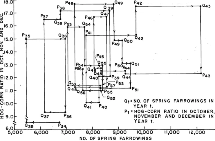
The above discussion suggests the possibility of a cobweb pattern of price and production in the United States hog market. Further evidence of this relation-ship is provided in fig. 2, where the hog-corn price ratio in October, November and December is measur-ed along the vertical axis, and the number of spring farrowings (in units of 1,000 sows) is measured along the horizontal axis. Since the corn supply is a major factor in hog production, hog-corn price ratios, rather than hog prices alone, are used in fig. 2. October, November and December are the main months in which sows are bred for spring farrowings. The gesta-tion period for hogs is approximately 4 months, while the feeding period required to raise hogs to market weight is another 6 to 8 months. Hence, the pigs raised from sows bred one fall usually are sold the next fall, some 10 to 12 months later. The prices at which hogs of the previous spring pig crop are market-ed then are known prior to bremarket-eding time for the next spring pig crop. If the cobweb theorem is alii. accurate description of the hog market, relatively high hog prices one fall would lead to a large
num-P42-
Q ~---~~43
a: zll.O a:o
010.0048056
'\ PSIS
PSI
I \...052
at:; NO. OF SPRING FARROWINGS IN
I t!)
o
YEAR
t.
Pt
=
HOG-CORN RATIO IN OCTOBER,NOVEMBER AND DECEMBER IN
x
9.0 ~. . o { . YEAR
t.
6.01~~_0~3~5~~I~
____
P~3~4~'~~
__
~~~
____
~~=-
__
~~I~~
__
~~I~~
__
~~I~~
___
5,000 6,000 7,000 8,000 9,000 10,000 '1,000 12,000
NO. OF SPRING FARROWINGS
Fig. 2. Relation of hog fnrrowings and hog prices, 1934-56.
ber of farrowings the next spring. Pigs from this large spring crop would be marketed the following fall, driving hog prices downward. Low hog prices would induce a smaller number of spring farrowings, which in turn would lead to higher hog prices the following fall, etc.
Figure 2 proVides strong indications that, with some modification, such a process has in fact taken place in the United States. The low hog-com price ratio in the fall of 1934 (P34 ) induced only 5,467,000
spring farrowings in the spring of 1935 (Q35)' This low number of spring farrowings resulted in a short supply in the fall of 1935 and a relatively high hog-com price ratio (PaG). The higher hog-com ratio (P35 )
en-couraged a larger number of spring farrowings in
1936 (Q;w), which, in tum, resulted in a lower
hog-com ratio (P3G) in the fall, etc. There is sufficient regularity in the clockwise rotation to indicate an underlying cobweb relationship. At times the pattern appears to be shifted out of its regular course by some outside force. For example, the effects of World War II and the Korean conflict seem to disrupt the regularity of the cobweb pattern. Of course, other factors, such as the quantity of small grain production and the prices of competing farm products, undoubt-edly play a role not accounted for by this simple model. Nevertheless, it is suggested that the cobweb relationship is the appropriate theoretical framework for explaining price and quantity fluctuations in the hog market of the United States.
HYPOTHESES AND OBJECTIVES
The major hypothesis advanced in this investigation is that part of the recent fluctuations in hog prices can be traced to shifts in the supply elasticity for hogs. Specifically, it is hypothesized that the elasticity of supply for hogs has increased in recent years. As illustrated by the cobweb theory, an increase in supply elasticity (a flattening of the supply curve) leads to wider price fluctuations, other things remaining equal. Of course, an increase in supply elasticity does not necessarily mean that the hog market will be char-acterized by increasingly wider fluctuations. Starting from the convergent case, an increase in supply elastic-ity might not cause a shift to the continuous or diverg-ent fluctuation cases; the relationship of the demand and supply curves still could fall well within the con-vergent case, with only the convergence delayed. A secondary hypothesis is that the demand for hogs has become more inelastic in the past few years. Under the cobweb hypothesis, a demand curve with greater absolute slope than formerly also could lead to wider fluctuations in hog prices. It is hypothesized that the combination of these two forces-increased supply elastiCity and decreased demand elasticity-explains in part the recent behavior of the hog market.
It is fairly obvious that the production function for hogs has shifted upward in recent years, causing a corresponding downward shift in the marginal cost curve (assuming prices of inputs constant). Use of improved feeding, breeding and management practices now allows greater output per unit of resource input than was possible a few years ago. However, there .576
is no a priori reason why this shift in the production function should cause a shift toward greater elasticity in the marginal cost curve, and hence in the supply function. While the marginal cost curve is shifted down and to the right, making it appear flatter, elasticity (a percentage change concept) may remain constant or even decrease. Yet, an appraisal of changes in the farm economy suggests the plausibility of an increase in the supply elasticity for hogs in recent years. The hypothesis of increased supply elasticity for hogs implies that farmers are in a position of increased flexibility with respect to hog production. That is, producers now can shift more readily be-tween enterprises with the occurrence of relative price changes. Improvements in building facilities and equipment, as well as in technical managerial skills, have made possible this type of between-enterprise flexibility. Changes in pork production methods also might contribute toward increases in supply elasticity. The time required to raise hogs to market weight has shortened in recent years, be-cause of widespread adoption of new advances in swine nutrition, breeding and sanitation. Thus the impacts of price changes are felt more rapidly in increases or decreases in output. Also, some producers now use a multiple-farrowing system where pigs may be farrowed several times each year, or in some cases during every month of the year. Such a farrow-ing scheme allows much greater intra-year output adjustment to price changes than is possible under a rigid one- or two-litter-per-year system.
The reasoning behind the hypothesis of a lower demand elasticity for hogs lies in changes in con-sumer preferences for meat. ShepherdG et al have
shown an upward shift in the demand curve for beef and a downward shift in the demand curve for pork over time. In recent years pork apparently has be-come a less acceptable substitute for beef, poultry and other products.
The objectives of the study How directly from the hypotheses outlined above. A main objective is to empirically test the hypotheses of changes in supply and demand elasticities over time. Evidence on the directional shifts in elasticity was obtained, as well as point estimates of the magnitudes of these elasticities. Also, forecasting equations were de-veloped to predict hog supplies in future time periods. Since the demand-supply relationships for hogs are not independent of other livestock products, auxiliary information is presented regarding these other pro-ducts.
CHOICE OF ESTIMATIONAL PROCEDURES A number of alternative procedures are available for deriving supply relationships in agricultural pro-duction. One general classification of procedures deals with the supply response of individual "typical" farm finns. Survey data from a sample of fanns may pro-vide information on the factors influencing supply • Shepherd, G. S., Purcell. J. C. and Manderscheid. L. V. Economic analysis of trends in beef cattle and hog prices. Iowa Agr. Exp. Sta. Res. Bu!. 405. 1954 .
response; such dat~)illso may reveal past and antici-pated changes in production in response to price and other phenomena. Another method of estimating supply response is to determine the optimum pattern of farm production for various price relationships. The technique of linear programming has increased the feasibility of this approach in recent years.7 Still
another approach at the firm level is the study of the production function and related cost curves. A major difficulty in all firm approaches, however, is the problem of aggregating firm supply functions into an industry supply function.
Another group of procedures attempts to estimate the aggregate supply function directly, usually from annual, quarterly, monthly or daily time series data. One problem encountered in the aggregate approach is that individual firm adjustments, which may offset or cancel one another, tend to be obscured. A second problem lies in the choice of appropriate statistical techniques in analyzing time series data. Nevertheless, the aggregate method is used in this study because primary interest is in aggregate relationships.
Since the present study employs statistical analysis of time series data, the question arises: Should single-equation least-squares methods be used, or are simul-taneous equations appropriate? The appropriate me-thod of statistical estimation is determined by the degree of identification of the equations in the model.
It is impossible to derive unique estimates of the coefficients of an equation which is under-identified. \Vhen an equation is just-identified, the coefficients can be estimated by an indirect use of least squares. In this case, it is possible to make two simple unique transformations. One transforms stmctural equations into reduced-form equations, each containing one endogenous variable, which can be estimated by least squares; the other transforms the least-squares esti-mates of the coefficients back to estiesti-mates of the structural coefficients. Because of its simplicity, this method has been used in most applications of simul-taneous equations. When an equation is over-identi-fied, more difficult problems of statistical estimation arise. Theoretically, the ideal method for obtaining structural coefficients in this case is the maximum-likelihood method. The maximum-maximum-likelihood pro-cedure provides a means of arriving at a reconciliation of the finite number of alternative estimates obtained in the over-identified situation. Logically, the "full-information" maximum likelihood method, which utilizes all of the information in the model, is considered superior for the estimation of over-identified equations. However, this procedure is formidable from a computational standpoint. Hence, the "limited-information" maximum-likelihood method, which utilizes only part of the available information, is employed in this study for the estimation of over-identified equations. Details of the computational procedure followed are set forth by Friedman and Foote8 and are summarized in matrix notation by
Chernoff and Divinsky.9
7 See Heady, Earl O. mld Candler, W. V. Linear progranuning methods. Iowa State University Press, Ames. 1958.
• Friedman, Joan and Foote, R. J. Computatinnal methods for handling Nystems of equations. U. S. Dept. Agr. Handb. 94. 1955.
,. Chernoff, Herman and Divinsky, N. The computation of maximum-likelihood estimates of linear structural equations. In Cowles Commis-sion for lIesearch in Economics. Monograph 14: 236-269. Jobn Wiley and Sons, New York, N. Y. 1953.
ANALYSIS OF SPRING AND FALL HOG FARROWINGS IN THE UNITED STATES
AND NORTH CENTRAL REGION
The total liveweight production of hogs in the United States depends directly, upon the number of hogs marketed and their average marketing weight. For reasons mentioned earlier, average marketing weights vary relatively little from year to year; the major changes in hog supplies result from changes in the number of hogs marketed. The number of hogs marketed is, in turn, determined largely by the num-ber of sows which farrowed in preceding time periods. Thus, the first and perhaps most important step in studying hog supply is an analysis of spring and fall farrowings. The analysis is carried out at two levels of aggregation: One analysis pertains to the United States as a whole; the other relates to the North Central Region. Since, depending on the year, 70 to 80 percent of the spring pig crop (December through May) and 60 to 70 percent of the fall pig crop (June through September) are produced in the 12-state North Central Region, this area is singled out for special study.
To investigate the hypothesis of an increased supply elasticity for hogs, the analysis is further divided into two time periods. Comparisons between these time periods provide estimates of changes in structural relations. A logical division with respect to time might be into prewar and postwar periods. Most available agricultural demand analyses are based on the interwar period from about 1920 to 1941. A few analyses include several postwar years along with the prewar period, omitting the war years because of disturbances due to government interference in pric-ing, rationpric-ing, etcY' In the latter procedure, how-ever, changes in structural relationships over time may be obscured. On the other hand, a separate post-war analysis must be based on rather scanty data. As a compromise, the time periods selected for study are 1924-37 and 1938-56 (omitting war years 1942, 1943 and 1944). In terms of relatively homogeneous periods, this appears to be a reasonable division. By 1938 the United States had recovered from the depths of the depression. Also, the agricultural sector no longer felt the major effects of the drouth years 1934 and 1936.
The nature of the production process for hogs indicates that a single-equation least-squares model is appropriate in estimating spring and fall farrowings. Because of the 4-month gestation period for hogs, the number of sows farrowing cannot be changed quickly in response to price clianges during the far-rowing period. Most producer decisions regarding the number of sows to farrow are made at or before breeding time, preceding the farrowing period. There-fore, numbers of sows farrOWing may be regarded as a function of predetermined variables, known in
advance of the farrowing months. Two qualifications should be noted: First, since the farrowing periods
10 The reasons for omitting the war years in the supply analysis are less apparent, since producers supposedly react to market prices whether they are administered or not. Howcver, in this part of the study, the "arlier war years are omitted because increased wartime production may have resulted from patriotic motivations, etc., rather than from response
to rnpa.~urab]e phenomena.
are defined as 6 months in length and the gestation period is only 4 months, prices at the beginning of the period might influence the number of farrowings at the end of the period. Second, bred sows may be sold during the gestation period if the outlook is for unfavorable hog prices. These factors, while recog-nized, are believed to be of insufficient importance to destroy the assumption that farrowings are essen-tially predetermined.
SPRING FARROWINGS IN THE UNITED STATES
Regression equations 1 and 2 estimate spring far-rowings in the United States for the period 1938 to 1956 (omitting war years 1942, 1943 and 1944). Stand-ard errors of the regression coefficients are given in parentheses below the coefficients.
(1) '£'
=
-5,970+
392X1+
60X2 - 105X3(34) (11) (54)
'£'
=
-7,430-I-
418X1+
66X2+
578X4(36) (11) (229)
(2)
The variables are defined as follows:
R2=0.92 d =1.55 R2=0.93 d =1.02
Y :::: Estimated first difference in the number of spring far-rowings, United States (in 1,000 litters). The spring far-rowing period extends from December, year t-l, through May, year t.
X,:::: United States hog-com price ratio as an average of October, November and December, year t-l; computed as the ratio of average hog prices in dollars per hundred-weight to average com prices in dollars per bushel. X,:::: First difference of oats, barley and grain sorghum
pro-duction as a percentage of com prodUction, United States. That is, St-1 - St_., where S denotes oats, barley and grain sorghum production as a percentage of com production (production in tons). This variable is coded by adding a constant of 15.0 to remove negative values. X,:::: Margin or difference between the average price (in dollars per hundredweight) of 500-800 pound good-choice stocker and feeder cattle at Omaha and the average price (in dollars per hundredweight) of chOice-prime slaughter steers of all weights at Chicago during October, Novem-ber and DecemNovem-ber, year t-l, deflated by the Index of Wholesale Prices (1910-14 :::: 100).
X. :::: Ratio between the average price (in dollars per hundred-weight) of 500-800 pound good-choice stocker and feeder cattle at Omaha and the average United States hog price (in dollars per hundredweight) during October, November and December, year t-I.
In both equations, the hog-corn price ratio (Xl) is the most important variable in predicting changes in spring farrowings, as judged by the standard partial regression coefficients. It appears that the absolute level of this ratio strongly influences the direction and magnitude of changes in farrowings. When hog prices are favorable relative to corn (a high hog-corn price ratio), farrowings tend to increase from the previous level and vice versa.
The hog-corn ratio reflects to a considerable extent the supply of corn available for feeding. However, Brandowl l notes a separate influence on hog supplies exerted by the production of oats, barley and grain sorghum. When these grains comprise a relatively
11 Brandow, G. E. Factors associated with numbers of sows farrowing
in the spring and fall seasons. Pa. ,\gr. Exp. Sta. A. E. and R. S. 7, 1956. 578
large proportion of the total feed grain supply, hog production tends to increase and vice versa. The variable expressing this relationship (X2) is next in importance in explaining changes in spring farrow-ings.
Beef cattle feeding probably is the chief competitive farm enterprise with hogs in the major hog-raising areas. According to theory, the relative profitability of cattle and hogs should influence the number of sows farrowing. The third variables in equations 1 and 2 represent two possible methods of expressing this influence. The regression coefficient for the de-flated price margin on beef cattle (X3) is negative,
indicating that as margins increase, the number of sows farrowing the following spring decreases and vice versa. For example, when cattle margins are relatively high, resources apparently are shifted from hog production to beef cattle production. In equation 2, the price ratio between feeder cattle and hogs (X4)
indicates the relative attractiveness of beef cattle versus hog production. When feeder cattle prices are relatively high, farmers tend to reduce cattle pro-duction and increase hog propro-duction. l2
Figures 3 and 4 show the actual spring farrowings compared with those predicted from equations 1 and 2. Admittedly, comparing the predicted and actual farrowings over the time period used in developing the regression equation is not a completely satisfactory test of the value of the equation for predictional pur-poses.l3 Recognizing the limitations of this test, the
regression equations correctly indicate the direction of change in spring hog farrowings, with the single exception of the 1945 prediction for 1946 in fig. 3. Some idea of the precision of the estimates is given by computing the standard error of the esti-mate. This figure provides a measure of the amount by which the estimates of farrowings deviate from the observed farrowings in the years studied. For equation 1, the standard error of the estimate is 275,000 litters or approximately 3.36 percent of the mean number of farrowings each spring. Of course, the standard error of a forecast is somewhat larger. The standard error of the estimate for equation 2 is 256,000 litters or 3.13 percent of the mean number of sow farrowings.
The Durbin-Watson14 test for serial independence of the residuals also is computed, although the rela-tively low number of observations increases the
prob-12 While not shown here, a slaughter cattle-hog price ratio is nearly
as effective as the feeder cattle-hog price ratio in predicting changes in sows farrowing. Because of the high correlation between feeder cattle Wld slaughter cattle prices, Il,e regression coefficient for the slaughter cattle-hog price ratio also has a negative sign. This result appears in-consistent with logic. In almost all the analyses undertaken. some fonn of beef cattle-hog price ratio is Significant; however, the signs are sometimes positive, sometimes negative. Since feeder and slaughter cattle prices are highly correlated, either a feeder cattle-hog ratio or slaughter cattle-hog ratio prodoces a significant regression coefficient. Thus, it is possible to argue that producers are influenced in some instances by feeder cattle prices and in others by slaughter cattle prices. While it is always possible to obtain a "consistent" sign in this way. the method appears highly arbitrary. More investigation is needed on this re-lationship.
13 A somewhat better test might be to test one year at a time. For
example, the data for 1938-55 could be used to develop a regression equation containing the same variables used in equations 1 and 2. Then, an estimate for 1956 could be made and compared with the actual 1956 value. This could be done, however, for only a few recent years in the time series .
.. Durbin, J. and Watson, G. S. Testing for serial correlation in least-squares regression II. Biometrica. 38:159-178. 1951.
o CI 10.0 9.0 uJ :I: " \ \ , 'I; \ \ \ - - - ACTUAL - - - - PREDICTED
pll~ __ ~~I ______ -LI ______ ~I~ ____ -JI~ ____ ~I~~~~1
·'="---:-::19:'-::4:-::0:-O-':-:19:-"4:-::2-:!1fI944 1946 1948 1950 1952 1954· 1956
Fig. 3. Actual spring farrowings In the United States compared with predictions from equation 1.
o CI UJ :I: 10.0 9.0
--
/~ '/ '\ fi' \ \ \ ---ACTUAL - - - - PREDICTED ~~--~19~4~0--~19~4~2~IPI~:-4~4~--~19~~~6---19L~-8---1-9LI5-0--~-I~~~52---19J'5-4----1-9~5~Fig. 4. Actual spring farrowings in the United States compared with predictions based on equation 2.
ability of obtaining an inconclusive test result. The d statistic for equation 1 is 1.55, which falls in the inconclusive range. However, the d statistic for equa-tion 2 is 1.02, indicating that the hypothesis of serial independence in the residuals is rejected. When plotted, the residuals for equation 2 show a slight cyclical effect, probably accounting for the signifi-cant test result.
Regression equation 3 is computed for spring far-rowings in the United States during the earlier period, 1924-37. Variables t, Xl and X2 are the same as those
defined earlier. Variable Xa is similar to Xs; it is the average price margin (in dollars per cwt.) between (3) t = -7,401
+
366X1+
28X2+
962X5 R2=0.92(35) (10) (249) d =1.42 feeder cattle and slaughter cattle prices at Chicago from August to December, year t-l, deBated by the Index of Wholesale Prices (1910-14=100). Chicago feeder cattle prices are used because the Omaha series
does not extend back to 1924. However, the sign of the regression coefficient is positive for Xli, the op-posite of Xa in equation 1. Economic logic indicates that as cattle margins increase, making cattle pro-duction more favorable, hog propro-duction should de-crease. Perhaps in the earlier time period cattle mar-gins were viewed more as an indicator of profit-ability of livestock production in general, rather than in a strictly competitive role with hogs. The extended depression period might have contributed to such psychology on the part of producers. A more likely explanation is that, when margins are high, feeder cattle prices also are usually high, discouraging beef cattle production. Again, more study is needed of the supply interrelationships between beef cattle and hogs.
As shown in fig. 5, regression equation 3 indicates the correct direction of change in hog farrowings in every year. The standard error of the estimate for equation 3 is slightly larger than those for the later time period - 355,000 litters per year or about 4.11 579
10.0 9.0 o ~8.0 :r:
z
o -.J ~7.0 ~ 6.0 ---ACTUAL - - - - PREDICTED 5.0~_---:-="=,=---....,-,,I,=,,---:-::-I::-:::---,.I:~----:~--=':::-=---:-=".=7-1924 1926 1934 1936 1938Fi~. 5. ActulIl sprin~ farrowin~s in the United States compared with lltcdictiullS ha,,'" IlIl I''1"ution 3.
percent of the mean number of farrowings. The Durbin-Watson d statistic is 1.42, again an incon-clusive test result.
SPRING F AHROWINGS IN THE NORTH CENTRAL REGION As mentioned previously, 70 to 80 percent of the spring farrowings in the United States normally occur in the 12-state North Central Region.lli Because of the importance of the North Central Region in the total hog supply picture, regression equations 4 and 5 are computed for this region alone, for the two periods 1938-56 (omitting years 1942, 1943 and 1944) and 1924-37, respectively.
(4) t
=
-6,770+
400X1+
50X:!+
726Xu R2=0.93(33) (9) (195) d =2.01 (5) t
=
-6,621+
316X1+
22X2+
894X7(35) (10) (248) The variables are defined as follows:
Y = Estimated first difference in the number of spring far-rowings, North Central Region (in 1,000 litters). The spring farrOWing period extends from December, year t-1, through May, year t.
XI = Chicago hog-corn price ratio as an average of October. November and December, year t-1; computed as the ratio of average hog prices in dollars per hundredweight to average corn prices in dollars per bushel.
X. = As defined previously.
X. = Ratio between the average price (in dollars per hundred-weight) of 500-800 pound good-choice stocker and feeder cattle at Omaha and average Chicago hog price (in dollars per hundredweight) during October, November and December, year t-1.
.. The state. included ill this r~gion are: Ohio, Indiana, Illinois, Michigan, Wisconsin, Minnesota, Iowa, Missouri, North Dakota, South Dakota. Nebraska and Kansas.
580
X. = Margin or difference between the average prices (in dollars per hundredweight) of all feeder cattle and slaughter cattle at Chicago as an average for the months August through December of year t-1, deflated by the Index of Wholesale Prices (1910-14=100). ,
In equation 4 for the later time period, the hog-corn ratio (Xl) remains the most important explan-atory variable, followed by X2 and Xo, respectively.
Once again the coefficient for variable Xo (the feeder cattle-hog price ratio) is positive and 3.73 times as large as its standard error.lO Figure 6 shows the actual farrowings for the North Central Region compared with those predicted by equation 4. The direction of yearly changes is predicted correctly for every year except 1946. Regression equation 1 for United States spring farrowings also failed for this year (see fig. 3). The standard error of the estimate for regression equation 4 is 199,000 litters per year or approximately 3.20 percent of the mean number of
spring farrowings in the North Central Region. The calculated value of the Durbin-Watson d statistic is 2.01, indicating support for the assumption of serial independence of the residuals.
The coefficients of equation 5 for the North Central Region (1924-37) are similar to those obtained in equation 3 for the United States. Again, X1 (de-flated cattle margins), while large relative to its standard error, has a sign inconsistent with economic logic. Figure 7 shows that regression equation 5 cor-rectly indicates the direction of change in farrowings for every year. The regression equation for 1924-37 again has a larger standard error of the estimate than the equations for 1938-56. The standard error of the ,. As pointed uut previously, the .laullhter cattle-holl price ratio is nearly as effective as the feeder cattle-hog price ratio in these equations. If interest is primarily in prediction rather than in estimation of structural relationships, some criterion such as the highest R2 value might be used in selectiog hetween these two variable •.
8.0 7.0 ---ACTUAL ' - - - - PREDICTED ~ \ \
,
~"
\ \ \ I I 1~42 1944 '1946 1948 , 1950 1952Fig. 6. Actual spring farrowings in the North Central Region compared with predictions based 011 ~qu"lioll 4.
9.0
B.O
o c:t7.O UJ X Zo
:i6.0 ...J :!: 5.0 ---ACTUAL - - - - PREDICTED 4.0 1924 1932.i 1938Fig. 7. Actual spring farrowing. in the North Central Region compared with prl'dictiolls bn,,'d 011 {''1mllion ,5.
estimate for equation 5 is 332,000 litters per year or 5.20 percent of the mean number of spring farrowings in the North Central Region from 1924-37. The Dur-bin-Watson d statistic for equation 5 is 1.75, indicat-ing that the assumption of serial independence in the residuals is not rejected.
FALL FARROWlNGS IN THE UNITED STATES The fall farrowing period as defined by the United States Department of Agriculture extends from June 1 to Nov. 30. Regression equation 6 is compute for fall farrowings in the United States for the period 1937-56 (omitting years 1941, 1942, 1943 and 1944).
(6) '? = 159.91
+
0.29Xl+
0.7BX:!+
S.9BX:: (0.09) (1.99) (1.10)+
B.14X4 R:!=0.92 (2.62) d=
not computed (7) '?=
237.96+
O.28Xl+
4.ooXa+
B.46X4 R:!=0.92 (0.09) (1.06) (2.39) d =1.70 Regression equation 7 becomes the prediction equa-tion when variable X2 is dropped from equation 6.The variables in the equations are:
r
=
Estimated number of fall farrowings, United States (in 1,000 head). The fall farrowing period extends from June through November, year t.Xl
=
Number of spring farrowings, United States (in 1,000 head); i.e., from December, year t-1, through May, year t. X.=
United States hog-corn price ratio as an average ofMarch, April, May and June, year t; computed as the ratio of average hog prices in dollars per hundredweight to average corn prices in dollars per .bushel.
X, = Quantity of oats, barley and grain sorghum produced (in 100 tons), United States, year t.
X,
=
Ratio of the average price (in dollars per cwt.) of slaughter steers, all grades, at Chicago to the average price of corn (in dollars per bushel) at Chicago during March, April, May and June, year t.The hog-corn price ratio at breeding time (March, April, May and June) for fall farrowing has a non-significant regression coefficient in equation 6. Thus, while the hog-corn price ratio at breeding time is the most important variable influencing spring farrowings, the corresponding factor does not significantly influ-ence fall farrowings. More important than the hog-corn price ratio in determining fall farrowings are the number' of spring farrowings, anticipated feed grain supplies and the competitive position of hogs with cattle. Many producers plan during the fall months for production over the entire year' ahead. That is, plans are made for a certain number of sows to far-row in the spring, then the same sows are carried over and farrow again in the fall. Since many farmers follow this two-litter system, the number of fall farrowings apparently is influenced more by the hog-corn ratio in the previous fall than by this ratio at breeding time for fall pigs (March, April, May and June). In this situation, the decision to farrow sows for the fall period is a "routine" or "automatic" decision not appreciably influenced by prices at breeding time.
In fitting equation 7, the actual quantity of small grain production (X3 ) in year t was used. Of course,
the magnitude of this variable is quite uncertain at the time decisions are made to breed sows for early fall farrowings. As indicated above, however, this
6.0 5.5 5.0
..
z 0 :i -I 4.5 :!!decision often is made rather automatically. Later on, when more evidence is available on potential grain supplies and other factors, a portion of the bred sows may be sold. The practice of breeding sows, with the alternative of selling them before farrowing if conditions appear unfavorable, provides added flexi-bility under uncertainty and apparently is used by a number of hog producers. Forecasts from equation 7 probably would be made in June, at which time reasonably accurate estimates of the current year small grain production are available.
In equation 7 the relative profit position of beef cattle and hogs is expressed through a slaughter cattle-corn price ratio. According to equation 7, rela-tively high cattle prices at breeding time for fall pigs are associated with a greater number of fall far-rowings. Again, either a slaughter cattle-corn price ratio or a feeder cattle-corn price ratio is eHective in raising the R2 value in the regression equation for fall farrowings. Perhaps farmers are mainly influenced by feeder cattle prices. If so, a feeder cattle-corn ratio variable might be defended as follows: Pros-pectively high feeder cattle prices require a greater outlay and increase the risk associated with the beef cattle enterprise. Resources then are shifted into in-creased hog production. Conversely, when feeder cattle prices are relatively low, risk in cattle feeding is lessened and resources are diverted from hogs to cattle production.
Figure 8 compares the actual fall farrowings in tlle United States with the predicted farrowings from equation 7. With the exception of 1951, the pre-diction is in the correct direction in every year. The standard error of the estimate is 177,000 litters or 3.48 percent of the mean number of fall farrowings in the 1937-56 period. The calculated d statistic for equation 7 is 1.70. Once again the hypothesis of serial independence of the residuals is not rejected.
---ACTUAL - - - - PREDICTED ! . I 3.5 1938 1940'1944 1954 1956 1936 1946 1948 1950 1952
Fig. 8. Actual fall farrowings in the United States compared with predictions IlIls~d nn erluatin" 7.
5.5 5.0 o ~4.5 :I: z o ...I ...14.0 :E \ \ \ \ \ \ \ \ 3.5 - - - ~CTUAL \ \ \ \ \ - - - - PREDICTED '3.0 19~2~2----~19~2~4----~19~2~6----~~--~~~--~19~3~2~--~~--~~~
Fig. 9. Actual fall farrowing. in the United States compared with predictions based on ~qllation S.
Regression equation 8 is computed for fall farrow-ings in the United States, based on data for the period 1924-36. Variables t, Xl and X4 are defined
the same as for equations 6 and 7. Variable X5 expresses the influence of feed grain supplies; it is measured as the change in corn production (in 100-(8) t=369.13+ 0.29Xl + 1.38X5 + 11.55X4 R2=0.75
(0.08) (0.64) (4.13) d =2.45 ton units) from year t-l to year t. Again, the hog-com ratio at breeding time for fall farrowings (X2) has a nonsignificant regression coefficient and therefore has been excluded from equation 8. As shown by the R2 value of 0.75 the explanation of variance in the de-pendent variable (fall farrowings) by the chosen in-dependent variables is less satisfactory than in equa-tions 6 and 7 for the later 1937-56 period. Part of the explanation for this difficulty appears to be the uncertainty of, and wide fluctuations in, feed grain supplies during the later years of the 1924-36 period. For example, in fig. 9 large prediction errors occur in 1933, 1934 and 1936, years in which feed grain supplies shifted drastically from the level of the previous year. Also, regression equation 8 predicted the wrong direction in fall farrowings for the three years 1929, 1933 and 1936. The standard error of the estimate - 346,000 litters or 8.04 percent of the mean - is larger than in previous equations. The DurbWatson d statistic for equation 8 is 2.45, which in-dicates an inconclusive test result. If equation 11 were relevant for forecasting purposes, it would be desirable to refine it further. However, the purpose of studying the earlier time period (1924-36) is to estimate regression and elasticity coefficients for the important variables. Comparisons of supply elasticities computed from the regression equations are presented later.
FALL FARROWINGS IN THE NORTH CENTRAL REGION The 12-state North Central Region produces a somewhat smaller percentage of the total United States fall pig crop than of the spring pig crop; the percentage historically has been between 60 and 70 percent. From 1950-56, however, the percentage of total fall farrowings produced in the North Central Region has increased to between 70 and 75 percent. Regression equations 9 and 10 are computed for the 1937-56 (omitting 1941, 1942, 1943 and 1944) and 1924-36 periods, respectively.
(9) t= -941.89 + 0.23X5 + 5.46Xa + 8.20X~R2=0.89 (0.12) (1.39) (2.79) d =1.27 (10) t = - 390.11+0.32X5 +0.B4Xa + 8.51X4 R2=0.71 (0.05) (0.25) (4.03) d =2.50 The variables are defined as follows:
?
=
Estimated number of fall farrowings, North Central Region (in 1,000 head). The fall farrowing period extends from June through November, year t.X.
=
Number of spring farrowingsl North Central Region (in1,000 head) i.e., from Decemoer, year t-l, through May, year t.
X.
=
Quantity of oats, barley and grain sorghum produced (in 100 tons), United States, year t.X. = Ratio of the average price of slaughter steers, all grades, at Chicago to the average price of com (in dollars per bushel) at Chicago during March, April, May and June, year t.
X.
=
Change in com production (in 100 tons), United States, from year t-l to year t.The logic of the variables has been explained pre-viously and will not be repeated. Figures 10 and 11 show that the predictions for the 1937-56 period are more accurate, both in direction and in magnitude, than those for the 1924-36 period. Regression equation 583
4.5 4.0 0 <X 3.5 w :t: Z 2 --1 --1 3.0 :E 2.5 ... , I 'I V --ACTUAL - - - - PREDICTED \ \ \ \ \ \
Fig. 10. Actual fall farrowings in the North Central Region compared with prediction based on equation fl.
4.0 3.5 o <f IJJ 3.0 J: Z o ..J ;::!2.5 :i! - - ACTUAL 2.0 - - - - PREDICTED 1.5 '="="---;-;;;~----:-:-'~---;-;~;----:-::::'::=-=--""""7::'""="--~-:---=-=:~ 1922 1924 1926 1928 1930 1932
Fig:. 11. Actual fall faTrowings in the North Central Region compared with pn.-dictions hl.lsl'd Oil equation 10.
9 predicts the direction of change correctly in every year except 1940 (fig. 10), while equation 10 predicts the incorrect direction of change four times in the earlier 13-year period (fig. 11). Again, equation 10 is not further refined because interest in the earlier time period centers on measuring the influence of the major independent variables rather than on fore-casting. The comparative precision of equations 9 and 10 is revealed by their standard errors of mate. For equation 9, the standard error of the esti-mate is 204,600 litters or 7.0 percent of the mean number of fall farrowings in the North Central States. For equation 10, however, the standard error of the 584
estimate is 380,600 litters or 13.1 percent of the mean number of farrowings. The calculated d statistic for equation 9 is 1.27, which falls in the rejection region. That is, the hypothesis of serial independence in the residuals is rejected. For equation 10 the d value is 2.50, providing an inconclusive result.
ELASTICITIES OF SUPPLY FROM FARROWING EQUATIONS Elasticity of supply is defined as the percentage change in quantity associated with a I-percent change in price. Equation 11 gives the various mathematical formulas used in computing the elasticity of supply
(11) E _ Percentage change in quantity
S - Percentage change in price
L).Q P.
oQ
P X = X -L).P QoP
QaQ
P
In this study the last formula (--
X -)
is usedoP
Q
in computing elasticities. AU elasticities are evaluated at the means of the variables.
The supply elasticities presented below measure the percentage change in the number of farrowings associated with a I-percent change in the average hog price at breeding time. For spring farrowings t~e
supply elasticities measure the percentage change m number of farrowings (Q) from December, year t-l, through May, year t, associated with a I-percent change in average hog price (P) in October, November and December, year t-1; i.e., at breeding time for spring farrowings. However, a somewhat different procedure is used in computing supply elasticities for fall farrowings. Regression coefficients for hog prices in March, April, May and June, year t, are non-significant in predicting fall farrowings (from Jtme through November, year t); supply elasticities based on these coefficients would be rather meaningless. Hence as in the case of spring farrowings, elasticities for fali farrowings, year t, are computed with respect to average hog prices in October, November and December, year t-1. The rationale for this procedure
is that decisions are made in the fall, year t-1, appar-ently for both spring and fall farrowings, year t.
Computational details of this procedure are presented later.
An example of computing the supply elasti~ity
for spring farrowings is given next for regresslOn equation 1. Variable t is the estimated year-to-year change in spring farrowings; i.e., t
=
(tt -
Yt-
1).Variable Xl is the hog-corn ratio in the previous fall; i.e.,
Price of hogs Ph
Xl
=
Thus, equation 1 mayPrice of corn Pc
be rewritten as equation 12. The partial derivative
ott
of quantity with respect to hog price - - - is given
oP
hin equation 13. The definition of elasticity of supply (1)
t
= -
5,970+
392Xl+
60X2 - 105X3 Ph (12)tt -
Yt .l =-5,970+
3 9 2 - + 60X2 -105Xs Pcott
392 (13)=
---(14)and the computation of the elasticity at the means of all variables are presented in equation 14. Thus, at the mean, a 0.64-percent change in the number of spring farrowings is associated positively with a I_percent change in the average price of hogs in October, November and December of the previous fall. Several equations (for example, equation 2) in-cludeboth a hog-com price ratio and a cattle-hog price ratio. For these equations, the partial derivative of farrowings with respect to hog price contains two terms. Otherwise, the. elasticities of supply are com-puted in the manner previously illustrated.
For reasons mentioned above, elasticities of supply for fall farrowings are computed with respect to hog prices during the previous fall rather than at breed-ing time for fall pigs. However, the average hog price (or hog-corn ratio) in October, November and Decem-ber is not included directly in the regression equations predicting farrowings for the. next fall. '!'hus, ~?
regression equations are combmed to obtam elastICI-ties for fall farrowings. To illustrate, the supply elasticity for equation 7 is computed. In equation 7, the number of spring farrowings (Xl) is used
(7)
t
=
237.96+
0.28Xl+
4.00Xa+
8.46X" Ph (1)tt
=
-5,970+
392 -+
60X2 -105Xa+Y
t-1 Pc Ph (15)t
=
237.96+
0.28 (-5,970+
392 -+
Pc 60X!! - 105Xa+
Yt-l)+
4.00Xs+
8.46X .. 0.28(392) 111.78 (16) Pcat
Ph 111.78 Ph (17) E s = - X - = - - X - = aPh y P.; y 111. 78 15.48 - - X - -=
0.29 1.16 5,085as an independent variable in predicting fall far-rowings (t). However, the number of spring farrow-ings is estimated, in turn, as t t in equation 1.
Sub-stituting the estimate of spring farrow~ngs
(tt)
f~omequation 1 for the acu;al numbe~ of sprmg farr?wmgs (Xl) in equation 7 gIves equatIOn 15. By thIS s~b
stitution fall farrowings are expressed as a function of average hog prices (i.e., through the hog-com ratiol in the preceding October, November and December.1. The partial derivative of fall farrowings (t) with respect to the average price of hogs in the previous fall (Ph) is given in equation 16. Equation 17 indicates the computation of the supply elasticity at the means of the variables.
17 The variables in equations 1 and 7 are dellned as presented earlier; thus variable X. in equation 7 differs from X. in equation 1. For con-:enience in presentation, the figures used in the text have been rounded; this practice accounts for the failure of the presented com-putations to check exactly.