Fiscal Stabilisation and EMU

F

ISCAL

S

TABILISATION AND

EMU

R

OBERT

W

OODS

CES

IFO

W

ORKING

P

APER

N

O

.

1338

C

5:

P

,

M

G

N

2004

P

CES

V

S

I

,

W

T

A

D

M

P

:

B

K

?,

J

2004

An electronic version of the paper may be downloaded • from the SSRN website: www.SSRN.com

CESifo Working Paper No. 1338

F

ISCAL

S

TABILISATION AND

EMU

Abstract

This paper builds on the discussion paper published by HM Treasury in 2003 alongside the

UK Government’s assessment of the case for EMU entry. The paper considers the potential

for fiscal policy to play a greater role in stabilisation policy if the UK were inside EMU. The

paper considers: the scope for strengthening the automatic stabilisers and the possible

trade-offs; how institutional changes could increase the effectiveness of discretionary fiscal policy;

which fiscal instruments might be the most effective; and to what extent stabilisation might be

promoted in other ways, such as through enhanced risk sharing by financial markets.

JEL Code: E62, E63.

Robert Woods

Head of Fiscal and Macroeconomic Policy

HM Treasury

3/EI, 1 Horseguard Road

London, SWIA 2HQ

United Kingdom

[email protected]

The views expressed here are those of the author and are not necessarily the views of the UK

Treasury or the UK Government. I am very grateful for contributions from Donna Leong,

Martin Beck, Jon Riley and Angus Armstrong. I am also grateful for comments from the

people attending the CES/IFO Workshop in Venice on: “The revival of aggregate demand

management policies: back to Keynes ?” 19-20 July, 2004 for which the paper was prepared.

Contents:

1. Introduction and overview 2. Automatic fiscal stabilisers

2.1 The strength of the automatic stabilisers in the UK

2.2 Trade-offs involved in strengthening the automatic stabilisers

3. Discretionary policy – institutional arrangements

3.1 Inflation targeting versus output gap targeting 3.1.1 Inflation targeting

3.1.2 An output gap target 3.1.3 A combined target ?

3.2 Using a simple macro model to illustrate the effect of fiscal policy 3.2.1 The volatility of inflation and output in and out of EMU 3.2.2 Modelling the fiscal stabilisation rule

3.2.3 The role of the trigger value in the fiscal stabilisation rule 3.3 The operation of the fiscal rule within the EU15

3.4 Fiscal stabilisation and the Stability and Growth Pact

4. Discretionary policy – instruments

4.1 Multi-country macro-econometric model results (NiGEM) 4.2 Evidence on temporary direct and indirect tax changes

4.2.1 Changes in direct taxes and other transitory shocks to income 4.2.2 Changes in indirect taxes and the inter-temporal substitution effect

5. Risk sharing 6. Conclusions

Fiscal stabilisation and EMU 1. Introduction and Overview

The UK macro-economic framework is designed to maintain economic stability.1 Unpredictable fluctuations in output, employment and inflation are disruptive, and can hold back the economy’s long-term potential growth. Economic stability helps firms, households and the government to plan effectively for the long term, improving the quantity and quality of long-term investment in physical and human capital, and helping to raise levels of productivity.

The principal role of fiscal policy in the current UK framework is to ensure the sustainability of public finances over the medium term.2 _{In addition, the fiscal rules,} underpinning the framework, are set over the economic cycle to enable fiscal policy to support monetary policy in smoothing the path of the economy. This paper considers the case for a greater stabilisation role for fiscal policy if the UK were to join EMU.3 In the current UK policy framework outside EMU, interest rates are the main instrument for demand management. Fiscal policy supports monetary policy in this stabilisation role by helping to smooth the path of the economy primarily via the operation of the automatic stabilisers. When prudent and sensible, discretionary fiscal policy has provided further support to monetary policy, but fiscal policy is not actively used to fine tune aggregate demand.

Within EMU, interest rates are set by the European Central Bank (ECB) according to conditions across the entire euro area. When faced with European-wide common shocks which impact similarly on all economies, monetary policy responds in a similar way as if policy were under national control. To the extent that the UK were subject to asymmetric shocks, or symmetric shocks which had an asymmetric impact due to different structures, there would be a case for an enhanced stabilisation role for fiscal

1 _{For further information see Balls and O’Donnell (2002a) and HM Treasury (2003a) chapter 2.}

2 _{The current UK fiscal framework is based on two fiscal rules: the golden rule: over the economic cycle,} the Government will borrow only to invest and not to fund current spending; and the sustainable investment rule: public sector net debt as a proportion of GDP will be held over the economic cycle at a stable and prudent level. Other things being equal, net debt will be maintained below 40 per cent of GDP over the economic cycle. In all that follows it is assumed that any fiscal stabilisation rule adopted by the UK government in EMU would be in addition to the two existing rules.

3 _{The paper draws on and extends the analysis in the EMU studies supporting the UK Government’s} assessment of the case for joining the single currency in 2003 and in particular the papers on Fiscal stabilisation and EMU: A Discussion Paper, and Modelling shocks and adjustment mechanisms by Dr Peter Westaway. All the papers can be found on www.hm-treasury.gov.uk

policy as a European-wide monetary policy would not adjust fully to address these shocks.4

Where debt is low and there is a high degree of long-term fiscal sustainability, the case for adopting a tighter fiscal stance to allow room for governments to use fiscal policy more actively is not convincing. Provided that arrangements are put in place to ensure discretionary policy is conducted symmetrically then long-term sustainability would not in any way be put at risk.

At the EU level, the UK Government has supported the direction in which the EU fiscal framework is evolving. In the ongoing debate on the interpretation of the Stability and Growth Pact, the UK Government’s approach has been to emphasise the significance of the economic cycle, sustainability and low debt, and the important role the Maastricht Treaty gives to public investment, and the implications of this prudent approach for the interpretation of what are ‘exceptional and temporary’ circumstances in relation to the 3 per cent reference value, for countries with low levels of debt.56

HM Treasury (2003a) examined fiscal stabilisation policy from two related perspectives: • is fiscal stabilisation economically feasible, i.e. does fiscal policy actually work as

a stabilisation mechanism? Are there any costs of a more active use of fiscal policy as a stabilisation mechanism?; and

• is an enhanced role for fiscal stabilisation practically feasible, either through strengthening the automatic stabilisers or discretionary fiscal policy actions which supplement the automatic stabilisers? And what policy developments would be needed to make fiscal policy more effective as a means of conducting stabilisation policy?

It concluded that like monetary policy, fiscal policy can have an effect on output and inflation in the short to medium term when wages and prices are slow to adjust. However, the magnitude of the effect will vary in different circumstances. The following key lessons emerge from the literature:

4 _{The HM Treasury (2003) EMU studies consider factors that could make the UK economy susceptible to} asymmetric shocks. The assessment in HM Treasury (2003b) concluded: “Differences in the UK and euro area housing markets are high risk, differences in investment linkages and financial structures are low to medium risk and sectoral and trade differences are lower risk.” page 59.

5 _{HM Treasury (2004) discusses the UK approach to the Stability and Growth Pact in more detail.} 6 _{See also the speech by the former Chief Economic Adviser to the Treasury, Ed Balls (23 January, 2004).}

• if prices are extremely flexible, fiscal action is relatively ineffective but the effects of demand and supply shocks will be correspondingly less problematic;

• similarly, if consumers are forward-looking and take into account the future tax implications of changes in fiscal policy, then the effects will generally be more muted. But as with price flexibility, this forward-looking behaviour will similarly mitigate the effect of shocks on output and inflation;

• different fiscal instruments have different impacts on output in the short term as well as in the long term. A key issue from a stabilisation perspective is whether policies lead to a change in relative prices; and

• the impact of fiscal policy will vary within different monetary policy regimes. Fiscal policy will tend to have a more powerful stabilisation impact in EMU than the current UK-based inflation-targeting regime. This is simply because the impact on UK inflation of a UK fiscal policy change would be much greater than the impact on euro area inflation.

Some of these points, notably the first two, also apply to monetary policy.

Evidence reviewed from a range of empirically estimated macro-econometric models tends to support the proposition that fiscal policy has significant short-run effects.7 _The evidence generally suggests that consumers and firms are not especially forward-looking or their behaviour is constrained, reinforcing the potential effectiveness of fiscal action. This finding is also supported by survey-based evidence. Given the diverse theoretical and empirical views on the effectiveness of fiscal policy, the paper concluded that it would be beneficial if further work was carried out on the fiscal transmission mechanism.

Simulations in econometric models assume policy makers can implement fiscal policy in a timely and well-targeted manner. The experience of the UK in the 1950s and 1960s when stabilisation policy was primarily done through fiscal policy, and the experiences of other countries, illustrated the difficulties in operating an effective counter-cyclical discretionary fiscal policy in practice:

• discretionary fiscal policy often proved pro-cyclical. In particular, there was a tendency to react asymmetrically to an economic shock, given the bigger incentive to ease during a downturn than tighten during an upturn. In a number of countries this led to a sizeable build up in government debt; and

• the lags in implementing fiscal policy and between its implementation and its effect on demand complicated the design of the stabilisation policy, and if prolonged enough, resulted in fiscal policy proving pro-cyclical.

A key lesson from the current UK macro-economic framework is the importance of the institutional design in ensuring a successful stabilisation policy. Reforms to the fiscal framework to overcome the problems of discretionary fiscal policy in the past should be based on the principles underpinning the UK current framework. These principles and the lessons learnt from the history of discretionary fiscal policy in the UK and elsewhere, suggest a number of criteria to ensure that fiscal stabilisation policy was effective. These include:

• policies should be designed to be symmetric over the business cycle; • policy should be forward-looking;

• operating rules should be clear and transparent; and

• the stabilisation policy objective should be clearly distinguished from other fiscal policy objectives.

Having established a potential case for using fiscal policy more actively in EMU, and an associated need for institutional reforms, HM Treasury (2003a) presented a forward-looking agenda to consider the developments that could be considered to make fiscal policy more effective as a means of conducting stabilisation policy were the UK to join EMU, both in terms of the case for strengthening the automatic stabilisers, and using discretionary fiscal policy. This paper briefly reviews some of the ideas in the discussion paper and then elaborates on them to consider the following questions:

• Is there scope for strengthening the automatic stabilisers ?

• How might the proposed institutional changes operate to make discretionary fiscal policy more effective ?

• What are the most promising fiscal instruments for stabilisation policy ?

• To what extent can stabilisation be promoted in other ways , e.g. through risk sharing ?

2. Strengthening the automatic fiscal stabilisers

In the current UK fiscal framework, the primary stabilisation role of fiscal policy is played by the automatic stabilisers, i.e. those elements of the tax and spending regime which ‘automatically’ tend to stabilise the economy over the cycle. For example, during an upswing, incomes will rise and tax receipts will increase tending to dampen the cycle. Similarly, in a downturn, unemployment benefit payments will rise tending to moderate the slowdown. One option to enhance the stabilisation role of fiscal policy in EMU would be to strengthen the automatic stabilisers.

There are a number of advantages to allowing the automatic stabilisers to operate freely, since some of the possible drawbacks to operating discretionary fiscal policy do not apply to the automatic stabilisers. In particular, there are no decision and implementation lags, left to themselves they generally operate symmetrically over the cycle and they can be reasonably clearly identified and hence separated from other aspects of fiscal policy.

2.1 The strength of the automatic stabilisers in the UK

An assessment of the current strength of the automatic stabilisers requires looking at both the degree of budget sensitivity (i.e. the initial response of government revenue and spending to economic fluctuations) and the size of the fiscal multipliers (i.e. the knock-on effect knock-on activity of these cyclically induced changes in government revenue and spending).

The academic literature identifies a number of factors affecting the degree of budgetary sensitivity to the economic cycle, including: the size of the government sector, the degree of progressivity in the tax system, the degree of reliance on cyclically sensitive tax bases, the level of unemployment benefits, and the sensitivity of unemployment to fluctuations in output. In particular, Fatas and Mihov (1999) found that countries with larger governments (measured by the ratio of expenditure or taxes to GDP) display less volatile economic cycles reflecting the fact that much of government spending will tend to be fixed in the short term. In the UK, and elsewhere, the fact that discretionary spending plans are set in nominal terms (for three years in the UK case) means that government expenditure also has a stabilising effect with regard to price level shocks. The size of the fiscal multipliers are also be important and as noted they will be affected by factors such as the degree of openness in the economy, the extent to which households smooth their consumption and the flexibility of prices and wages.

Multi-country macroeconomic models have been used extensively in recent years to assess the extent to which the automatic stabilisers are able to smooth economic fluctuations.8 _{Studies have been carried out on the European Commission ‘QUEST’} model, OECD ‘Interlink’ model and the National Institute’s ‘NiGEM’ model. In each of these studies, a counterfactual scenario is set up in which automatic stabilisers are not allowed to work (i.e. the budgetary impact of economic fluctuations is offset by changes in other components of the budget).

The studies differ considerably in their conclusions about the effectiveness of automatic stabilisers. In the OECD model, around a quarter of economic fluctuations were smoothed compared with just below 10 per cent in the NiGEM model. Results of these studies depend crucially on both model specification such as whether the model is forward-looking and the assumptions underlying the simulations, particularly regarding the reaction of monetary policy. The degree of smoothing will also depend upon whether the fluctuations in the economy are the result of demand or supply shocks. Evidence from the EC study (Table 2) and the Barrell and Hurst study (2003)9 both indicate that automatic stabilisers in the UK are best at stabilising demand shocks. The empirical studies also provide mixed evidence on the strength of automatic stabilisers in the UK relative to the rest of the EU. However, it is plausible that the automatic stabilisers could be slightly weaker in the UK, reflecting the fact that the government sector is not as large as in many EU countries. In addition, with the UK assumed to run an independent monetary policy in these studies, there is likely to be a greater interest rate response in the UK to a shock than in the euro area countries, so lower fiscal multipliers might be expected. This would reduce the estimated effectiveness of the automatic stabilisers relative to the euro area countries.

8 _{The evidence is detailed in HM Treasury (2003a), chapter 5 pages 45-58.} 9 _{Further results are shown in HM Treasury (2003a) Table 5.2 on page 54.}

Table 1: Percentage of fluctuations in output that are smoothed by the automatic stabilisers EC Quest Model1 Consump-tion Shock Investment Shock Export Shock Productivity Shock OECD Interlink Model2 NIESR NiGEM Model3 UK 18 9 8 11 30 7 France 23 13 14 13 14 11 Germany 17 9 10 13 31 10 Italy 21 11 12 17 23 6 Spain 17 11 11 17 17 9 EU average4 _{23 12 14 13 24 8} 1 _{European Commission (2001)} 2 _{Van den Noord (2000, 2002)} 3 _{Barrell and Hurst (2003).}

4 _{Unweighted average of EU countries in study}

A commitment was made in HM Treasury (2003a) that when major tax and spending decisions were considered, the likely impact on the automatic stabilisers should be taken into account. One example was the August 2003 consultation on corporation tax reform. The UK Government is committed to reform of the corporation tax system, and is considering proposals for reform in areas such as the scheduler system. Providing more flexibility in offsetting losses could have implications for the cyclicality of the tax take. Given corporate profitability fluctuates sharply over the economic cycle, variations in the corporate tax take are a potentially important driver of the cyclicality of the public finances. However, the overall impact of corporate taxes as an automatic stabiliser will also depends on the subsequent impact on activity of these cyclically induced changes in revenue (i.e. the size of the fiscal multiplier). Estimates of the fiscal multiplier for corporate taxes generally find that these are lower than for income or consumption taxes (e.g see the Al-Eyd and Barrell (2004) results referred to in section 4.1).

2.2 Trade-offs involved in strengthening the automatic stabilisers

Any attempts to enhance the automatic stabilisers could have costs in terms of economic efficiency or the tax burden faced by certain sectors of the economy. These trade-offs make it hard to determine what the ‘optimal’ degree of automatic stabilisation would be for the UK inside EMU.

Consideration of the trade-offs would be important since the existing policies which constitute the automatic stabilisers were designed carefully with these other objectives in mind. Changing the automatic stabilisers to strengthen stabilisation could risk upsetting the balance that has been struck between competing objectives. An assessment would thus have to balance the benefits against the costs, with the former depending in part on the degree of economic instability the UK experienced inside EMU.

A number of recent papers have looked further at the trade-offs involved in strengthening the automatic stabilisers and have cast doubt on whether the trade-off is always relevant. Beyond a certain tax burden, there could be benefits from reducing the burden in terms of efficiency but also improved stabilisation.

Silgoner, Reitschuler and Crespo-Cuaresma (2003) looked further at the Fatas and Mihov work on the size of governments and output volatility. The paper looked at whether there were diminishing returns in terms of smoothing output fluctuations from increasing the government expenditure to GDP ratio and whether beyond a certain point, lifting the ratio further could add to output volatility. The authors regressed the government expenditure to GDP ratio and a quadratic term for the ratio of output volatility for a panel of EU countries over 1970-99. They found that with expenditure ratios above around 38 per cent, output volatility tended to rise. The result was robust to the exclusion of outliers and the use of different sets of control variables and instruments. However, they found that the effect on output volatility was small for a range around the 38 per cent level.10

Buti and van den Noord (2003) set up a calibrated aggregate demand and supply model which allows for the impact of the automatic stabilisers not only on the demand side through incomes or profits, as in a conventional analysis, but also on the supply side. In particular, changes in taxation are allowed to impact on the slope of the supply curve, with higher taxes resulting in a steeper supply curve. In a highly taxed economy where the supply response to taxes is greater than the demand response the conventional analysis may no longer hold. In this case with a demand shock, the automatic stabilisers would continue to stabilise output, but could increase the volatility of inflation. While the operation of the stabilisers in response to a supply shock could be destabilising to both output and inflation.

10 _{They comment that for a country with a government spending to GDP ratio of 44.1 per cent, increasing} government spending by 1 percentage point implies only a 0.04 point increase in cyclical volatility, against a 0.02 point increase for a country with a spending ratio of 40.6 per cent, and a 0.01 per cent decrease for a country with a spending ratio of 35.9 per cent.

Their calibrated model found that the tax burden at which the automatic stabilisers are most powerful and beyond which favourable stabilisation properties decline was around 40 per cent of GDP, although this result was sensitive to the choice of parameters. The authors found that small and open economies had a lower ‘optimal’ tax burden since the more open the economy, the lower the fiscal multiplier would be and the sooner the negative supply effects of a tax change would predominate.

The justification for these results is that high government expenditure to GDP ratios are associated with high budget deficits (and the consequent loss of credibility in fiscal policy) or need to be financed via distortionary taxes. However, the fiscal framework in the UK and specifically the fiscal rules have been set up to ensure sustainable public finances whatever expenditure to GDP ratio the Government feels is required to meet its objectives. In addition, although economic theory suggests that income and investment taxes are detrimental to growth, the empirical evidence is mixed.11

Even if strengthening the automatic stabilisers were a viable option, they tend to only dampen the effects of demand shocks and tend to give a perverse response to permanent supply shocks. This suggests that a more active discretionary fiscal policy might be required. HM Treasury (2003a) argued that institutional reforms would be needed to ensure that a discretionary policy operated in a transparent, credible, symmetric and timely manner. The operation of this sort of framework is the subject of the next section.

3. Discretionary Fiscal Policy – institutional developments

The institutional arrangements for fiscal policy could be developed to ensure the clear identification of stabilisation policy from other policy objectives, and to ensure that discretionary fiscal policy operates symmetrically, minimises lags and enhances transparency.

HM Treasury (2003a) proposed the adoption of an explicit stabilisation objective and a new fiscal rule to help ensure pre-commitment and that policy was operated in a symmetric way. While the existing fiscal rules, the golden rule and the sustainable investment rule, allow for the full use of the automatic stabilisers and where appropriate for discretionary fiscal policy, the new fiscal rule would impose a symmetric constraint on the operation of discretionary fiscal policy.

The option proposed was a stabilisation rule under which the Government would commit to a discretionary fiscal policy response if the forecast of the output gap exceeded, say, plus or minus 1 or 1.5 per cent of GDP unless the Government believed that there was a strong case against discretionary fiscal policy action. In either case, the Government could be required to write an open letter to Parliament.12 _{This could explain} why the output gap was expected to exceed the pre-announced trigger value, how the action it is taking is consistent with achieving greater stabilisation or its reasons for not taking discretionary fiscal policy action, the period in which it expects the output gap to reduce to within the range and how this approach meets the other fiscal policy objectives. In this way, the output gap forecast would act as a symmetrical trigger to discretionary fiscal policy with the Government required to respond equally to large forecast positive and negative output gaps.

Given the complexities of operating a more active fiscal stabilisation policy, HM Treasury (2003a) argued there was a case for enhancing independent surveillance.13 _This could be achieved by increasing the role of independent analysis (e.g. for technical elements such as ‘dating’ the economic cycle) or strengthening the monitoring of fiscal policy, through existing structures, such as at the EU level. The proposed publication by the UK Government of a regular Stabilisation Report would further enhance transparency and openness. Some authors have argued, drawing explicit parallels with monetary policy, for the delegation of fiscal stabilisation policy to an independent committee (an independent Fiscal Policy Committee). However, the establishment of such a body would be inconsistent with parliamentary tradition in the UK, and would challenge parliamentary sovereignty.14

A more active role for discretionary fiscal policy would require the lags in the policy process to be minimised. Conducting policy on a forward-looking basis would help to take account of the existence of lags. HM Treasury (2003a) noted that in the UK context there was also a case for making more use of the existing tax regulators which allow rates of VAT and duty to be varied outside the annual Budget process using secondary legislation, and for modernising them to increase their suitability for this purpose.15

12 _{This idea is related to the current monetary policy framework where the Governor of the Bank of} England has to write an open letter to the Chancellor of the Exchequer if inflation deviates by more than 1 percentage point from the inflation target (the target is 2 per cent for CPI inflation).

13 _{This is also discussed in Balls (2004) and HM Treasury (2004).}

14 _{See HM Treasury (2003a) pages 73-74 for a further discussion. These and other proposals are also} discussed in HM Treasury (2003d) in the contributions by Calmfors and Wyplosz and also the EEAG (2003) report.

This section considers how the proposal for a fiscal stabilisation rule might operate. In particular it focuses on:

• the choice between an output gap target and an inflation target in EMU; • the effectiveness of fiscal stabilisation policy in a small stylised macro model; • what factors might influence the design of the fiscal rule and in particular, the

"trigger" range for policymaking;

• how such a rule might have operated within the euro area over the recent past. 3.1 Inflation targeting versus output gap targeting

There are a number of different options for the stabilisation policy target, these include: • an inflation target;

• an output gap target; or • a combination of the two.

In theory, these should be equivalent. By stabilising inflation, output should also be stabilised around the natural level of output, i.e. the level that would prevail if there were no nominal rigidities. 16 _{Then it can be shown that for a wide range of assumptions} the change in inflation (or the difference between actual inflation and expected inflation) will depend on the deviation of output from the natural level. In the case of, say, a negative demand shock, this leads to falls in both inflation and output. By arresting the fall in inflation, the central bank also boosts the economy and closes the output gap. There are a number of caveats to this. First, cost shocks are assumed to work through the potential level of output, and therefore through the output gap, the output gap reflects the full effect of real activity on inflation. However, some models distinguish between shocks to the potential level of output (a "productivity" shock) and a "cost-push" shock, which is assumed to enter additively into the Phillips Curve. This leads to a tension between inflation stabilisation and output gap stabilisation.17 _{Further, in extreme} situations, where the supply curve is non-linear, it may be the case that the inflation rate actually lacks information for movements in aggregate demand. In this case, a policymaker who places some weight on output stabilisation may need to pay greater attention to other indicators of the business cycle, in addition to inflation.

16 _{Blanchard (2003) refers to this as the "divine coincidence".}

3.1.1 Inflation targeting

Many of the advantages of an inflation target over an output gap target carry over from the current UK monetary policy framework. An inflation target is highly transparent. Monthly data is available, and it is hardly ever revised. An output gap target would be more difficult to monitor, because it relies on judgement as to the trend rate of growth and it can take months (or even years) before reliable statistics on GDP are available.18 As noted, in theory by stabilising inflation output is also stabilised around potential output. However in a currency union, there may be times when stabilising inflation would not maximise welfare. For example, in the case of a UK-specific productivity shock, the real exchange rate would need to adjust to bring about equilibrium.19 _Within EMU, this adjustment has to take place through relative prices, i.e., inflation in the UK would need to be higher or lower than the Euro average. This could mean that at times, there would be two inflation targets, the national inflation target and that of the ECB. This would be difficult to communicate to the general public and would lose one of the advantages of an inflation target, namely that of anchoring inflation expectations. Possibly, if the effect were small enough, this could be finessed through somewhat wider "thresholds" for an open letter system (on the grounds that national inflation could prove more variable under EMU). But this could also reduce the effectiveness of an inflation target, if inflation spent long periods away from its mean target value. 20 3.1.2 An output gap target

An output gap target has some advantages. If the instrument were a change in indirect taxes, there would be no confusion between target and instrument, as might potentially occur with an inflation target (although an inflation target could be defined to exclude the first round effects of changes in indirect taxes). An output gap target would also help to provide a clear separation between the roles of the ECB and the national government – one focused on inflation and the other on output.

18 _{The method for estimating UK trend growth used by HM Treasury is described in HM Treasury (2002b).} The approach involves estimating on-trend points using survey data, eg on capacity utilisation, and labour market indicators. Then trend productivity growth (per hour) is projected on the basis of estimated trend productivity growth between historic on-trend points. This is then combined with demographic (for the population of working age), employment rate and hours worked projections to give a projection for trend growth from the last on trend point.

19 _{Westaway (2003).}

20 _{Another option which would help alleviate problems relating to consistency with the ECB’s price} stability objective would be to specify a target in terms of the deviation of UK inflation from the euro area inflation rate. However, for the reasons noted, there may still be times when this difference might need to be non-zero to allow real exchange rate adjustments.

One risk with an output gap target is if the government's estimate of potential output were biased upwards, the economy would become trapped in an inflationary spiral, as policy attempted to sustain growth above potential. However within EMU, monetary policy in the euro area as a whole is aimed at price stability. This would provide a nominal anchor for the economy in the medium term, and reduce the risk that fiscal policy could act in a destabilising manner. The government's commitment to price stability in the medium term could be underlined further by an explicit objective for fiscal policy to support the ECB's goal of price stability. 21 _{Further, under the proposals in} HM Treasury (2003a) fiscal stabilisation policy would be required to display a high degree of transparency through the open letter system and the publication of a regular Stabilisation Report. Another safeguard would be to introduce greater independent analysis of specific elements of stabilisation policy as mentioned earlier.22

3.1.3 A combined target ?

Few people would argue for a strict, mechanical version of inflation targeting, where the policymaker tries to minimise inflation volatility alone. Instead, most agree that policymakers should place some weight on reducing output volatility as well. The current UK monetary policy framework achieves this through the open letter system, which allows the MPC some discretion as to how quickly it should respond to shocks and how quickly it should bring inflation back to target.23

Some have argued that policymakers should be more explicit about the relative weights they place on reducing inflation volatility versus deviations of output from potential.24 This would make any potential trade-offs quite explicit. But equally it would inherit the problems of both approaches – it would be harder to verify, and in the EMU context it could be seen to conflict with the ECB's approach. Further, it would be difficult to put explicit weights on the trade-off. No central bank has yet been so explicit about its own loss function. Bean (1998) makes the point that a wide variety of loss functions are consistent with very similar policy choices – as long as the policymaker does not have extreme preferences for either very low inflation volatility or very low output volatility. It is worth emphasising that under the output gap formulation of the fiscal stabilisation rule proposed in HM Treasury (2003a) the forecasts of the output gap would simply act as a trigger for action rather than a mechanical rule. This would help ensure that policy

21 _{As proposed in HM Treasury (2003a).}

22 _{HM Treasury (2003a) page 71 and HM Treasury (2004) chapter 4.} 23 _{See HM Treasury (2003a) pp 11-15.}

responded symmetrically and would help to allay transparency and accountability concerns. It also means that the policy action could be based on the full set of information available and not one specific indicator and so in some cases the trigger for action would probably be over-ridden. Indeed, the idea of the proposed Stabilisation Report25 _{would be to explain how the chosen policy addressed the full range of} economic developments and how it was consistent with all the Government's fiscal objectives. For example, it would include not only the projected path of the output gap, but also the associated projected path for domestic inflation and the key fiscal indicators. The risk would be that fiscal policy became "over-determined" – that the potentially conflicting demands of inflation and output stabilisation and fiscal sustainability would mean that none of these objectives was satisfactorily achieved. There is an argument for a more conservative approach to fiscal policy, to reduce the possibility of conflict. However, the UK Government's approach already builds in a considerable degree of caution to ensure the current fiscal rules are met.26 _{In these circumstances there should} be no conflict in adopting a more active approach to discretionary fiscal policy provided it operated symmetrically. To underline the primacy of fiscal sustainability, HM Treasury (2003a) also proposed that the objectives should be clearly ranked: first, to ensure sound public finances and that spending and taxation impact fairly both within and between generations; and then without prejudice to that, to support the ECB in its objective of price stability, and to support high and stable rates of growth over the short and medium term. One justification for this sort of ordering is that without a platform of fiscal sustainability the stabilisation impact of any discretionary fiscal action could be very weak or even perverse.27

3.2 Using a simple macro model to illustrate the effect of fiscal policy

To illustrate the possible effects of fiscal policy in EMU in a simple, stylised macro-model, the UK’s EMU assessment used the “Three Bears model”.28 _{The model has 3} countries – small, medium and large – which represent the UK, the Euro area and the rest of the world respectively. It incorporates forward-looking as well as lagged behavioural responses and has the following key features29_:

25 _{HM Treasury (2003a) page 67.}

26 _{For example through cautious audited assumptions for trend growth and unemployment, see Budget} (2004) chapter C of the FSBR for details.

27 _{Giavazzi and Pagano (1996). Perverse effects are likely to be limited to small, open economies, however.} 28 _{Westaway (2003).}

• an “IS” curve, where aggregate demand depends on the real interest rate and the real exchange rate;

• a Phillips curve where changes in inflation are driven by the output gap and the real exchange rate;

• bilateral nominal exchange rates are determined by the appropriate uncovered interest parity; and

• a Taylor rule to determine the path of nominal interest rates. Outside EMU, the Monetary Policy Committee of the Bank of England targets UK inflation; inside EMU the ECB is assumed to target Euro area inflation.

3.2.1 The volatility of inflation and output inside and outside EMU

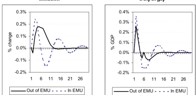
Figure 1 shows the impact of a 1 per cent temporary asymmetric demand shock30 _{on the} UK when it is inside and outside EMU. As might be expected, the economy displays a distinctly more cyclical and volatile response to asymmetric demand shocks inside EMU.

Figure 1: The effect of an asymmetric demand shock on the UK inside and outside EMU (percentage deviation from base)

Inflation Output gap

-0.2% -0.1% 0.0% 0.1% 0.2% 0.3% 1 6 11 16 21 26 % c han ge

Out of EMU In EMU

-0.2% -0.1% 0.0% 0.1% 0.2% 0.3% 0.4% 1 6 11 16 21 26 % G D P

Out of EMU In EMU

30 _{The shock returns to zero with an autoregressive parameter of 0.5. Both inside and outside EMU the} effect of the automatic stabilisers are allowed for and the simple debt solvency rule discussed in section 3.2.2 is also applied from period 6.

In the model, there are three main factors which determine the response of the economy to economic shocks: the role of real interest rates, the role of the real exchange rate and the split between movements in the nominal exchange rate and relative prices.

Outside EMU, a well-designed monetary policy will deliver counter-cyclical real interest rate movements. But inside EMU, the nominal interest rate is fixed by the ECB, which responds to Euro area inflation pressures, rather than UK inflation. Hence movements in the real interest rate could be driven by UK inflation movements. This means that if a positive demand shock led to an increase in UK inflation which was not matched by the rest of the euro area, the real interest rate would actually fall.

The other main channel of adjustment is through movements in the real exchange rate. In the short run, an inflationary shock to the UK alone would cause competitiveness to deteriorate relative to the Euro area, which then limits demand. Within EMU, the real exchange rate adjustment needed to stabilise the economy is greater than would be the case outside EMU because real interest rates are a destabilising influence.

Further, outside EMU, the required relative price adjustment is shared between price changes in the UK and the Euro area and changes in the nominal exchange rate. Inside EMU, the nominal exchange rate between the UK and the Euro area is fixed. This means that the UK price level is anchored by the euro area price level. Hence if the UK price level rises due to an asymmetric demand shock, inflation must be returned below base levels in order to restore the relative price level between the UK and the euro area (as would be the case under a regime of domestic UK price level targeting). This can only be achieved by a fall in the output gap below base levels. Then inflation needs to rise back towards the base level again, requiring a period when output is above base again. This explains the inherently cyclical response to the asymmetric shock for the UK in EMU. Westaway (2003) simulates the model under a variety of shocks to explore how much greater volatility might be expected to be within EMU. For asymmetric shocks, the long-run level of output and inflation variability always increases within EMU. However symmetric shocks are likely to have more modest effects, implying a small trade-off between output and inflation volatility, with inflation volatility rising but output volatility falling. As might be expected, exchange rate shocks (shocks to the sterling-euro risk premium) have a much smaller effect within EMU. However this last result could be reversed if exchange rate shocks (between sterling-euro and sterling-US) are negatively correlated.

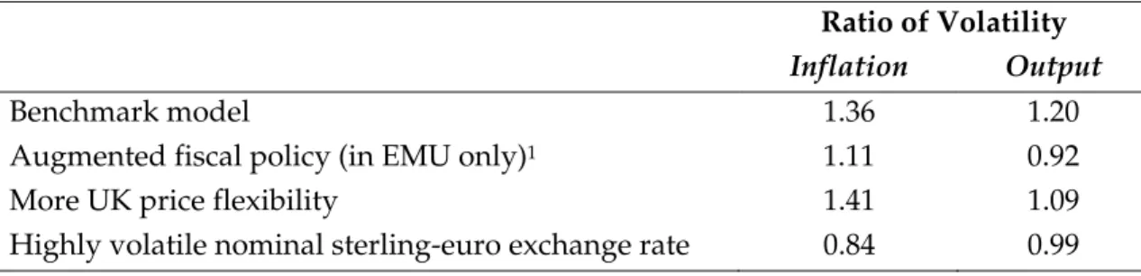
Using an SVAR model to calibrate the set of shocks used for stochastic simulation, Westaway (2003) finds that the benchmark model predicts a rise in both inflation and output volatility inside EMU, by 36 and 20 per cent respectively. However this could be modified or even reversed depending on assumptions about exchange rate shocks in particular. The results suggest allowing a discretionary fiscal policy response may reduce inflation and output volatility markedly. 31

Table 2: Long-Run Volatility Comparison EMU versus non-EMU

Ratio of Volatility

Inflation Output

Benchmark model 1.36 1.20

Augmented fiscal policy (in EMU only)1 _{1.11 0.92}

More UK price flexibility 1.41 1.09

Highly volatile nominal sterling-euro exchange rate 0.84 0.99

Source: HM Treasury (2003b), page 94.

1 _{Assumes a ‘Taylor rule’ for discretionary fiscal policy inside EMU only as described in section 3.2.2 below.}

3.2.2 Modelling the fiscal stabilisation rule

The default version of the model specifies that fiscal policy responds via the automatic stabilisers, ie:

f = -0.5*y

where f is the fiscal impulse and y is the level of output. The coefficient 0.5 is chosen to be consistent with the estimates in Van den Noord (2000).

The following simple stabilisation rules are also considered:

f = -0.5*y + -0.5*(ygap) (Output based rule)

31 _{Kirsanova, Satchi and Vines (2004) use a micro-founded model to look at the role of fiscal stabilisation} policy in a monetary union. They find that active fiscal policy can lead to significant reductions in fluctuations in inflation and output and is most useful in dealing with asymmetric shocks (indeed it can even be slightly detrimental if used to respond to symmetric shocks). They assess the gains using a micro-founded social welfare function and find that fiscal stabilisation leads to significant gains in welfare. These welfare gains increase with the degree of inflation persistence and the longer the output lags are in the Phillips Curve. In addition, while the gains for a simple feedback rule, as modelled here, are less than with a more sophisticated active fiscal policy, they are still sizeable relative to the case with a constant deficit or constant government spending.

f = -0.5*y + -0.5*(ygap) + -0.5*(π – π*) ("Taylor" rule)

where π is the inflation rate, π* _{is the target inflation rate and ygap is the output gap (the}

percentage difference between actual output and potential output). Westaway showed that fiscal rules that actively responded to cyclical deviations in inflation and output helped to reduce the size of those deviations in response to asymmetric demand shocks. Both inside and outside EMU, the automatic stabilisers are allowed to operate. We apply discretionary fiscal policy only to the case within EMU, to show how much discretionary fiscal policy can or cannot compensate for the loss of independent monetary policy. In addition, a debt variable can be added to the model allowing a simple feedback rule for debt32_:

debt = f + (1+r)*debt(-1)

where r is the real interest rate and:

f = [stabilisation rule] + a*f(-1) + b*debt(-1)

The coefficients on the debt rule were chosen arbitrarily.33 _{It is assumed that the initial} level of debt is zero in the model. The debt rule acts to return debt to the base level and helps to prevent explosive behaviour in debt when, as in the case of a permanent supply shock, there are permanent effects on the automatic stabilisers via the effect on output.34

32 _{The UK’s fiscal rules include a net debt-GDP target. As noted it is intended this would be maintained} inside EMU. A discussion of the role of the debt target in the UK’s fiscal rules, and its justification can be found in Woods (2003).

33 _{For most of the simulations the coefficient on the fiscal deficit/surplus was -0.3, while the coefficient on} last period's debt, b, was set at –0.1. The debt solvency rule was applied from period 6 onwards.

34 _{Leith and Wren-Lewis (2004) note that fiscal policy is potentially a more complex instrument for} stabilisation policy than monetary policy in that it can influence the natural level of output, and the use of fiscal policy for stabilisation purposes directly affects the government's inter-temporal budget constraint (IBC). This does not mean that the introduction of fiscal policy as a policy instrument necessarily changes the objective function. However the use of fiscal policy has some potentially interesting implications for how the policy objective function translates into policy targets. For example, in Benigno and Woodford (2003) the Phillips Curve includes a "tax gap" which represents the difference between the actual tax rate and the tax change needed to offset any cost-push shock in order to allow the simultaneous stabilisation of inflation and the output gap. However, the required tax change may be incompatible with meeting the IBC. The results that emerge from Benigno and Woodford (2003) cover a number of different cases, including that of nominal non-state contingent debt and flexible prices (so that the IBC could in theory be met through surprise inflation), real debt with/without sticky prices, and nominal non-state contingent debt and sticky prices (so that inflation alone cannot be used to meet the IBC). The last case has the interesting result that it is no longer optimal to completely offset the fiscal effects of the shock on the government's debt

Two different shocks are illustrated below – a temporary demand shock and a permanent supply shock.

Aggregate demand shock

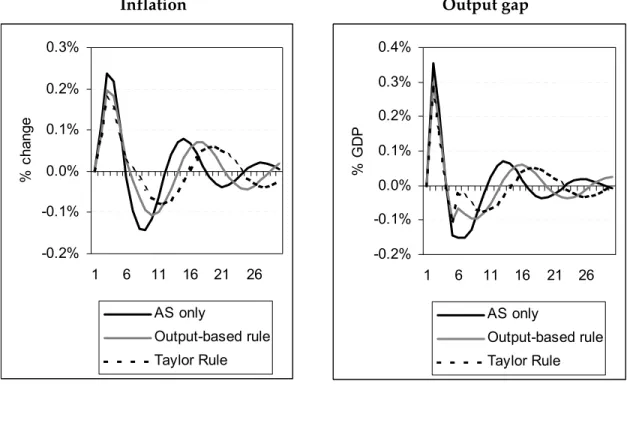
Figure 2 shows the impact on the output gap and inflation of the same 1 per cent temporary asymmetric demand shock as in Figure 1, and the size of the fiscal impulse for different fiscal rules. The baseline setting assumes that only the automatic stabilisers operate (labelled AS only).

Figure 2: Positive Asymmetric Demand Shock for the UK inside EMU with different fiscal policy settings

Inflation Output gap

-0.2% -0.1% 0.0% 0.1% 0.2% 0.3% 1 6 11 16 21 26 % c han ge AS only Output-based rule Taylor Rule -0.2% -0.1% 0.0% 0.1% 0.2% 0.3% 0.4% 1 6 11 16 21 26 % G D P AS only Output-based rule Taylor Rule

stock; instead some drift in the level of debt is optimal, because there are costs to changing distortionary taxation. This does not, however, take account of the possible positive reputational effects of a debt target.

Fiscal impulse Debt level -0.4% -0.2% 0.0% 0.2% 0.4% 0.6% 1 6 11 16 21 26 % G D P AS only Output-based rule Taylor Rule -0.8% -0.6% -0.4% -0.2% 0.0% 0.2% 0.4% 0.6% 0.8% 1 6 11 16 21 26 % G D P AS only Output-based rule Taylor Rule

Using discretionary fiscal policy in EMU helps to reduce the volatility of both inflation and output – as illustrated in Table 2. Because inflation is increasing along with output, an inflation and output gap-based rule stabilises output more than one solely based on the output gap. This is because in this model, increasing the size of the fiscal impulse dampens the shock contemporaneously as there are no lags in fiscal policy's effect. Effectively the shock could be eliminated with an appropriately sized fiscal impulse responding to either inflation or output or a combination of the two.

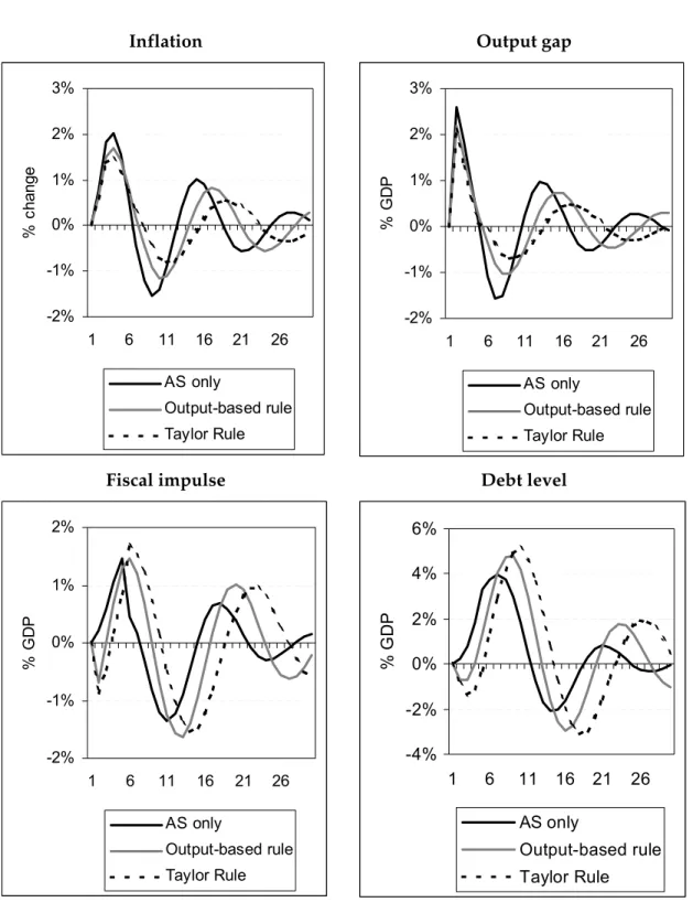
Permanent aggregate supply shock

In this case a permanent 3 per cent fall in supply is simulated. Because prices are slow to adjust, output does not fall by 3 per cent immediately and so there is a positive output gap. With output less than potential, prices rise initially even though output is falling – Figure 3. As with an aggregate demand shock, output and inflation display an oscillatory pattern, reflecting the nature of the adjustment mechanism within EMU.

Figure 3: Permanent aggregate supply shock

Inflation Output gap

-2% -1% 0% 1% 2% 3% 1 6 11 16 21 26 % c han ge AS only Output-based rule Taylor Rule -2% -1% 0% 1% 2% 3% 1 6 11 16 21 26 % G D P AS only Output-based rule Taylor Rule

Fiscal impulse Debt level

-2% -1% 0% 1% 2% 1 6 11 16 21 26 % G D P AS only Output-based rule Taylor Rule -4% -2% 0% 2% 4% 6% 1 6 11 16 21 26 % G D P AS only Output-based rule Taylor Rule

Since the automatic stabilisers are based on the level of output, rather than the output gap, they tend to work in the wrong direction. Lower output therefore leads to a positive fiscal impulse. However an output gap-based fiscal rule would work in the opposite direction, lowering output through tighter fiscal policy to close the output gap.

In addition, because inflation initially rises (because of the positive output gap), an inflation and output-gap based rule would also work to stabilise output.35 _Obviously, the success of this strategy depends critically on the government's ability to identify the supply shock and estimate the output gap correctly. This would not be straightforward. As the level of output is permanently lower, this also means that the automatic stabilisers would have a permanently negative effect on fiscal policy (for example, it might mean that the tax take was permanently lower). Unless fiscal policy were adjusted to take account of this, the level of debt would continue to rise forever, hence the need for a debt term in the fiscal rule in this case.

Changing the feedback on the debt rule

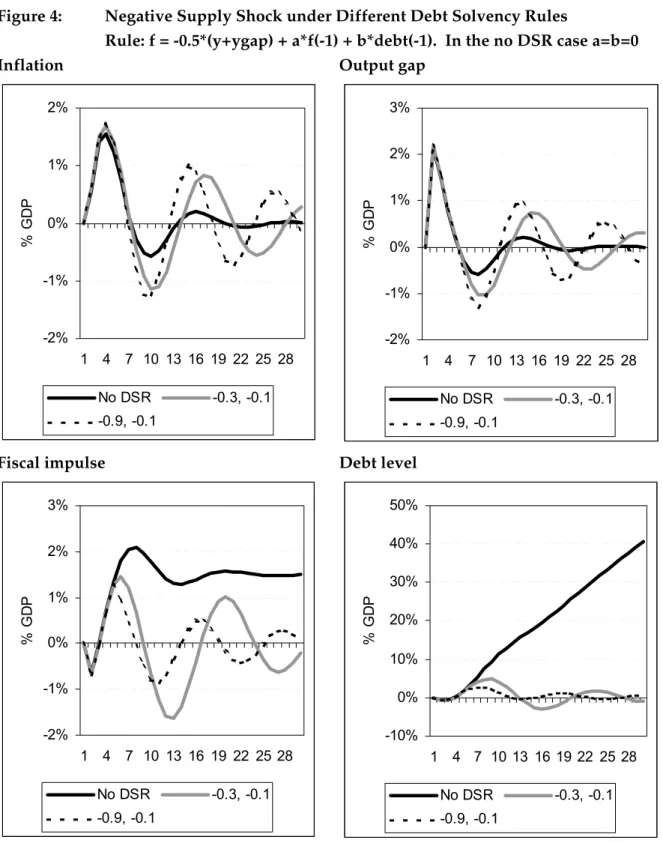
Figure 4 illustrates the effect of changing the strength of the feedback on debt in the fiscal rule, while Table 3 summarises the overall impact on the volatility of inflation, output and the fiscal variables. They illustrate two key points:

• Without a debt rule and a permanent supply shock, the debt-GDP ratio would not be stabilised. This would be inconsistent with the UK’s set of fiscal rules; • A debt rule will affect the scope for fiscal stabilisation. The stronger the feedback

rule, the more volatile output and inflation are likely to be.

35 _{This is not the case outside EMU; inflation initially rises due to the exchange rate response, so that an} inflation-based stabilisation rule would tend to work in the wrong direction to stabilise output (see Westaway (2003) pages 40-42.

Figure 4: Negative Supply Shock under Different Debt Solvency Rules

Rule: f = -0.5*(y+ygap) + a*f(-1) + b*debt(-1). In the no DSR case a=b=0

Inflation Output gap

-2% -1% 0% 1% 2% 1 4 7 10 13 16 19 22 25 28 % G D P No DSR -0.3, -0.1 -0.9, -0.1 -2% -1% 0% 1% 2% 3% 1 4 7 10 13 16 19 22 25 28 % G D P No DSR -0.3, -0.1 -0.9, -0.1

Fiscal impulse Debt level

-2% -1% 0% 1% 2% 3% 1 4 7 10 13 16 19 22 25 28 % G D P No DSR -0.3, -0.1 -0.9, -0.1 -10% 0% 10% 20% 30% 40% 50% 1 4 7 10 13 16 19 22 25 28 % G D P No DSR -0.3, -0.1 -0.9, -0.1

Table 3: Absolute percentage deviation from base over 30 periods (per cent)1

Debt solvency rule No debt solvency rule f = -0.3*f(-1) - 0.1*debt(-1) f = -0.9*f(-1) - 0.1*debt(-1) Inflation 9.0 17.8 18.8 Output 8.0 15.7 17.9 Fiscal impulse 41.9 21.4 11.5 Debt 570.1 51.3 23.5

1_{Note all the fiscal rule also include the terms from the ‘output gap rule’ on page 19.} 3.2.3 The role of a trigger value in the fiscal stabilisation rule

HM Treasury (2003a) proposed that the fiscal stabilisation rule should operate with a trigger value in the fiscal stabilisation rule, whereby discretionary fiscal policy would be only applied when the output gap was expected to exceed +/- 1.5 per cent.36 _{In the sort} of simple model described above, a trigger rule would clearly be less effective than a continuous one.

However, there are a number of possible justifications for a trigger approach. If fixed costs are allowed for, then this can lead to non-linearities in decision-making; for example, price adjustment.37 _{Similarly, allowing for fixed costs in changing the fiscal} instrument should lead to a non-linear fiscal rule. For example, if the preferred fiscal instrument were VAT, then retailers would incur fixed costs such as changing price labels, re-programming cash registers, and so on. Another reason why a trigger rule may be appropriate is the presence of uncertainty. This is likely to be particularly pertinent in relation to uncertainty over the size of the output gap and/or the appropriate path of the real exchange rate and there may be a range over which it would be better to take no action, rather than risk inadvertently pro-cyclical fiscal outcomes. In the UK case, the idea of a trigger rule was also that it would be used to promote an extra layer of transparency and to signal that the stabilisation rule was not intended for ‘fiscal fine tuning’ but rather only to counter-act more sustained cyclical fluctuations.

Choosing the trigger point

In HM Treasury (2003a) the proposed fiscal stabilisation rule does not strictly imply a commitment to keep the output gap within a particular range, rather it implies a

36 _{The Swedish Committee on Stabilisation Policy in EMU (Government of Sweden, 2002) also proposed} that discretionary fiscal action should be reserved for major shocks roughly equivalent to an absolute output gap of 2 per cent.

commitment to say what action would be taken when its forecast appears to breach a certain level, and to give a full explanation of events at this time. But the trigger point would be an indicator of the frequency with which the government intends to act and the degree of variation in the output gap (or inflation) that it deems acceptable without taking any offsetting action.

A high value for the trigger point would mean that fiscal policy would be less active and therefore output could be more volatile than may be desirable from a stabilisation perspective. A low value would mean that discretionary fiscal policy would be used relatively frequently. As discussed, overly frequent use of fiscal policy could be costly, for example in terms of the compliance costs on businesses.

One way of thinking about the appropriate target range is to consider the implications of different levels of volatility for the variable in question. Table 4 shows the probability of exceeding the target range for inflation for different levels of volatility and different target ranges. For example, if UK inflation were to follow the experience since 1997 when outturns have been very stable, then there would only be a very small chance of exceeding a target range which was plus or minus one per cent of the mean target rate (i.e., for a mean target rate of 2 per cent, there would be less than 1 per cent probability of exceeding a target range of 1 to 3 per cent).

However, as discussed above in EMU, the volatility of inflation would be expected to rise; for example, Westaway's (2003) estimates suggest that inflation could be 36 per cent more volatile within EMU (as in Table 2). The second line of the table looks at the chance of exceeding the trigger range adjusting the standard deviation of inflation upwards by 36 per cent. This still suggests that there would still be a low probability of moving much outside a range of +/-1 per cent. Conversely, if inflation were to follow the UK’s experience of the past 25 years then inflation volatility would be considerably higher and inflation would be outside a range of +/-1 per cent most of the time.

Table 4: Probability of exceeding the target value for the CPI inflation rate (as a percentage)

Trigger value +/- x percentage points

0.5 1 1.5 2

Since 1997 (SD = 0.4) 16 1 0 0

Since 1997, adjusted for the estimated increase

in volatility in EMU (SD = 0.5) 30 4 0 0

Since 1979 (SD = 4.0) 90 80 71 62

SD – standard deviation

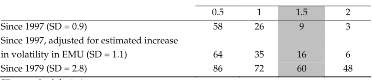
Using the same reference periods, Table 5 derives similar probabilities for the output gap. Hence using the period since 1997 as the reference, the standard deviation of the output gap is 0.9. This suggests that there would be just under a 10 per cent chance of breaching a trigger range of +/-1.5 percentage points (where the expected mean output gap was zero). However, Westaway's estimates suggest that the output gap could be 20 per cent more volatile within EMU (as in Table 2). This would then imply a 16 per cent chance of going outside the 1.5 per cent "band" for the output gap. Again taking the period since 1979 the standard deviation is much higher, implying a 60 per cent chance of exceeding the trigger value.

Table 5: Probability of exceeding the target range for the output gap (as a percentage) Trigger range +/- x percentage points

0.5 1 1.5 2

Since 1997 (SD = 0.9) 58 26 9 3

Since 1997, adjusted for estimated increase

in volatility in EMU (SD = 1.1) 64 35 16 6

Since 1979 (SD = 2.8) 86 72 60 48

SD – standard deviation

One point to note is that the comparative "range" for inflation appears to be considerably narrower than that for output, reflecting greater volatility in outturns for the output gap since 1997.38 _{If one took these figures at face value, they would suggest a relatively} "tight" target range for inflation. However, there is a possibility that the Westaway simulations understate how much more volatile inflation outturns might be within EMU; for example, Minford (2001) found that inflation could be as much as 3 times more

38 _{Note that if the period since 1979 is taken as a reference the output gap range is actually slightly} narrower.

volatile within EMU compared with inflation outside of EMU. Westaway (2003) suggests a number of different factors which might influence the volatility of inflation inside EMU versus outside EMU, including the degree of price flexibility, and the nature of the shocks to the exchange rate (for example, what proportion of the shocks are nominal shocks; whether shocks to the £-€ and £-$ exchange rates are correlated). The stochastic simulations are also affected by the period the shocks are drawn from. The arguments above concerning the need for real exchange rate adjustments to occur through differential inflation rates in EMU might also suggest a wider range was tolerated before any action were taken.

3.3 The operation of the fiscal stabilisation rule within the EU15

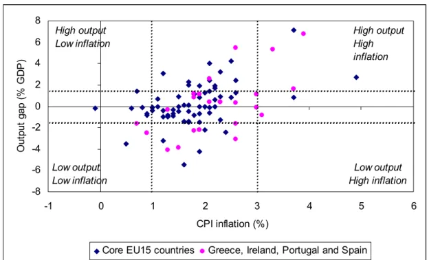
Figure 5 shows how often these sort of stabilisation rules might have been triggered in the EU15 over the recent past. It provides a broad illustration based on data from the European Commission's Spring 2004 forecasts, with each point in the figure representing one of the countries in one year. The figure shows a number of occasions where countries have had output gaps greater than 1½ per cent of GDP in absolute terms, suggesting a case for fiscal tightening. It also shows that were the rule defined in terms of inflation, there would also have been occasions where trigger values of 1 and 3 per cent would have been exceeded. Importantly, for the output gap series, the figures are based on the current EC data and projections. For the historic data these are therefore ex post readings rather than the ex ante readings envisaged in the fiscal stabilisation rule in the HM Treasury (2003a) proposal. 39

39 _{The ex ante readings tend to be closer to the ‘desired’ levels suggesting action would be less likely to} have been triggered than implied in the figures.

Figure 5: Output and inflation in the EU15 countries (1999-2005) -8 -6 -4 -2 0 2 4 6 8 0 1 2 3 4 5 CPI inflation (%) O ut pu t ga p ( % G D P ) 6

Core EU15 countries Greece, Ireland, Portugal and Spain

High output Low inflation High output High inflation Low output Low inflation Low output High inflation

Source: EC Spring 2004 forecasts.

In some countries inflation has been consistently above the EU average. In particular, the figure highlights that the inflation outturns for Greece, Ireland, Spain and Portugal were high relative to their output gap readings. This may reflect the need for some form of real exchange adjustment. For these countries, a higher inflation trigger range may be more appropriate, at least as a temporary measure.

Persistent real exchange rate differentials may reflect Balassa-Samuelson-type effects. This occurs when the productivity differential between the traded and non-traded sectors in a country is larger than in the rest of the euro area. This means that the relative price of non-traded goods will tend to rise more quickly in that country, leading to a real exchange rate appreciation and a sustainable positive inflation differential. This sort of effect can be taken into account by subtracting estimates of the Balassa-Samuelson effect from the above inflation figures – figure 6. This reduces the degree to which the likes of Greece, Ireland, Spain and Portugal might have breached the inflation trigger range on the up side. Due to the Balassa-Samuelson effect, these countries can sustain a higher rate of inflation without suffering from a loss of competitiveness.

Figure 6: Output and inflation in the EU15 countries (1999-2005)

Adjusted for Balassa-Samuelson effects40

-8 -6 -4 -2 0 2 4 6 8 -1 0 1 2 3 4 5 CPI inflation (%) O ut pu t ga p (% G D P ) 6

Core EU15 countries Greece, Ireland, Portugal and Spain

High output Low inflation High output High inflation Low output Low inflation Low output High inflation

Source: EC Spring 2004 forecasts.

3.4 Fiscal stabilisation and the Stability and Growth Pact

The UK Government has consistently argued for a prudent interpretation of the Stability and Growth Pact, grounded in a sound economic rationale, which takes account of the economic cycle and is applied symmetrically throughout the cycle; which distinguishes between high and low debt countries; and which allows for borrowing for public investment within prudent limits. A prudent interpretation would lock in long-term fiscal discipline and sustainability, enhance credibility across the economic cycle, while allowing the automatic stabilisers to operate fully and symmetrically to smooth fluctuations in output, and allow appropriate increases in investment in public services. The HM Treasury (2004) discussion paper argued that in considering the development of the Pact, the issue is not fundamental overhaul or Treaty change, but evolution. And there would need to be extensive discussion before specific proposals could be developed. The paper then set out principles to shape the future discussion and assess future proposals for reform. In particular: the need for clear objectives based on the elements of a prudent interpretation; the importance of pre-commitment to sound

40 _{Estimates of the Balassa-Samuelson effects taken from ECB (2003). Estimates were not available for} Sweden, Denmark and the UK and an adjustment of 0.1 percentage points was applied (i.e. the same as for France and the Netherlands).

institutional arrangements and clear procedural rules, recognising the importance of national fiscal rules that are consistent with the Pact; and the case for independent surveillance and transparency. Using these principles to guide and evaluate future reforms should help in providing credibility, flexibility and legitimacy necessary for an effective macroeconomic framework. In terms of discretionary fiscal action Balls (2004) argued in a recent speech that:

“The challenge is to find institutional arrangements which can both enforce discipline in the above trend phase and in high debt countries and at the same time credibly sanction exceptional fiscal action in low debt countries during a downturn.”

Balls (2004) also noted that a fiscal trigger rule based on an output gap of +/- 1½ per cent would have been triggered in only a few cases where output was below trend (Germany, Portugal and the Netherlands) but many more countries in the early years of EMU would have had to respond when output was above trend - few of which actually tightened fiscal policy:

“… far from sanctioning imprudence, such a Stability and Growth Pact applied symmetrically over the economic cycle would have led to fiscal tightening in a number of higher debt countries or fiscal open letters explaining why fiscal tightening was not, in fact, necessary for the Council to consider. The result should have been more fiscal consolidation in the early years of EMU when economies were largely above trend. And in the below trend phase, while allowing the automatic stabilisers to work, there would not have been a rash of open letters proposing discretionary fiscal loosening.”41

There are signs that the implementation of the Pact is evolving towards a more prudent interpretation. Over the past two years the Council has approved: a greater focus on cyclical adjustment; a recognition the automatic stabilisers should be allowed to operate symmetrically over the cycle; a greater focus on long-run sustainability, including the impact of ageing populations; a greater emphasis on debt reduction in highly indebted countries; and greater attention to the quality of public finances.

4. Discretionary fiscal policy - instruments

HM Treasury (2003a) considered various fiscal instruments that could be used in a discretionary manner for stabilisation purposes. Key criteria for such instruments were to: maximise the impact on activity for a given change in the deficit, minimise lags, and minimise any adverse impacts on wider government objectives such as equity and efficiency. Frequent changes in government expenditure would conflict with the current multi-year spending review structure and could impact on other public policy objectives such as delivering public services.42 _{Hence the focus was on tax instruments, such as:}

Direct taxes: however, varying income taxes or national insurance contributions is likely to generate significant practical problems and may have only a relatively limited stabilisation impact. They are thus unlikely to be suitable instruments for stabilisation purposes.

Consumer credit tax: such a tax could impact on household spending decisions through the effect on borrowing to finance consumption. However, HM Treasury (2003a) that such a tax would not be feasible, all the more so in an integrated EU financial market;

Investment instruments: temporary tax credits could, for example, be used to stimulate investment in a recession. However, the effectiveness of such a measure might be limited, and frequent use of temporary tax incentives could increase uncertainty, damaging long-run investment in the economy;

Housing taxes: fiscal instruments impacting on the housing market could help reduce volatility in this sector of the economy, through automatic stabiliser properties, as well as potentially providing an additional discretionary stabilisation tool. HM Treasury (2003a) considered stamp duty and the wide variety of property taxes levied in other countries;

Expenditure taxes: temporary changes to a combination of expenditure taxes, for example through the regulator power, could prove useful instruments with limited undesirable impacts on incentives, the supply side or the overall equity of the tax system.

This section briefly presents some new work commissioned by HM Treasury from National Institute of Economic and Social Research (NIESR) to examine the effectiveness