OpenFOAM
The Open Source CFD Toolbox
User Guide
Version 3.0.1
13th December 2015
Copyright c° 2011-2015 OpenFOAM Foundation Ltd. Author: Christopher J. Greenshields, CFD Direct Ltd. This work is licensed under a
Creative Commons Attribution-NonCommercial-NoDerivs 3.0 Unported License.
Typeset in LATEX.
License
THE WORK (AS DEFINED BELOW) IS PROVIDED UNDER THE TERMS OF THIS CRE-ATIVE COMMONS PUBLIC LICENSE (“CCPL” OR “LICENSE”). THE WORK IS PRO-TECTED BY COPYRIGHT AND/OR OTHER APPLICABLE LAW. ANY USE OF THE WORK OTHER THAN AS AUTHORIZED UNDER THIS LICENSE OR COPYRIGHT LAW IS PRO-HIBITED.
BY EXERCISING ANY RIGHTS TO THE WORK PROVIDED HERE, YOU ACCEPT AND AGREE TO BE BOUND BY THE TERMS OF THIS LICENSE. TO THE EXTENT THIS LI-CENSE MAY BE CONSIDERED TO BE A CONTRACT, THE LICENSOR GRANTS YOU THE RIGHTS CONTAINED HERE IN CONSIDERATION OF YOUR ACCEPTANCE OF SUCH TERMS AND CONDITIONS.
1. Definitions
a. “Adaptation” means a work based upon the Work, or upon the Work and other pre-existing works, such as a translation, adaptation, derivative work, arrangement of music or other alterations of a literary or artistic work, or phonogram or performance and includes cine-matographic adaptations or any other form in which the Work may be recast, transformed, or adapted including in any form recognizably derived from the original, except that a work that constitutes a Collection will not be considered an Adaptation for the purpose of this License. For the avoidance of doubt, where the Work is a musical work, performance or phonogram, the synchronization of the Work in timed-relation with a moving image (“synching”) will be considered an Adaptation for the purpose of this License.
b. “Collection” means a collection of literary or artistic works, such as encyclopedias and an-thologies, or performances, phonograms or broadcasts, or other works or subject matter other than works listed in Section 1(f) below, which, by reason of the selection and arrange-ment of their contents, constitute intellectual creations, in which the Work is included in its entirety in unmodified form along with one or more other contributions, each constituting separate and independent works in themselves, which together are assembled into a collec-tive whole. A work that constitutes a Collection will not be considered an Adaptation (as defined above) for the purposes of this License.
c. “Distribute” means to make available to the public the original and copies of the Work through sale or other transfer of ownership.
d. “Licensor” means the individual, individuals, entity or entities that offer(s) the Work under the terms of this License.
e. “Original Author” means, in the case of a literary or artistic work, the individual, individuals, entity or entities who created the Work or if no individual or entity can be identified, the
publisher; and in addition (i) in the case of a performance the actors, singers, musicians, dancers, and other persons who act, sing, deliver, declaim, play in, interpret or otherwise perform literary or artistic works or expressions of folklore; (ii) in the case of a phonogram the producer being the person or legal entity who first fixes the sounds of a performance or other sounds; and, (iii) in the case of broadcasts, the organization that transmits the broadcast.
f. “Work” means the literary and/or artistic work offered under the terms of this License including without limitation any production in the literary, scientific and artistic domain, whatever may be the mode or form of its expression including digital form, such as a book, pamphlet and other writing; a lecture, address, sermon or other work of the same nature; a dramatic or dramatico-musical work; a choreographic work or entertainment in dumb show; a musical composition with or without words; a cinematographic work to which are assimilated works expressed by a process analogous to cinematography; a work of drawing, painting, architecture, sculpture, engraving or lithography; a photographic work to which are assimilated works expressed by a process analogous to photography; a work of applied art; an illustration, map, plan, sketch or three-dimensional work relative to geography, topography, architecture or science; a performance; a broadcast; a phonogram; a compilation of data to the extent it is protected as a copyrightable work; or a work performed by a variety or circus performer to the extent it is not otherwise considered a literary or artistic work.
g. “You” means an individual or entity exercising rights under this License who has not pre-viously violated the terms of this License with respect to the Work, or who has received express permission from the Licensor to exercise rights under this License despite a previous violation.
h. “Publicly Perform” means to perform public recitations of the Work and to communicate to the public those public recitations, by any means or process, including by wire or wireless means or public digital performances; to make available to the public Works in such a way that members of the public may access these Works from a place and at a place individu-ally chosen by them; to perform the Work to the public by any means or process and the communication to the public of the performances of the Work, including by public digital performance; to broadcast and rebroadcast the Work by any means including signs, sounds or images.
i. “Reproduce” means to make copies of the Work by any means including without limitation by sound or visual recordings and the right of fixation and reproducing fixations of the Work, including storage of a protected performance or phonogram in digital form or other electronic medium.
2. Fair Dealing Rights.
Nothing in this License is intended to reduce, limit, or restrict any uses free from copyright or rights arising from limitations or exceptions that are provided for in connection with the copyright protection under copyright law or other applicable laws.
3. License Grant.
Subject to the terms and conditions of this License, Licensor hereby grants You a worldwide, royalty-free, non-exclusive, perpetual (for the duration of the applicable copyright) license to ex-ercise the rights in the Work as stated below:
a. to Reproduce the Work, to incorporate the Work into one or more Collections, and to Reproduce the Work as incorporated in the Collections;
b. and, to Distribute and Publicly Perform the Work including as incorporated in Collections. The above rights may be exercised in all media and formats whether now known or hereafter devised. The above rights include the right to make such modifications as are technically necessary to exercise the rights in other media and formats, but otherwise you have no rights to make Adaptations. Subject to 8(f), all rights not expressly granted by Licensor are hereby reserved, including but not limited to the rights set forth in Section 4(d).
4. Restrictions.
The license granted in Section 3 above is expressly made subject to and limited by the following restrictions:
a. You may Distribute or Publicly Perform the Work only under the terms of this License. You must include a copy of, or the Uniform Resource Identifier (URI) for, this License with every copy of the Work You Distribute or Publicly Perform. You may not offer or impose any terms on the Work that restrict the terms of this License or the ability of the recipient of the Work to exercise the rights granted to that recipient under the terms of the License. You may not sublicense the Work. You must keep intact all notices that refer to this License and to the disclaimer of warranties with every copy of the Work You Distribute or Publicly Perform. When You Distribute or Publicly Perform the Work, You may not impose any effective technological measures on the Work that restrict the ability of a recipient of the Work from You to exercise the rights granted to that recipient under the terms of the License. This Section 4(a) applies to the Work as incorporated in a Collection, but this does not require the Collection apart from the Work itself to be made subject to the terms of this License. If You create a Collection, upon notice from any Licensor You must, to the extent practicable, remove from the Collection any credit as required by Section 4(c), as requested.
b. You may not exercise any of the rights granted to You in Section 3 above in any manner that is primarily intended for or directed toward commercial advantage or private monetary compensation. The exchange of the Work for other copyrighted works by means of digital file-sharing or otherwise shall not be considered to be intended for or directed toward commercial advantage or private monetary compensation, provided there is no payment of any monetary compensation in connection with the exchange of copyrighted works.
c. If You Distribute, or Publicly Perform the Work or Collections, You must, unless a request has been made pursuant to Section 4(a), keep intact all copyright notices for the Work and provide, reasonable to the medium or means You are utilizing: (i) the name of the Original Author (or pseudonym, if applicable) if supplied, and/or if the Original Author and/or Licensor designate another party or parties (e.g., a sponsor institute, publishing entity, journal) for attribution (“Attribution Parties”) in Licensor’s copyright notice, terms of service or by other reasonable means, the name of such party or parties; (ii) the title of the Work if supplied; (iii) to the extent reasonably practicable, the URI, if any, that Licensor specifies to be associated with the Work, unless such URI does not refer to the copyright notice or licensing information for the Work. The credit required by this Section 4(c) may be implemented in any reasonable manner; provided, however, that in the case of a Collection, at a minimum such credit will appear, if a credit for all contributing authors of Collection appears, then as part of these credits and in a manner at least as prominent as the credits for the other contributing authors. For the avoidance of doubt, You may only use the credit required by this Section for the purpose of attribution in the manner set out above and, by exercising Your rights under this License, You may not implicitly or explicitly assert or imply any connection with, sponsorship or endorsement by the Original Author, Licensor and/or
Attribution Parties, as appropriate, of You or Your use of the Work, without the separate, express prior written permission of the Original Author, Licensor and/or Attribution Parties. d. For the avoidance of doubt:
i. Non-waivable Compulsory License Schemes. In those jurisdictions in which the right to collect royalties through any statutory or compulsory licensing scheme cannot be waived, the Licensor reserves the exclusive right to collect such royalties for any exercise by You of the rights granted under this License;
ii. Waivable Compulsory License Schemes. In those jurisdictions in which the right to collect royalties through any statutory or compulsory licensing scheme can be waived, the Licensor reserves the exclusive right to collect such royalties for any exercise by You of the rights granted under this License if Your exercise of such rights is for a purpose or use which is otherwise than noncommercial as permitted under Section 4(b) and otherwise waives the right to collect royalties through any statutory or compulsory licensing scheme; and,
iii. Voluntary License Schemes. The Licensor reserves the right to collect royalties, whether individually or, in the event that the Licensor is a member of a collecting society that administers voluntary licensing schemes, via that society, from any exercise by You of the rights granted under this License that is for a purpose or use which is otherwise than noncommercial as permitted under Section 4(b).
e. Except as otherwise agreed in writing by the Licensor or as may be otherwise permitted by applicable law, if You Reproduce, Distribute or Publicly Perform the Work either by itself or as part of any Collections, You must not distort, mutilate, modify or take other derogatory action in relation to the Work which would be prejudicial to the Original Author’s honor or reputation.
5. Representations, Warranties and Disclaimer
UNLESS OTHERWISE MUTUALLY AGREED BY THE PARTIES IN WRITING, LICENSOR OFFERS THE WORK AS-IS AND MAKES NO REPRESENTATIONS OR WARRANTIES OF ANY KIND CONCERNING THE WORK, EXPRESS, IMPLIED, STATUTORY OR OTHER-WISE, INCLUDING, WITHOUT LIMITATION, WARRANTIES OF TITLE, MERCHANTIBIL-ITY, FITNESS FOR A PARTICULAR PURPOSE, NONINFRINGEMENT, OR THE ABSENCE OF LATENT OR OTHER DEFECTS, ACCURACY, OR THE PRESENCE OF ABSENCE OF ERRORS, WHETHER OR NOT DISCOVERABLE. SOME JURISDICTIONS DO NOT ALLOW THE EXCLUSION OF IMPLIED WARRANTIES, SO SUCH EXCLUSION MAY NOT APPLY TO YOU.
6. Limitation on Liability.
EXCEPT TO THE EXTENT REQUIRED BY APPLICABLE LAW, IN NO EVENT WILL LI-CENSOR BE LIABLE TO YOU ON ANY LEGAL THEORY FOR ANY SPECIAL, INCIDEN-TAL, CONSEQUENTIAL, PUNITIVE OR EXEMPLARY DAMAGES ARISING OUT OF THIS LICENSE OR THE USE OF THE WORK, EVEN IF LICENSOR HAS BEEN ADVISED OF THE POSSIBILITY OF SUCH DAMAGES.
7. Termination
a. This License and the rights granted hereunder will terminate automatically upon any breach by You of the terms of this License. Individuals or entities who have received Collections
from You under this License, however, will not have their licenses terminated provided such individuals or entities remain in full compliance with those licenses. Sections 1, 2, 5, 6, 7, and 8 will survive any termination of this License.
b. Subject to the above terms and conditions, the license granted here is perpetual (for the duration of the applicable copyright in the Work). Notwithstanding the above, Licensor reserves the right to release the Work under different license terms or to stop distributing the Work at any time; provided, however that any such election will not serve to withdraw this License (or any other license that has been, or is required to be, granted under the terms of this License), and this License will continue in full force and effect unless terminated as stated above.
8. Miscellaneous
a. Each time You Distribute or Publicly Perform the Work or a Collection, the Licensor offers to the recipient a license to the Work on the same terms and conditions as the license granted to You under this License.
b. If any provision of this License is invalid or unenforceable under applicable law, it shall not affect the validity or enforceability of the remainder of the terms of this License, and without further action by the parties to this agreement, such provision shall be reformed to the minimum extent necessary to make such provision valid and enforceable.
c. No term or provision of this License shall be deemed waived and no breach consented to unless such waiver or consent shall be in writing and signed by the party to be charged with such waiver or consent.
d. This License constitutes the entire agreement between the parties with respect to the Work licensed here. There are no understandings, agreements or representations with respect to the Work not specified here. Licensor shall not be bound by any additional provisions that may appear in any communication from You.
e. This License may not be modified without the mutual written agreement of the Licensor and You. The rights granted under, and the subject matter referenced, in this License were drafted utilizing the terminology of the Berne Convention for the Protection of Literary and Artistic Works (as amended on September 28, 1979), the Rome Convention of 1961, the WIPO Copyright Treaty of 1996, the WIPO Performances and Phonograms Treaty of 1996 and the Universal Copyright Convention (as revised on July 24, 1971). These rights and subject matter take effect in the relevant jurisdiction in which the License terms are sought to be enforced according to the corresponding provisions of the implementation of those treaty provisions in the applicable national law. If the standard suite of rights granted under applicable copyright law includes additional rights not granted under this License, such additional rights are deemed to be included in the License; this License is not intended to restrict the license of any rights under applicable law.
Trademarks
ANSYS is a registered trademark of ANSYS Inc. CFX is a registered trademark of Ansys Inc.
CHEMKIN is a registered trademark of Reaction Design Corporation
EnSight is a registered trademark of Computational Engineering International Ltd. Fieldview is a registered trademark of Intelligent Light
Fluent is a registered trademark of Ansys Inc. GAMBIT is a registered trademark of Ansys Inc. Icem-CFD is a registered trademark of Ansys Inc.
I-DEAS is a registered trademark of Structural Dynamics Research Corporation JAVA is a registered trademark of Sun Microsystems Inc.
Linux is a registered trademark of Linus Torvalds OpenFOAM is a registered trademark of ESI Group ParaView is a registered trademark of Kitware
STAR-CD is a registered trademark of Computational Dynamics Ltd. UNIX is a registered trademark of The Open Group
Contents
Copyright Notice U-2
1. Definitions . . . U-2 2. Fair Dealing Rights. . . U-3 3. License Grant. . . U-3 4. Restrictions. . . U-4 5. Representations, Warranties and Disclaimer . . . U-5 6. Limitation on Liability. . . U-5 7. Termination . . . U-5 8. Miscellaneous . . . U-6 Trademarks U-7 Contents U-9 1 Introduction U-15 2 Tutorials U-17
2.1 Lid-driven cavity flow. . . U-17 2.1.1 Pre-processing . . . U-18 2.1.1.1 Mesh generation . . . U-18 2.1.1.2 Boundary and initial conditions . . . U-20 2.1.1.3 Physical properties . . . U-21 2.1.1.4 Control . . . U-22 2.1.1.5 Discretisation and linear-solver settings. . . U-23 2.1.2 Viewing the mesh . . . U-23 2.1.3 Running an application. . . U-24 2.1.4 Post-processing . . . U-25 2.1.4.1 Isosurface and contour plots . . . U-25 2.1.4.2 Vector plots . . . U-27 2.1.4.3 Streamline plots . . . U-29 2.1.5 Increasing the mesh resolution . . . U-29 2.1.5.1 Creating a new case using an existing case . . . U-29 2.1.5.2 Creating the finer mesh . . . U-31 2.1.5.3 Mapping the coarse mesh results onto the fine mesh . . U-31 2.1.5.4 Control adjustments . . . U-32 2.1.5.5 Running the code as a background process . . . U-32 2.1.5.6 Vector plot with the refined mesh . . . U-32 2.1.5.7 Plotting graphs . . . U-33
2.1.6 Introducing mesh grading . . . U-35 2.1.6.1 Creating the graded mesh . . . U-36 2.1.6.2 Changing time and time step . . . U-37 2.1.6.3 Mapping fields . . . U-38 2.1.7 Increasing the Reynolds number . . . U-38 2.1.7.1 Pre-processing . . . U-39 2.1.7.2 Running the code . . . U-39 2.1.8 High Reynolds number flow . . . U-40 2.1.8.1 Pre-processing . . . U-40 2.1.8.2 Running the code . . . U-42 2.1.9 Changing the case geometry . . . U-42 2.1.10 Post-processing the modified geometry . . . U-46 2.2 Stress analysis of a plate with a hole . . . U-46 2.2.1 Mesh generation . . . U-47 2.2.1.1 Boundary and initial conditions . . . U-50 2.2.1.2 Mechanical properties . . . U-51 2.2.1.3 Thermal properties . . . U-51 2.2.1.4 Control . . . U-51 2.2.1.5 Discretisation schemes and linear-solver control . . . . U-52 2.2.2 Running the code . . . U-54 2.2.3 Post-processing . . . U-54 2.2.4 Exercises. . . U-55 2.2.4.1 Increasing mesh resolution . . . U-56 2.2.4.2 Introducing mesh grading . . . U-56 2.2.4.3 Changing the plate size . . . U-56 2.3 Breaking of a dam . . . U-56 2.3.1 Mesh generation . . . U-57 2.3.2 Boundary conditions . . . U-59 2.3.3 Setting initial field . . . U-59 2.3.4 Fluid properties . . . U-60 2.3.5 Turbulence modelling . . . U-61 2.3.6 Time step control . . . U-62 2.3.7 Discretisation schemes . . . U-62 2.3.8 Linear-solver control . . . U-63 2.3.9 Running the code . . . U-64 2.3.10 Post-processing . . . U-64 2.3.11 Running in parallel . . . U-64 2.3.12 Post-processing a case run in parallel . . . U-67
3 Applications and libraries U-69
3.1 The programming language of OpenFOAM . . . U-69 3.1.1 Language in general . . . U-69 3.1.2 Object-orientation and C++ . . . U-70 3.1.3 Equation representation . . . U-70 3.1.4 Solver codes . . . U-71 3.2 Compiling applications and libraries . . . U-71 3.2.1 Header .H files. . . U-71 3.2.2 Compiling with wmake . . . U-73
3.2.2.1 Including headers . . . U-73 3.2.2.2 Linking to libraries . . . U-74 3.2.2.3 Source files to be compiled . . . U-75 3.2.2.4 Running wmake . . . U-75 3.2.2.5 wmake environment variables . . . U-76 3.2.3 Removing dependency lists: wclean and rmdepall . . . U-76 3.2.4 Compilation example: the pisoFoam application . . . U-77 3.2.5 Debug messaging and optimisation switches . . . U-79 3.2.6 Linking new user-defined libraries to existing applications . . . . U-80 3.3 Running applications . . . U-81 3.4 Running applications in parallel . . . U-81 3.4.1 Decomposition of mesh and initial field data . . . U-82 3.4.2 Running a decomposed case . . . U-84 3.4.3 Distributing data across several disks . . . U-84 3.4.4 Post-processing parallel processed cases . . . U-85 3.4.4.1 Reconstructing mesh and data . . . U-85 3.4.4.2 Post-processing decomposed cases . . . U-85 3.5 Standard solvers. . . U-85 3.6 Standard utilities . . . U-90 3.7 Standard libraries . . . U-97
4 OpenFOAM cases U-105
4.1 File structure of OpenFOAM cases . . . U-105 4.2 Basic input/output file format . . . U-106 4.2.1 General syntax rules . . . U-106 4.2.2 Dictionaries . . . U-107 4.2.3 The data file header . . . U-107 4.2.4 Lists . . . U-108 4.2.5 Scalars, vectors and tensors . . . U-109 4.2.6 Dimensional units . . . U-109 4.2.7 Dimensioned types . . . U-110 4.2.8 Fields . . . U-110 4.2.9 Directives and macro substitutions . . . U-111 4.2.10 The #include and #inputMode directives . . . U-112 4.2.11 The #codeStream directive . . . U-112 4.3 Time and data input/output control . . . U-113 4.4 Numerical schemes . . . U-116 4.4.1 Interpolation schemes . . . U-117 4.4.1.1 Schemes for strictly bounded scalar fields . . . U-118 4.4.1.2 Schemes for vector fields . . . U-118 4.4.2 Surface normal gradient schemes . . . U-119 4.4.3 Gradient schemes . . . U-120 4.4.4 Laplacian schemes . . . U-120 4.4.5 Divergence schemes . . . U-121 4.4.6 Time schemes . . . U-122 4.4.7 Flux calculation . . . U-122 4.5 Solution and algorithm control. . . U-123 4.5.1 Linear solver control . . . U-123
4.5.1.1 Solution tolerances . . . U-124 4.5.1.2 Preconditioned conjugate gradient solvers . . . U-125 4.5.1.3 Smooth solvers . . . U-125 4.5.1.4 Geometric-algebraic multi-grid solvers . . . U-125 4.5.2 Solution under-relaxation . . . U-126 4.5.3 PISO and SIMPLE algorithms. . . U-127 4.5.3.1 Pressure referencing . . . U-127 4.5.4 Other parameters . . . U-128
5 Mesh generation and conversion U-129
5.1 Mesh description . . . U-129 5.1.1 Mesh specification and validity constraints . . . U-129 5.1.1.1 Points . . . U-130 5.1.1.2 Faces . . . U-130 5.1.1.3 Cells . . . U-131 5.1.1.4 Boundary . . . U-131 5.1.2 The polyMesh description. . . U-131 5.1.3 The cellShape tools . . . U-132 5.1.4 1- and 2-dimensional and axi-symmetric problems . . . U-133 5.2 Boundaries . . . U-133 5.2.1 Specification of patch types in OpenFOAM. . . U-135 5.2.2 Base types . . . U-136 5.2.3 Primitive types . . . U-138 5.2.4 Derived types . . . U-138 5.3 Mesh generation with theblockMesh utility . . . U-140 5.3.1 Writing a blockMeshDict file . . . U-140 5.3.1.1 The vertices . . . U-141 5.3.1.2 The edges . . . U-142 5.3.1.3 The blocks . . . U-142 5.3.1.4 Multi-grading of a block . . . U-143 5.3.1.5 The boundary . . . U-145 5.3.2 Multiple blocks . . . U-146 5.3.3 Creating blocks with fewer than 8 vertices . . . U-148 5.3.4 RunningblockMesh . . . U-149 5.4 Mesh generation with thesnappyHexMesh utility . . . U-149 5.4.1 The mesh generation process of snappyHexMesh . . . U-149 5.4.2 Creating the background hex mesh . . . U-151 5.4.3 Cell splitting at feature edges and surfaces . . . U-152 5.4.4 Cell removal . . . U-154 5.4.5 Cell splitting in specified regions. . . U-154 5.4.6 Snapping to surfaces . . . U-155 5.4.7 Mesh layers . . . U-155 5.4.8 Mesh quality controls . . . U-158 5.5 Mesh conversion. . . U-158 5.5.1 fluentMeshToFoam . . . U-159 5.5.2 starToFoam . . . U-160 5.5.2.1 General advice on conversion . . . U-160 5.5.2.2 Eliminating extraneous data . . . U-160
5.5.2.3 Removing default boundary conditions . . . U-161 5.5.2.4 Renumbering the model . . . U-162 5.5.2.5 Writing out the mesh data . . . U-163 5.5.2.6 Problems with the .vrt file . . . U-163 5.5.2.7 Converting the mesh to OpenFOAM format . . . U-164 5.5.3 gambitToFoam . . . U-164 5.5.4 ideasToFoam . . . U-164 5.5.5 cfx4ToFoam . . . U-165 5.6 Mapping fields between different geometries . . . U-165 5.6.1 Mapping consistent fields . . . U-165 5.6.2 Mapping inconsistent fields. . . U-166 5.6.3 Mapping parallel cases . . . U-167
6 Post-processing U-169
6.1 paraFoam . . . U-169 6.1.1 Overview of paraFoam . . . U-169 6.1.2 The Parameters panel . . . U-171 6.1.3 The Display panel . . . U-172 6.1.4 The button toolbars . . . U-173 6.1.5 Manipulating the view . . . U-173 6.1.5.1 View settings . . . U-173 6.1.5.2 General settings . . . U-174 6.1.6 Contour plots . . . U-174 6.1.6.1 Introducing a cutting plane . . . U-174 6.1.7 Vector plots . . . U-174 6.1.7.1 Plotting at cell centres . . . U-175 6.1.8 Streamlines . . . U-175 6.1.9 Image output . . . U-175 6.1.10 Animation output . . . U-175 6.2 Function Objects . . . U-176 6.2.1 Using function objects . . . U-177 6.2.2 Packaged function objects . . . U-179 6.3 Post-processing withFluent . . . U-181 6.4 Post-processing withFieldview . . . U-182 6.5 Post-processing withEnSight . . . U-183 6.5.1 Converting data to EnSight format . . . U-183 6.5.2 The ensight74FoamExec reader module . . . U-183 6.5.2.1 Configuration of EnSight for the reader module . . . . U-183 6.5.2.2 Using the reader module . . . U-184 6.6 Sampling data . . . U-184 6.7 Monitoring and managing jobs . . . U-186 6.7.1 The foamJob script for running jobs . . . U-188 6.7.2 The foamLog script for monitoring jobs . . . U-188
7 Models and physical properties U-191
7.1 Thermophysical models . . . U-191 7.1.1 Thermophysical and mixture models . . . U-192 7.1.2 Transport model . . . U-193
7.1.3 Thermodynamic models . . . U-193 7.1.4 Composition of each constituent . . . U-194 7.1.5 Equation of state . . . U-195 7.1.6 Selection of energy variable . . . U-196 7.1.7 Thermophysical property data . . . U-196 7.2 Turbulence models . . . U-197 7.2.1 Model coefficients . . . U-198 7.2.2 Wall functions . . . U-198 7.3 Transport/rheology models. . . U-199 7.3.1 Newtonian model . . . U-199 7.3.2 Bird-Carreau model. . . U-200 7.3.3 Cross Power Law model . . . U-200 7.3.4 Power Law model . . . U-200 7.3.5 Herschel-Bulkley model. . . U-201
Chapter 1
Introduction
This guide accompanies the release of version 3.0.1 of the Open Source Field Operation and Manipulation (OpenFOAM) C++ libraries. It provides a description of the basic operation of OpenFOAM, first through a set of tutorial exercises in chapter 2 and later by a more detailed description of the individual components that make up OpenFOAM.
OpenFOAM is first and foremost a C++ library, used primarily to create executables, known as applications. The applications fall into two categories: solvers, that are each designed to solve a specific problem in continuum mechanics; andutilities, that are designed to perform tasks that involve data manipulation. The OpenFOAM distribution contains numerous solvers and utilities covering a wide range of problems, as described in chapter3. One of the strengths of OpenFOAM is that new solvers and utilities can be created by its users with some pre-requisite knowledge of the underlying method, physics and programming techniques involved.
OpenFOAM is supplied with pre- and post-processing environments. The interface to the pre- and post-processing are themselves OpenFOAM utilities, thereby ensuring consistent data handling across all environments. The overall structure of OpenFOAM is shown in Figure 1.1. The pre-processing and running of OpenFOAM cases is described in chapter 4.
ApplicationsUser Tools
Meshing
Utilities ApplicationsStandard e.g.OthersEnSight Post-processing Solving
Pre-processing
Open Source Field Operation and Manipulation (OpenFOAM) C++ Library
ParaView
Figure 1.1: Overview of OpenFOAM structure.
In chapter 5, we cover both the generation of meshes using the mesh generator supplied with OpenFOAM and conversion of mesh data generated by third-party products. Post-processing is described in chapter 6.
Chapter 2
Tutorials
In this chapter we shall describe in detail the process of setup, simulation and post-processing for some OpenFOAM test cases, with the principal aim of introducing a user to the basic procedures of running OpenFOAM. The$FOAM TUTORIALSdirectory contains many more cases that demonstrate the use of all the solvers and many utilities supplied with Open-FOAM. Before attempting to run the tutorials, the user must first make sure that they have installed OpenFOAM correctly.
The tutorial cases describe the use of the blockMesh pre-processing tool, case setup and running OpenFOAM solvers and post-processing usingparaFoam. Those users with access to third-party post-processing tools supported in OpenFOAM have an option: either they can follow the tutorials using paraFoam; or refer to the description of the use of the third-party product in chapter 6when post-processing is required.
Copies of all tutorials are available from thetutorialsdirectory of the OpenFOAM instal-lation. The tutorials are organised into a set of directories according to the type of flow and then subdirectories according to solver. For example, all theicoFoamcases are stored within a subdirectory incompressible/icoFoam, where incompressible indicates the type of flow. If the user wishes to run a range of example cases, it is recommended that the user copy the tutorials directory into their localrun directory. They can be easily copied by typing:
mkdir -p $FOAM RUN
cp -r $FOAM TUTORIALS $FOAM RUN
2.1
Lid-driven cavity flow
This tutorial will describe how to pre-process, run and post-process a case involving isother-mal, incompressible flow in a two-dimensional square domain. The geometry is shown in Figure 2.1 in which all the boundaries of the square are walls. The top wall moves in the
x-direction at a speed of 1 m/s while the other 3 are stationary. Initially, the flow will be assumed laminar and will be solved on a uniform mesh using the icoFoamsolver for laminar, isothermal, incompressible flow. During the course of the tutorial, the effect of increased mesh resolution and mesh grading towards the walls will be investigated. Finally, the flow Reynolds number will be increased and the pisoFoam solver will be used for turbulent, isothermal, incompressible flow.
x
Ux = 1 m/s
d= 0.1 m
y
Figure 2.1: Geometry of the lid driven cavity.
2.1.1
Pre-processing
Cases are setup in OpenFOAM by editing case files. Users should select an xeditor of choice with which to do this, such as emacs, vi, gedit, kate, nedit, etc. Editing files is possible in OpenFOAM because the I/O uses a dictionary format with keywords that convey sufficient meaning to be understood by even the least experienced users.
A case being simulated involves data for mesh, fields, properties, control parameters, etc. As described in section 4.1, in OpenFOAM this data is stored in a set of files within a case directory rather than in a single case file, as in many other CFD packages. The case directory is given a suitably descriptive name, e.g.the first example case for this tutorial is simply named cavity. In preparation of editing case files and running the first cavity case, the user should change to the case directory
cd $FOAM RUN/tutorials/incompressible/icoFoam/cavity 2.1.1.1 Mesh generation
OpenFOAM always operates in a 3 dimensional Cartesian coordinate system and all geome-tries are generated in 3 dimensions. OpenFOAM solves the case in 3 dimensions by default but can be instructed to solve in 2 dimensions by specifying a ‘special’ empty boundary condition on boundaries normal to the (3rd) dimension for which no solution is required.
The cavity domain consists of a square of side length d = 0.1 m in the x-y plane. A uniform mesh of 20 by 20 cells will be used initially. The block structure is shown in Figure 2.2. The mesh generator supplied with OpenFOAM, blockMesh, generates meshes from a description specified in an input dictionary,blockMeshDict located in thesystem(or constant/polyMesh) directory for a given case. The blockMeshDict entries for this case are as follows:
1 /*---*- C++ -*---*\
2 | ========= | |
3 | \\ / F ield | OpenFOAM: The Open Source CFD Toolbox |
4 | \\ / O peration | Version: 3.0.1 |
5 | \\ / A nd | Web: www.OpenFOAM.org |
3 2 4 5 7 6 0 z x 1 y
Figure 2.2: Block structure of the mesh for the cavity.
7 \*---*/ 8 FoamFile 9 { 10 version 2.0; 11 format ascii; 12 class dictionary; 13 object blockMeshDict; 14 } 15 // * * * * * * * * * * * * * * * * * * * * * * * * * * * * * * * * * * * * * // 16 17 convertToMeters 0.1; 18 19 vertices 20 ( 21 (0 0 0) 22 (1 0 0) 23 (1 1 0) 24 (0 1 0) 25 (0 0 0.1) 26 (1 0 0.1) 27 (1 1 0.1) 28 (0 1 0.1) 29 ); 30 31 blocks 32 ( 33 hex (0 1 2 3 4 5 6 7) (20 20 1) simpleGrading (1 1 1) 34 ); 35 36 edges 37 ( 38 ); 39 40 boundary 41 ( 42 movingWall 43 { 44 type wall; 45 faces 46 ( 47 (3 7 6 2) 48 ); 49 } 50 fixedWalls 51 { 52 type wall; 53 faces 54 ( 55 (0 4 7 3) 56 (2 6 5 1) 57 (1 5 4 0) 58 ); 59 }
60 frontAndBack 61 { 62 type empty; 63 faces 64 ( 65 (0 3 2 1) 66 (4 5 6 7) 67 ); 68 } 69 ); 70 71 mergePatchPairs 72 ( 73 ); 74 75 // ************************************************************************* //
The file first contains header information in the form of a banner (lines 1-7), then file information contained in a FoamFilesub-dictionary, delimited by curly braces ({...}). For the remainder of the manual:
For the sake of clarity and to save space, file headers, including the banner and FoamFilesub-dictionary, will be removed from verbatim quoting of case files
The file first specifies coordinates of the block vertices; it then defines the blocks (here, only 1) from the vertex labels and the number of cells within it; and finally, it defines the boundary patches. The user is encouraged to consult section 5.3 to understand the meaning of the entries in theblockMeshDict file.
The mesh is generated by running blockMesh on this blockMeshDict file. From within the case directory, this is done, simply by typing in the terminal:
blockMesh
The running status of blockMesh is reported in the terminal window. Any mistakes in the blockMeshDict file are picked up by blockMesh and the resulting error message directs the user to the line in the file where the problem occurred. There should be no error messages at this stage.
2.1.1.2 Boundary and initial conditions
Once the mesh generation is complete, the user can look at this initial fields set up for this case. The case is set up to start at time t = 0 s, so the initial field data is stored in a 0 sub-directory of the cavity directory. The 0 sub-directory contains 2 files, p and U, one for each of the pressure (p) and velocity (U) fields whose initial values and boundary conditions must be set. Let us examine file p:
17 dimensions [0 2 -2 0 0 0 0]; 18 19 internalField uniform 0; 20 21 boundaryField 22 { 23 movingWall 24 { 25 type zeroGradient; 26 } 27 28 fixedWalls 29 { 30 type zeroGradient; 31 }
32 33 frontAndBack 34 { 35 type empty; 36 } 37 } 38 39 // ************************************************************************* //
There are 3 principal entries in field data files:
dimensions specifies the dimensions of the field, here kinematic pressure, i.e. m2s−2 (see section 4.2.6 for more information);
internalField the internal field data which can be uniform, described by a single value; or nonuniform, where all the values of the field must be specified (see section 4.2.8 for more information);
boundaryField the boundary field data that includes boundary conditions and data for all the boundary patches (see section 4.2.8 for more information).
For this casecavity, the boundary consists of walls only, split into 2 patches named: (1) fixedWalls for the fixed sides and base of the cavity; (2) movingWall for the moving top of the cavity. As walls, both are given a zeroGradient boundary condition for p, meaning “the normal gradient of pressure is zero”. The frontAndBack patch represents the front and back planes of the 2D case and therefore must be set as empty.
In this case, as in most we encounter, the initial fields are set to be uniform. Here the pressure is kinematic, and as an incompressible case, its absolute value is not relevant, so is set to uniform 0 for convenience.
The user can similarly examine the velocity field in the 0/U file. The dimensions are those expected for velocity, the internal field is initialised as uniform zero, which in the case of velocity must be expressed by 3 vector components, i.e.uniform (0 0 0) (see section 4.2.5 for more information).
The boundary field for velocity requires the same boundary condition for the frontAnd-Backpatch. The other patches are walls: a no-slip condition is assumed on thefixedWalls, hence a fixedValue condition with a value of uniform (0 0 0). The top surface moves at a speed of 1 m/s in the x-direction so requires afixedValuecondition also but withuniform (1 0 0).
2.1.1.3 Physical properties
The physical properties for the case are stored in dictionaries whose names are given the suffix . . . Properties, located in the Dictionaries directory tree. For an icoFoam case, the only property that must be specified is the kinematic viscosity which is stored from the transportProperties dictionary. The user can check that the kinematic viscosity is set correctly by opening thetransportPropertiesdictionary to view/edit its entries. The keyword for kinematic viscosity is nu, the phonetic label for the Greek symbol ν by which it is represented in equations. Initially this case will be run with a Reynolds number of 10, where the Reynolds number is defined as:
Re= d|U|
wheredand|U|are the characteristic length and velocity respectively andνis the kinematic viscosity. Here d= 0.1 m,|U|= 1 m s−1
, so that for Re= 10, ν = 0.01 m2s−1
. The correct file entry for kinematic viscosity is thus specified below:
17 18 nu [0 2 -1 0 0 0 0] 0.01; 19 20 21 // ************************************************************************* // 2.1.1.4 Control
Input data relating to the control of time and reading and writing of the solution data are read in from the controlDictdictionary. The user should view this file; as a case control file, it is located in the systemdirectory.
The start/stop times and the time step for the run must be set. OpenFOAM offers great flexibility with time control which is described in full in section 4.3. In this tutorial we wish to start the run at time t = 0 which means that OpenFOAM needs to read field data from a directory named 0— see section 4.1 for more information of the case file structure. Therefore we set the startFrom keyword to startTime and then specify the startTime keyword to be 0.
For the end time, we wish to reach the steady state solution where the flow is circulating around the cavity. As a general rule, the fluid should pass through the domain 10 times to reach steady state in laminar flow. In this case the flow does not pass through this domain as there is no inlet or outlet, so instead the end time can be set to the time taken for the lid to travel ten times across the cavity, i.e. 1 s; in fact, with hindsight, we discover that 0.5 s is sufficient so we shall adopt this value. To specify this end time, we must specify the stopAt keyword as endTime and then set theendTime keyword to 0.5.
Now we need to set the time step, represented by the keyword deltaT. To achieve temporal accuracy and numerical stability when runningicoFoam, a Courant number of less than 1 is required. The Courant number is defined for one cell as:
Co= δt|U|
δx (2.2)
where δt is the time step, |U| is the magnitude of the velocity through that cell and δx is the cell size in the direction of the velocity. The flow velocity varies across the domain and we must ensure Co < 1 everywhere. We therefore choose δt based on the worst case: the maximum Co corresponding to the combined effect of a large flow velocity and small cell size. Here, the cell size is fixed across the domain so the maximum Co will occur next to the lid where the velocity approaches 1 m s−1
. The cell size is:
δx= d
n =
0.1
20 = 0.005 m (2.3)
Therefore to achieve a Courant number less than or equal to 1 throughout the domain the time step deltaT must be set to less than or equal to:
δt= Co δx |U| =
1×0.005
1 = 0.005 s (2.4)
As the simulation progresses we wish to write results at certain intervals of time that we can later view with a post-processing package. ThewriteControlkeyword presents several
options for setting the time at which the results are written; here we select the timeStep option which specifies that results are written every nth time step where the value n is specified under the writeInterval keyword. Let us decide that we wish to write our results at times 0.1, 0.2,. . . , 0.5 s. With a time step of 0.005 s, we therefore need to output results at every 20th time time step and so we set writeInterval to 20.
OpenFOAM creates a new directory named after the current time, e.g. 0.1 s, on each occasion that it writes a set of data, as discussed in full in section4.1. In theicoFoamsolver, it writes out the results for each field, U and p, into the time directories. For this case, the entries in the controlDict are shown below:
17 18 application icoFoam; 19 20 startFrom startTime; 21 22 startTime 0; 23 24 stopAt endTime; 25 26 endTime 0.5; 27 28 deltaT 0.005; 29 30 writeControl timeStep; 31 32 writeInterval 20; 33 34 purgeWrite 0; 35 36 writeFormat ascii; 37 38 writePrecision 6; 39 40 writeCompression off; 41 42 timeFormat general; 43 44 timePrecision 6; 45 46 runTimeModifiable true; 47 48 49 // ************************************************************************* //
2.1.1.5 Discretisation and linear-solver settings
The user specifies the choice of finite volume discretisation schemes in the fvSchemes dictio-nary in the systemdirectory. The specification of the linear equation solvers and tolerances and other algorithm controls is made in the fvSolution dictionary, similarly in the system directory. The user is free to view these dictionaries but we do not need to discuss all their entries at this stage except for pRefCell and pRefValue in the PISO sub-dictionary of the fvSolution dictionary. In a closed incompressible system such as the cavity, pressure is rel-ative: it is the pressure range that matters not the absolute values. In cases such as this, the solver sets a reference level by pRefValue in cell pRefCell. In this example both are set to 0. Changing either of these values will change the absolute pressure field, but not, of course, the relative pressures or velocity field.
2.1.2
Viewing the mesh
Before the case is run it is a good idea to view the mesh to check for any errors. The mesh is viewed in paraFoam, the post-processing tool supplied with OpenFOAM. The paraFoam post-processing is started by typing in the terminal from within the case directory
paraFoam
Alternatively, it can be launched from another directory location with an optional -case argument giving the case directory, e.g.
paraFoam -case $FOAM RUN/tutorials/incompressible/icoFoam/cavity
This launches the ParaView window as shown in Figure 6.1. In the Pipeline Browser, the user can see that ParaView has opened cavity.OpenFOAM, the module for the cavity case. Before clicking the Apply button, the user needs to select some geometry from the Mesh Parts panel. Because the case is small, it is easiest to select all the data by checking the box adjacent to the Mesh Parts panel title, which automatically checks all individual components within the respective panel. The user should then click the Apply button to load the geometry intoParaView.
The user should then scroll down to the Displaypanel that controls the visual represen-tation of the selected module. Within the Displaypanel the user should do the following as shown in Figure 2.3: (1) set Coloring Solid Color; (2) click Set Ambient Color and select an appropriate colour e.g. black (for a white background); (3) select Wireframe from the Representation menu. The background colour can be set in the View Render panel below the Display panel in theProperties window.
Especially the first time the user starts ParaView, it is recommended that they ma-nipulate the view as described in section 6.1.5. In particular, since this is a 2D case, it is recommended that Use Parallel Projection is selected near the bottom of the View Render panel, available only with the Advanced Properties gearwheel button pressed at the top of the Properties window, next to the search box. View Settings window selected from the Edit menu. The Orientation Axes can be toggled on and off in the Annotation window or moved by drag and drop with the mouse.
2.1.3
Running an application
Like any UNIX/Linux executable, OpenFOAM applications can be run in two ways: as a foreground process, i.e. one in which the shell waits until the command has finished before giving a command prompt; as a background process, one which does not have to be completed before the shell accepts additional commands.
On this occasion, we will run icoFoamin the foreground. TheicoFoam solver is executed either by entering the case directory and typing
icoFoam
at the command prompt, or with the optional -case argument giving the case directory, e.g.
icoFoam -case $FOAM RUN/tutorials/incompressible/icoFoam/cavity
The progress of the job is written to the terminal window. It tells the user the current time, maximum Courant number, initial and final residuals for all fields.
Set Solid Color,e.g. black Select Wireframe
Scroll to Display title
Select Color by Solid Color
Figure 2.3: Viewing the mesh in paraFoam.
2.1.4
Post-processing
As soon as results are written to time directories, they can be viewed using paraFoam. Return to the paraFoam window and select the Properties panel for the cavity.OpenFOAM case module. If the correct window panels for the case module do not seem to be present at any time, please ensure that: cavity.OpenFOAMis highlighted in blue; eye button alongside it is switched on to show the graphics are enabled;
To prepare paraFoam to display the data of interest, we must first load the data at the required run time of 0.5 s. If the case was run while ParaView was open, the output data in time directories will not be automatically loaded within ParaView. To load the data the user should click Refresh Timesin theProperties window. The time data will be loaded into ParaView.
2.1.4.1 Isosurface and contour plots
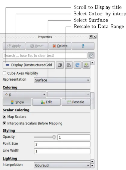
To view pressure, the user should go to the Displaypanel since it controls the visual repre-sentation of the selected module. To make a simple plot of pressure, the user should select the following, as described in detail in Figure2.4: selectSurfacefrom theRepresentation menu; select inColoring and Rescale to Data Range. Now in order to view the solution at t= 0.5 s, the user can use the VCR Controlsor Current Time Controlsto change the
Scroll to Display title
Select Color byinterpolated p Select Surface
Rescale to Data Range
Figure 2.4: Displaying pressure contours for the cavity case.
current time to 0.5. These are located in the toolbars below the menus at the top of the ParaView window, as shown in Figure 6.4. The pressure field solution has, as expected, a region of low pressure at the top left of the cavity and one of high pressure at the top right of the cavity as shown in Figure 2.5.
With the point icon ( ) the pressure field is interpolated across each cell to give a continuous appearance. Instead if the user selects the cell icon, , from the Color by menu, a single value for pressure will be attributed to each cell so that each cell will be denoted by a single colour with no grading.
A colour bar can be included by either by clicking theToggle Color Legend Visibilitybutton in the Active Variable Controls toolbar or the Coloring section of the Display panel. Clicking the Edit Color Mapbutton, either in theActive Variable Controlstoolbar or in the Coloring panel of the Displaypanel, the user can set a range of attributes of the colour bar, such as text size, font selection and numbering format for the scale. The colour bar can be located in the image window by drag and drop with the mouse.
ParaView defaults to using a colour scale of blue to white to red rather than the more common blue to green to red (rainbow). Therefore the first time that the user executes ParaView, they may wish to change the colour scale. This can be done by selecting the Choose Preset button (with the heart icon) in the Color Scale Editor and selecting Blue to Red Rainbow. After clicking theOKconfirmation button, the user can click theMake Default button so that ParaView will always adopt this type of colour bar.
If the user rotates the image, they can see that they have now coloured the complete geometry surface by the pressure. In order to produce a genuine contour plot the user should first create a cutting plane, or ‘slice’, through the geometry using the Slice filter as described in section6.1.6.1. The cutting plane should be centred at (0.05,0.05,0.005) and its normal should be set to (0,0,1) (click the Z Normalbutton). Having generated the cutting plane, the contours can be created using by the Contour filter described in section6.1.6. 2.1.4.2 Vector plots
Before we start to plot the vectors of the flow velocity, it may be useful to remove other modules that have been created, e.g. using the Slice and Contourfilters described above. These can: either be deleted entirely, by highlighting the relevant module in the Pipeline Browser and clicking Deletein their respective Properties panel; or, be disabled by toggling the eye button for the relevant module in thePipeline Browser.
We now wish to generate a vector glyph for velocity at the centre of each cell. We first need to filter the data to cell centres as described in section6.1.7.1. With thecavity.OpenFOAM module highlighted in the Pipeline Browser, the user should select Cell Centers from the Filter->Alphabetical menu and then clickApply.
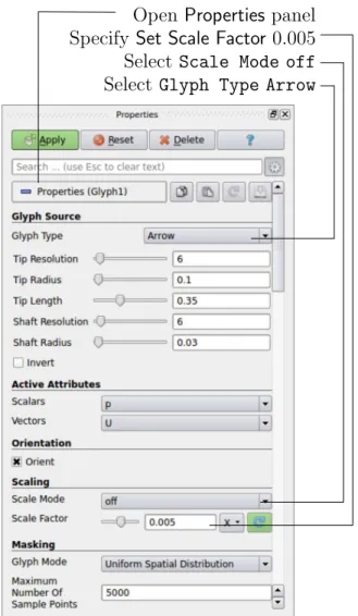
With theseCentershighlighted in thePipeline Browser, the user should then selectGlyph from the Filter->Common menu. The Properties window panel should appear as shown in Figure 2.6. Note that newly selected filters are moved to the Filter->Recent menu and are unavailable in the menus from where they were originally selected. In the resulting Properties panel, the velocity field,U, is automatically selected in the vectorsmenu, since it is the only vector field present. By default the Scale Mode for the glyphs will be Vector Magnitude of velocity but, since the we may wish to view the velocities throughout the domain, the user should instead select offandSet Scale Factorto 0.005. On clickingApply, the glyphs appear but, probably as a single colour, e.g. white. The user should colour the glyphs by velocity magnitude which, as usual, is controlled by setting Color by U in the
Open Properties panel Select Scale Mode off
Select Glyph Type Arrow
Specify Set Scale Factor0.005
Figure 2.6: Properties panel for the Glyph filter.
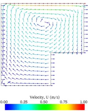
Display panel. The user should also select Show Color Legend in Edit Color Map. The output is shown in Figure 2.7, in which uppercase Times Roman fonts are selected for the Color Legendheadings and the labels are specified to 2 fixed significant figures by deselecting Automatic Label Formatand entering%-#6.2fin theLabel Formattext box. The background colour is set to white in the Generalpanel ofView Settings as described in section6.1.5.1. Note that at the left and right walls, glyphs appear to indicate flow through the walls. On closer examination, however, the user can see that while the flow direction is normal to the wall, its magnitude is 0. This slightly confusing situation is caused by ParaView choosing to orientate the glyphs in the x-direction when the glyph scaling off and the velocity magnitude is 0.
2.1.4.3 Streamline plots
Again, before the user continues to post-process in ParaView, they should disable modules such as those for the vector plot described above. We now wish to plot streamlines of velocity as described in section 6.1.8.
With thecavity.OpenFOAM module highlighted in the Pipeline Browser, the user should then selectStream Tracerfrom theFiltermenu and then clickApply. TheProperties win-dow panel should appear as shown in Figure 2.8. The Seedpoints should be specified along a High Resolution Line Source running vertically through the centre of the geometry, i.e. from (0.05,0,0.005) to (0.05,0.1,0.005). For the image in this guide we used: a point Resolution of 21; Maximum Step Length of 0.5; Initial Step Length of 0.2; and, Integration Direction BOTH. The Runge-Kutta 4/5 IntegratorType was used with default parameters.
On clicking Apply the tracer is generated. The user should then select Tube from the Filter menu to produce high quality streamline images. For the image in this report, we used: Num. sides 6; Radius0.0003; and, Radius factor 10. The streamtubes are coloured by velocity magnitude. On clicking Apply the image in Figure 2.9 should be produced.
2.1.5
Increasing the mesh resolution
The mesh resolution will now be increased by a factor of two in each direction. The results from the coarser mesh will be mapped onto the finer mesh to use as initial conditions for the problem. The solution from the finer mesh will then be compared with those from the coarser mesh.
2.1.5.1 Creating a new case using an existing case
We now wish to create a new case named cavityFine that is created from cavity. The user should therefore clone the cavity case and edit the necessary files. First the user should create a new case directory at the same directory level as the cavity case, e.g.
cd $FOAM RUN/tutorials/incompressible/icoFoam mkdir cavityFine
The user should then copy the base directories from the cavitycase intocavityFine, and then enter the cavityFine case.
Set Integration Direction to BOTH
Set Initial Step Length toCell Length0.01 Specify Line Source and set points and resolution Scroll to Properties title
Figure 2.8: Properties panel for the Stream Tracer filter.
cp -r cavity/system cavityFine cd cavityFine
2.1.5.2 Creating the finer mesh
We now wish to increase the number of cells in the mesh by using blockMesh. The user should open the blockMeshDictfile in an editor and edit the block specification. The blocks are specified in a list under the blocks keyword. The syntax of the block definitions is described fully in section 5.3.1.3; at this stage it is sufficient to know that following hex is first the list of vertices in the block, then a list (or vector) of numbers of cells in each direction. This was originally set to (20 20 1) for the cavity case. The user should now change this to (40 40 1) and save the file. The new refined mesh should then be created by running blockMesh as before.
2.1.5.3 Mapping the coarse mesh results onto the fine mesh
The mapFields utility maps one or more fields relating to a given geometry onto the cor-responding fields for another geometry. In our example, the fields are deemed ‘consistent’ because the geometry and the boundary types, or conditions, of both source and target fields are identical. We use the -consistent command line option when executing mapFields in this example.
The field data thatmapFieldsmaps is read from the time directory specified bystartFrom and startTime in the controlDict of the target case, i.e. those into which the results are being mapped. In this example, we wish to map the final results of the coarser mesh from case cavityonto the finer mesh of case cavityFine. Therefore, since these results are stored in the 0.5directory ofcavity, the startTimeshould be set to 0.5 s in thecontrolDictdictionary and startFrom should be set to startTime.
The case is ready to runmapFields. Typing mapFields -help quickly shows that map-Fields requires the source case directory as an argument. We are using the -consistent option, so the utility is executed from withing the cavityFine directory by
mapFields ../cavity -consistent
The utility should run with output to the terminal including:
Source: ".." "cavity" Target: "." "cavityFine" Create databases as time Case : ../cavity nProcs : 1
Source time: 0.5 Target time: 0.5 Create meshes
Source mesh size: 400 Target mesh size: 1600
Consistently creating and mapping fields for time 0.5 Creating mesh-to-mesh addressing ...
Overlap volume: 0.0001
interpolating p interpolating U End
2.1.5.4 Control adjustments
To maintain a Courant number of less that 1, as discussed in section 2.1.1.4, the time step must now be halved since the size of all cells has halved. Therefore deltaT should be set to to 0.0025 s in the controlDict dictionary. Field data is currently written out at an interval of a fixed number of time steps. Here we demonstrate how to specify data output at fixed intervals of time. Under the writeControl keyword in controlDict, instead of requesting output by a fixed number of time steps with thetimeStepentry, a fixed amount of run time can be specified between the writing of results using the runTime entry. In this case the user should specify output every 0.1 and therefore should set writeInterval to 0.1 and writeControltorunTime. Finally, since the case is starting with a the solution obtained on the coarse mesh we only need to run it for a short period to achieve reasonable convergence to steady-state. Therefore the endTimeshould be set to 0.7 s. Make sure these settings are correct and then save the file.
2.1.5.5 Running the code as a background process
The user should experience running icoFoam as a background process, redirecting the ter-minal output to a logfile that can be viewed later. From the cavityFine directory, the user should execute:
icoFoam > log & cat log
2.1.5.6 Vector plot with the refined mesh
The user can open multiple cases simultaneously in ParaView; essentially because each new case is simply another module that appears in the Pipeline Browser. There is one minor inconvenience when opening a new case inParaView because there is a prerequisite that the selected data is a file with a name that has an extension. However, in OpenFOAM, each case is stored in a multitude of files with no extensions within a specific directory structure. The solution, that the paraFoam script performs automatically, is to create a dummy file with the extension.OpenFOAM— hence, thecavitycase module is calledcavity.OpenFOAM. However, if the user wishes to open another case directly from within ParaView, they need to create such a dummy file. For example, to load thecavityFine case the file would be created by typing at the command prompt:
cd $FOAM RUN/tutorials/incompressible/icoFoam touch cavityFine/cavityFine.OpenFOAM
Now the cavityFine case can be loaded into ParaView by selecting Open from the File menu, and having navigated the directory tree, selecting cavityFine.OpenFOAM. The user can now make a vector plot of the results from the refined mesh in ParaView. The plot can be compared with the cavity case by enabling glyph images for both case simultaneously.
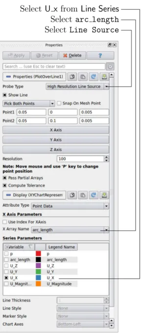
Selectarc length
Select U x from Line Series
Select Line Source
Figure 2.10: Selecting fields for graph plotting. 2.1.5.7 Plotting graphs
The user may wish to visualise the results by extracting some scalar measure of velocity and plotting 2-dimensional graphs along lines through the domain. OpenFOAM is well equipped for this kind of data manipulation. There are numerous utilities that do specialised data manipulations, and some, simpler calculations are incorporated into a single utilityfoamCalc. As a utility, it is unique in that it is executed by
foamCalc <calcType> <fieldName1 ... fieldNameN>
The calculator operation is specified in <calcType>; at the time of writing, the following
operations are implemented: addSubtract; randomise; div; components; mag; magGrad; magSqr; interpolate. The user can obtain the list of <calcType> by deliberately calling
one that does not exist, so that foamCalc throws up an error message and lists the types available, e.g.
>> foamCalc xxxx
Selecting calcType xxxx
unknown calcType type xxxx, constructor not in hash table Valid calcType selections are:
8 ( randomise magSqr magGrad addSubtract div mag interpolate components )
The components and mag calcTypes provide useful scalar measures of velocity. When “foamCalc components U” is run on a case, say cavity, it reads in the velocity vector field from each time directory and, in the corresponding time directories, writes scalar fields Ux, Uy and Uz representing the x,y and z components of velocity. Similarly “foamCalc mag U” writes a scalar field magU to each time directory representing the magnitude of velocity.
The user can run foamCalcwith thecomponents calcTypeon bothcavity and cavityFine cases. For example, for the cavity case the user should do into the cavity directory and execute foamCalc as follows:
cd $FOAM RUN/tutorials/incompressible/icoFoam/cavity foamCalc components U
The individual components can be plotted as a graph inParaView. It is quick, convenient and has reasonably good control over labelling and formatting, so the printed output is a fairly good standard. However, to produce graphs for publication, users may prefer to write raw data and plot it with a dedicated graphing tool, such as gnuplot orGrace/xmgr. To do this, we recommend using the sample utility, described in section 6.6 and section 2.2.3.
Before commencing plotting, the user needs to load the newly generated Ux, Uy and Uz fields into ParaView. To do this, the user should click the Refresh Times at the top of the Properties panel for the cavity.OpenFOAM module which will cause the new fields to be loaded into ParaView and appear in the Volume Fields window. Ensure the new fields are selected and the changes are applied, i.e. click Apply again if necessary. Also, data is interpolated incorrectly at boundaries if the boundary regions are selected in the Mesh Parts panel. Therefore the user should deselect the patches in the Mesh Parts panel, i.e.movingWall,fixedWall and frontAndBack, and apply the changes.
Now, in order to display a graph in ParaView the user should select the module of interest,e.g.cavity.OpenFOAMand apply thePlot Over Linefilter from theFilter->Data Analysismenu. This opens up a newXY Plotwindow below or beside the existing 3D View window. APlotOverLinemodule is created in which the user can specify the end points of the line in the Properties panel. In this example, the user should position the line vertically up the centre of the domain,i.e. from (0.05,0,0.005) to (0.05,0.1,0.005), in thePoint1and Point2 text boxes. TheResolution can be set to 100.
On clicking Apply, a graph is generated in the XY Plot window. In the Display panel, the user should set Attribute Mode to Point Data. The Use Data Array option can be selected for the X Axis Data, taking the arc length option so that the x-axis of the graph represents distance from the base of the cavity.
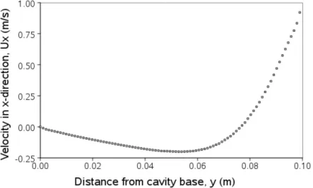
Figure 2.11: Plotting graphs in paraFoam.
The user can choose the fields to be displayed in the Line Series panel of the Display window. From the list of scalar fields to be displayed, it can be seen that the magnitude and components of vector fields are available by default, e.g. displayed as U X, so that it was not necessary to create Ux using foamCalc. Nevertheless, the user should deselect all series except Ux (or U x). A square colour box in the adjacent column to the selected series indicates the line colour. The user can edit this most easily by a double click of the mouse over that selection.
In order to format the graph, the user should modify the settings below the Line Series panel, namelyLine Color,Line Thickness,Line Style,Marker StyleandChart Axes. Also the user can click one of the buttons above the top left corner of theXY Plot. The third button, for example, allows the user to controlView Settingsin which the user can set title and legend for each axis, for example. Also, the user can set font, colour and alignment of the axes titles, and has several options for axis range and labels in linear or logarithmic scales.
Figure2.11is a graph produced using ParaView. The user can produce a graph however he/she wishes. For information, the graph in Figure 2.11was produced with the options for axes of: Standard type of Notation; Specify Axis Range selected; titles in Sans Serif 12 font. The graph is displayed as a set of points rather than a line by activating the Enable Line Series button in the Display window. Note: if this button appears to be inactive by being “greyed out”, it can be made active by selecting and deselecting the sets of variables in the Line Seriespanel. Once the Enable Line Seriesbutton is selected, the Line Style and Marker Style can be adjusted to the user’s preference.
2.1.6
Introducing mesh grading
The error in any solution will be more pronounced in regions where the form of the true solution differ widely from the form assumed in the chosen numerical schemes. For example a numerical scheme based on linear variations of variables over cells can only generate an exact solution if the true solution is itself linear in form. The error is largest in regions where the true solution deviates greatest from linear form,i.e. where the change in gradient is largest. Error decreases with cell size.
up any problem. It is then possible to anticipate where the errors will be largest and to grade the mesh so that the smallest cells are in these regions. In the cavity case the large variations in velocity can be expected near a wall and so in this part of the tutorial the mesh will be graded to be smaller in this region. By using the same number of cells, greater accuracy can be achieved without a significant increase in computational cost.
A mesh of 20×20 cells with grading towards the walls will be created for the lid-driven cavity problem and the results from the finer mesh of section 2.1.5.2 will then be mapped onto the graded mesh to use as an initial condition. The results from the graded mesh will be compared with those from the previous meshes. Since the changes to theblockMeshDict dictionary are fairly substantial, the case used for this part of the tutorial, cavityGrade, is supplied in the $FOAM RUN/tutorials/incompressible/icoFoam directory.
2.1.6.1 Creating the graded mesh
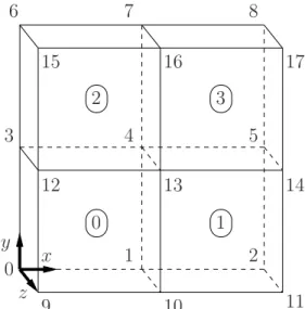
The mesh now needs 4 blocks as different mesh grading is needed on the left and right and top and bottom of the domain. The block structure for this mesh is shown in Figure 2.12. The
0 z x y 3 4 5 6 7 8 1 2 17 15 9 10 11 16 12 13 14 0 1 2 3
Figure 2.12: Block structure of the graded mesh for the cavity (block numbers encircled). user can view the blockMeshDict file in the system (or constant/polyMesh) subdirectory of cavityGrade; for completeness the key elements of the blockMeshDictfile are also reproduced below. Each block now has 10 cells in the x and y directions and the ratio between largest and smallest cells is 2.
17 convertToMeters 0.1; 18 19 vertices 20 ( 21 (0 0 0) 22 (0.5 0 0) 23 (1 0 0) 24 (0 0.5 0) 25 (0.5 0.5 0) 26 (1 0.5 0) 27 (0 1 0) 28 (0.5 1 0) 29 (1 1 0) 30 (0 0 0.1) 31 (0.5 0 0.1) 32 (1 0 0.1) 33 (0 0.5 0.1) 34 (0.5 0.5 0.1) 35 (1 0.5 0.1)
36 (0 1 0.1) 37 (0.5 1 0.1) 38 (1 1 0.1) 39 ); 40 41 blocks 42 ( 43 hex (0 1 4 3 9 10 13 12) (10 10 1) simpleGrading (2 2 1) 44 hex (1 2 5 4 10 11 14 13) (10 10 1) simpleGrading (0.5 2 1) 45 hex (3 4 7 6 12 13 16 15) (10 10 1) simpleGrading (2 0.5 1) 46 hex (4 5 8 7 13 14 17 16) (10 10 1) simpleGrading (0.5 0.5 1) 47 ); 48 49 edges 50 ( 51 ); 52 53 boundary 54 ( 55 movingWall 56 { 57 type wall; 58 faces 59 ( 60 (6 15 16 7) 61 (7 16 17 8) 62 ); 63 } 64 fixedWalls 65 { 66 type wall; 67 faces 68 ( 69 (3 12 15 6) 70 (0 9 12 3) 71 (0 1 10 9) 72 (1 2 11 10) 73 (2 5 14 11) 74 (5 8 17 14) 75 ); 76 } 77 frontAndBack 78 { 79 type empty; 80 faces 81 ( 82 (0 3 4 1) 83 (1 4 5 2) 84 (3 6 7 4) 85 (4 7 8 5) 86 (9 10 13 12) 87 (10 11 14 13) 88 (12 13 16 15) 89 (13 14 17 16) 90 ); 91 } 92 ); 93 94 mergePatchPairs 95 ( 96 ); 97 98 // ************************************************************************* //
Once familiar with the blockMeshDictfile for this case, the user can execute blockMeshfrom the command line. The graded mesh can be viewed as before using paraFoam as described in section 2.1.2.
2.1.6.2 Changing time and time step
The highest velocities and smallest cells are next to the lid, therefore the highest Courant number will be generated next to the lid, for reasons given in section 2.1.1.4. It is therefore useful to estimate the size of the cells next to the lid to calculate an appropriate time step for this case.
When a nonuniform mesh grading is used, blockMesh calculates the cell sizes using a geometric progression. Along a length l, if n cells are requested with a ratio of R between the last and first cells, the size of the smallest cell, δxs, is given by:
δxs =l
r−1
αr−1 (2.5)
where r is the ratio between one cell size and the next which is given by:
r=Rn−11 (2.6) and α= ( R for R >1, 1−r−n +r−1 for R <1. (2.7)
For the cavityGrade case the number of cells in each direction in a block is 10, the ratio between largest and smallest cells is 2 and the block height and width is 0.05 m. Therefore the smallest cell length is 3.45 mm. From Equation2.2, the time step should be less than 3.45 ms to maintain a Courant of less than 1. To ensure that results are written out at convenient time intervals, the time step deltaT should be reduced to 2.5 ms and the writeInterval set to 40 so that results are written out every 0.1 s. These settings can be viewed in the cavityGrade/system/controlDict file.
The startTime needs to be set to that of the final conditions of the case cavityFine, i.e.0.7. Since cavity and cavityFine converged well within the prescribed run time, we can set the run time for case cavityGrade to 0.1 s,i.e. the endTimeshould be 0.8.
2.1.6.3 Mapping fields
As in section 2.1.5.3, use mapFields to map the final results from case cavityFine onto the mesh for case cavityGrade. Enter the cavityGrade directory and executemapFields by:
cd $FOAM RUN/tutorials/incompressible/icoFoam/cavityGrade mapFields ../cavityFine -consistent
Now run icoFoam from the case directory and monitor the run time information. View the converged results for this case and compare with other results using post-processing tools described previously in section 2.1.5.6 and section 2.1.5.7.
2.1.7
Increasing the Reynolds number
The cases solved so far have had a Reynolds number of 10. This is very low and leads to a stable solution quickly with only small secondary vortices at the bottom corners of the cavity. We will now increase the Reynolds number to 100, at which point the solution takes a noticeably longer time to converge. The coarsest mesh in casecavity will be used initially. The user should make a copy of the cavity case and name itcavityHighRe by typing:
cd $FOAM_RUN/tutorials/incompressible/icoFoam cp -r cavity cavityHighRe