Economic and environmental effects of border tax adjustments

(1)

econ

stor

www.econstor.eu

Der Open-Access-Publikationsserver der ZBW – Leibniz-Informationszentrum Wirtschaft The Open Access Publication Server of the ZBW – Leibniz Information Centre for Economics

Nutzungsbedingungen:

Die ZBW räumt Ihnen als Nutzerin/Nutzer das unentgeltliche, räumlich unbeschränkte und zeitlich auf die Dauer des Schutzrechts beschränkte einfache Recht ein, das ausgewählte Werk im Rahmen der unter

→ http://www.econstor.eu/dspace/Nutzungsbedingungen nachzulesenden vollständigen Nutzungsbedingungen zu vervielfältigen, mit denen die Nutzerin/der Nutzer sich durch die erste Nutzung einverstanden erklärt.

Terms of use:

The ZBW grants you, the user, the non-exclusive right to use the selected work free of charge, territorially unrestricted and within the time limit of the term of the property rights according to the terms specified at

→ http://www.econstor.eu/dspace/Nutzungsbedingungen By the first use of the selected work the user agrees and declares to comply with these terms of use.

zbw

Leibniz-Informationszentrum Wirtschaft Leibniz Information Centre for Economics

Peterson, Everett B.; Schleich, Joachim

Working Paper

Economic and environmental effects of

border tax adjustments

Working paper sustainability and innovation, No. S1/2007 Provided in cooperation with:

Fraunhofer-Institut für System- und Innovationsforschung (ISI)

Suggested citation: Peterson, Everett B.; Schleich, Joachim (2007) : Economic and

environmental effects of border tax adjustments, Working paper sustainability and innovation, No. S1/2007, urn:nbn:de:0011-n-559250 , http://hdl.handle.net/10419/28514

(2)

Working Paper Sustainability and Innovation No. S 1/2007 (Revised Version October 2007)

Everett B. Peterson Joachim Schleich

Economic and Environmental Effects of Border Tax Adjustments

Fraunhofer ISI Institute Systems and nnovation Research I

(3)

Abstract

Taxing imports from regions which are not subject to climate policy and subsidi-zing exports into these regions have recently been proposed to address presu-med negative effects of the EU Emissions Trading Scheme (EU ETS) on in-dustry competitiveness and carbon leakage. This paper analyzes the economic and environmental effects of alternative border tax adjustment (BTA) mecha-nisms using an extended version of the GTAP-E model that explicitly includes domestic trade and transport margins. The BTAs are imposed on regions which have not committed to emission targets under the Kyoto Protocol or which failed to ratify the Kyoto Protocol. The analyses distinguish between effects of the BTAs on the EU15 countries and on the rest of the EU (REU). Likewise, the analyses single out the effects of climate policy with and without BTAs on do-mestic output changes which are due to changes in import competition and ex-port competitiveness. Implementing a BTA whose power is equal to the percen-tage change in production costs in the energy-intensive sectors in the EU has different impacts for those sectors in the EU15 countries compared with the REU countries. In the EU15, the BTA effectively neutralizes import competition in the energy-intensive sectors while enhancing the export competitiveness of these sectors. Conversely, in the REU, the BTA is not effective in neutralizing increased import competition or decreased export competitiveness because the majority of trade by the REU is with countries/regions that are not included in the BTA. Overall, implementing a BTA has little effect on the marginal abate-ment costs of achieving the emission reductions in the Kyoto Protocol and does little in reducing carbon leakage.

(4)

Economic and Environmental Effects of Border Tax Adjustments I

Figures

Page Figure 1: Structure of Production in GTAP-E Model ... 5 Figure 2: Structure of Domestic Marketing Margins... 7

Tables

Page

Table 1: Regional/country Aggregation ... 12 Table 2: Commodity/sector Aggregation ... 13 Table 3: Production, Margin, and Trade Elasticities of

Substitution... 14 Table 4. Simulation Results for Implementation of Kyoto

Protocol ... 18 Table 5. Change in EU Output Attributable to Trade ... 20 Table 6. Simulation Results for EU Implementation of Border

(6)

Economic and Environmental Effects of Border Tax Adjustments 1

1 Introduction

Partial implementation of environmental policies in some regions will not lead to a cost-efficient outcome in case of transnational externalities. Yet such policies are observed in the context of international climate policy. In particular, in the Kyoto Protocol only so called Annex B countries have committed to reduce greenhouse gases by approximately 5.2% from the 1990/1995 base year levels during the first commitment period of 2008-2012. Even though the United States and Australia refused to ratify the Kyoto Protocol, adopting members implemen-ted the agreement in 2005. In the same year, the European Union launched an EU-wide trading scheme (EU ETS) for CO2-emissions generated by companies in the energy industry and other carbon-intensive industry sectors as its key climate change policy instrument. Approximately 12,000 installations are cur-rently covered by the EU ETS and account for nearly 45% of total CO2 -emissions, and about 30% of all greenhouse gases in the EU (CEC 2005). The purpose of the EU ETS is to allow EU Member States to achieve their Kyoto greenhouse gas emission targets at minimum cost. However, this partial imple-mentation of emissions trading may result in competitive distortions for carbon-intensive companies like producers of cement or steel in the EU. Since partici-pating in the EU ETS increases the marginal production costs, depending on the carbon intensity of the production process and the price for EU allowances, companies from these sectors which export to regions that have not implemen-ted climate policy would be disadvantaged since the additional (opportunity) costs may generally not be passed on. Likewise, EU companies that face import competition from companies in regions that have not implemented climate change policies would also be at a competitive disadvantage.1_{Because of}

the-se changes in competitiveness, the production of energy-intensive products may shift to regions without climate change policies. This would lead to carbon leakage and a smaller reduction in global CO2 emissions if firms in these count-ries employ less carbon efficient production processes. As a consequence, BTAs may also allow regions to take leadership in terms of climate policy. For example, the EU has committed to reduce greenhouse gas emissions by 2020 by 20%, even if there was no Post-Kyoto agreement.

1 Since in the EU ETS at least 90% of allowances have to be allocated for free for the period 2008-2012, actual costs to companies would be lower than the opportunity costs. However, competitiveness is determined by the marginal costs, which under ideal conditions do not depend on whether allowances are allocated for free or auctioned off.

(7)

2 Economic and Environmental Effects of Border Tax Adjustments

To address these concerns, border tax adjustments (BTA) have recently been proposed by academics (e.g. Ismer and Neuhoff 2004, Grubb and Neuhoff 2006, Stiglitz 2006), industry associations (e.g. CEMBUREAU), and politicians. The proposed border adjustments would tax imports from regions that have not implemented climate change policies and subsidize exports to those regions. The tax and subsidy rates would correspond to the additional (opportunity) costs imposed on like commodities produced in the EU. Thus, the higher the carbon tax (implied through emission trading), the higher will be the tax burden on imported commodities and the higher the subsidy on EU exports.2_Current

proposals for a US national greenhouse gas trading system include provisions which are similar to a BTA and are meant to induce participation of those count-ries in a global effort to reduce greenhouse gas emissions which failed to take appropriate measures. According to the Lieberman-Warner America’s Climate Security Act of 2007, importers of greenhouse-gas-intensive manufactured pro-ducts from such countries would have to submit emissions allowances of a va-lue that matches that of the allowances domestic manufacturers pay under the US system.3

In practice, at least three types of problems may arise with the implementation of a BTA mechanism. First, because of information costs and information a-symmetry, it may be difficult to determine the appropriate level of the import ta-riffs and export subsidies that offset the loss of competitiveness. Ideally, the power of the BTA would be set equal to the percentage change in costs from implementing climate change policies. However, this may be difficult to measure and there would be incentives for firms to include cost increases not associated with climate change policies to obtain larger tariffs and export subsidies. Se-cond, the set of commodities which would be subject to the BTA have to be de-fined. Annex 1 of the EU Emissions Trading Directive lists the types of installati-ons which are directly covered by the EU ETS. However, since the EU ETS not only increases prices of final commodities, but also of intermediate commodities such as electricity, the competitiveness of companies which do not participate in the EU ETS but intensively use these intermediates, may also be affected nega-tively. Sectors indirectly affected by the EU ETS include, in particular, the alu-minum and large parts of the chemical industry. Third, it is doubtful whether

2 Other remedies discussed to address incomplete regulatory coverage include output-based allocation of allowances or rebate systems (see Demailly and Quirion 2006, Demailly and Quirion 2007b, Fischer (forthcoming), or Bernard et al. 2007).

(8)

BTA would be compatible with current WTO/GATT rules (e.g., van Asselt and Biermann 2007). Notably, Ismer and Neuhoff (2004) argue that a BTA would be allowed under WTA rules if it is based on emissions of best-available technolo-gies (BAT).

In this paper we analyze the economic and environmental effects of the EU implementing a BTA policy employing a static version of the GTAP-E model that also includes domestic trade and transport margins. Such margins are particu-larly relevant for some of the sectors included in the EU ETS such as cement or lime producers. Peterson and Lee (2005) have shown that the impact of energy taxes on prices and emissions may be significantly overstated if the domestic trade and transport margins are not explicitly modeled. The power of the BTA is set equal to the percentage change in costs for sectors that are subject to the BTA, with the BTA being imposed on two alternative sets of industries: those industries directly participating in the EU ETS and those industries directly or indirectly affected by the EU ETS.

This paper extends existing applied general equilibrium (AGE) based analyses of the EU ETS (including Klepper and Peterson 2006, or Kemfert et al. 2006) which do not allow for BTAs (and not for transport margins), and do not distin-guish between effects on the EU15 and the REU countries. It complements e-xisting analyses on BTAs for selected sectors such as steel and cement based on partial-equilibrium models (including Demailly and Quirion forthcoming, De-mailly and Quirion 2007, and Mathiesen and Mæstad 2004). Finally, the paper distinguishes the effects on domestic output which result from changes in import and export competitiveness.

(9)

2 Model

Description

The model employed is an extended version of the static GTAP-E Model (Burniaux and Truong 2002). This model is based on the perfectly competitive, multi-region, multi-sector GTAP model (Hertel and Tsiagas 1997). Because the GTAP-E explicitly models substitution possibilities between energy inputs and between energy and capital; and also tracks CO2 emissions, it has been frequently used in the analysis of climate change policies (e.g. Kremers et al. 2002, Nijkamp et al. 2005 or Kemfert et al. 2006). Our model extends the GTAP-E model by including domestic trade and transport margins.

2.1 Regional Household Demand

In each region, there is a single aggregate household that represents the con-sumption side of the model. This regional aggregate household collects all of the factor income and tax receipts and spends this income on private consumption of goods and services, government consumption, and savings. The utility function for the aggregate regional household consists of two levels. At the top-level, a Cobb-Douglas utility function is specified such that shares of private consumption, go-vernment consumption, and savings remain constant. At the second-level, a non-homothetic Constant Difference Elasticity of substitution (CDE) utility function is used to represent preferences for private consumption. Also at the second-level, a Cobb-Douglas utility function is used to represent preferences for government con-sumption.

2.2 Production

Similar to the GTAP-E model, a nested Constant Elasticity of Substitution (CES) pro-duction structure, as illustrated in Figure 1, is specified in the model. Each sub-nest in the production structure represents the potential for substitution between individual or composite inputs. Each composite input is composed of the commodities at the next lower level in the tree structure of Figure 1. Beginning at the top of the producti-on structure, firms produce output by using nproducti-on-energy intermediate inputs and a primary factor composite (or value added). Typically, the elasticity of substitution between the primary factor composite and non-energy intermediate inputs (σT) is assumed to equal zero. This implies a constant per-unit-of-output input use of all non-energy intermediate inputs and the primary factor composite. The primary factor composite is composed of land, skilled labor, unskilled labor, natural resources, and a capital-energy composite with a constant elasticity of substitution (σVA) between them.

(10)

Econo

mic a

nd

Environme

ntal Effects of Border T

ax Adjustme

nts

5

Figure 1:

Structure of

Production in GTAP-E Model

Output Intermediate Inputs (non-energy) Value Added Land Skilled Labor Unskilled Labor Natural _Resource Capital-Energy Composite Capital Energy Electricity Non-Electricity Coal Non-Coa l Petroleum Products Gas Oil

(11)

Econo

Within the capital-energy co sibilities: (a

mic and Environmental Effects of Border Tax Adjustments 6

mposite, there are three inter-fuel substitution pos-) electricity versus non-electricity composite (σELY); (b) coal versus non-coal composite (σCOAL); and (c) between oil, gas, and petroleum products (σFU). For example, producers may substitute coal for non-coal fuel (a composi-te of oil, gas and petroleum products) when coal becomes more expensive than non-coal fuels. Firms may also substitute the energy composite (σKE) for capital when the aggregate energy price decreases relative to the capital rental rate. As pointed out by Burniaux and Truong (2002), the advantages to this specifica-tion is that it allows f r substituspecifica-tion between fuels and the potential for capital and energy to be either substitutes or complements, depending on the values of the elasticities o bstitution chosen.

2.3 Incorporating Domestic Margins

Domestic margins, which drive a we purchaser

pri-ces, have been incorporated into per, we follow the specification of

hin (2006), and Peterson (2006). This approach specifies a nested CES structu-re shown in Figustructu-re 2. At the top of this structustructu-re is a composite commodity that is pu sed by the private household, government household, or firms. Similar to the GTAP-E model, the composite commodity is a combination of the margin inclus omposite imported commodity and a margin inclusive domestic commodity (see Level 3 of Figure 2), where σD is the elasticity of substitution between the composite import and the composite domestic commodity. Note that the composite commodities include domestic trade and transportation mar-gins. At Level 2, the composite imported commodity and the domestically pro-duced commodity are combined with a composite marketing service. Based on the work of Holloway (1989) and Wohlgenant (1989), the potential for substituti-on between the composite comm composite marketing service is de-noted as σpt. As shown in Level 1, the composite marketing service is itself a CES aggregate of all trade and transportation services needed to get the good from the producer to the purchaser. The constant elasticity of substitution σpm governs the degree of substitutability ween individual marketing services, such as land and air transport, as relative prices vary. Note that levels 1 and 2 do not exist in the GTAP-E model.

o f su

dge between producer and

omestic margins used by Bradford and AGE models in a v

d

ariety of ways. In this

pa-rcha ive c

odity and

(12)

mic a

nd

Environme

ax Adjustme

nts

7

Level 1 Level 2 Level 3

Structure of Do

mestic Marketing Margins

Composite Commodity

Margin Inclusive Import

Margin Inclusive Dom

estic Composite Imported Commodity Domestic _Commodity Composite Marketing Service Trade Composite Marketing Service Trade Transportation

σ

pm

σ

pt

σ

pt

σ

D

σ

pm Transportation Econo Figure 2:

(13)

In addition to applying domestic margins on the purchases of all agents in the model, domestic margins are also applied on all commodities that are exported.

two-level ne omestic trade

At the top level, this combined with exports to

create the f.o.b. expor

2.4 CO

2

The emission of CO sumed to be

gas, and petroleum and coal pr 2 emissions

from energy commodity e in region r is specified as:

( )

(

)

( )

(

( )

2( , ) , , , , , , , , j pro m C e V e CO r e QFD e j r QFM e j r QPD e r V e Q e QPM e r QGD e r e r ∈ ⎡ ⎤ ⎡ ⎤ ⎧ =_⎢ _{⎥ ⎢} _⎥_⎨ ⎡_⎣ + ⎤_⎦+ + ⎩ ⎣ ⎦ ⎣ ⎦ + +

∑

₍₁₎

where CO2 is defined as millions of metric tons (MT) emitted; (C/V) is the a-mount of CO2 ion tons of oil equivalent); (V/Q) is the mtoe per unit of energy commodity; QFD QFM are the level of domestic and imported intermediate inputs; QPD and M are the level of domestic and imported energy commodities purchased by the private household; and QGD

and QGM are the level of domestic and im

urcha-sed by the government. So the terms (C/V

of the energy commodity into the level of CO emissions. The percentage chan-ge in CO

These margins represent domestic trade and transport services utilized to get the commodity from the producer to the port of departure. Similar to Figure 2, a

sted CES structure is utilized. At the bottom level, d

and transport services are combined to create a composite marketing service. composite marketing service is

t composite commodity.

Emissions

2 per unit of energy commodities used is as

constant across users and regions, but varies by energy commodity (coal, oil, oducts). Formally, the level of CO

(

)

_

d com

QGM

}

emissions per mtoe (mill

and

QP

ported energy commodities p )(V/Q) convert the physical quantities

2 2 emissions is:

(

)

(

)

(

)

(

)

( )

2( 2( , ) , * * , , , * , , , , * , , * , , j

CO r gco r e EDINT r qfd EMINT e j qfm e j r EDHH e r e r E e r qpm e r EDGV e r qgd e r EMGV e r qgm e r , )*e

( )

, , e j r MHH , e j qpd , ,r = ⎡_⎣ + ⎤_⎦+ + + +

∑

(2) where is the percentage change in CO2 emissions; EDINT, EMINT, EDHH HH, EDG EMGV are the amount of CO2 emitted from

do-gco2

(14)

mestic and imported intermediate energy inputs, domestic and imported energy commodities consumed by the private household, and domestic and imported energy commodities consumed by the government households; and qfd, qfm,

qpd, qpm, qgd, qgm, are the percentage changes in the use of energy commo-dities by firms, private households, and the government.

2.5 Carbon Tax and Emission Trading

A carbon tax, both on a real and nominal basis, is used to represent the margi-nal abatement costs in the model. The level of the carbon tax is endogenously

epends on the level of quantitative restrictions on

(3) where NCTAX(r) and RCTAX(r) are the nominal and the real carbon tax rat

region r and GDPIND(r) is the GDP deflator of region r. The change in the no-minal tax rate is specified as:

determined in the model and d

CO2 emissions in the Annex B countries. When emission trading is permitted, one may interpret the carbon tax as the value of CO2 permits.

In levels form, the nominal carbon tax is specified as:

( ) ( )* ( )

NCTAX r = GDPIND r RCTAX r ,

e for

( )

*

( )

+0.01*

( )

* ( )

nctax r = GDPIND r rctax r NCTAX r pgdp r

, (4) where nctax(r) and rctax(r) are the changes in the nominal and the real carbon

tax rates for region r and pgdp(r) is the percentage change in the GDP deflator in region r.

When a group of countries join an emissions trading scheme, the marginal aba-tement costs are equalized across countries through the trading of CO2 emissi-on permits. In terms of equatiemissi-ons (3) and (4), this implies that NCTAX(r) is e-qualized in all participating countries. Formally, the value of traded emissions permits is specified in the model as:

( )

2 2 2 *

DVCO TRA r =⎡_⎣CO Q r −CO T r ⎤_⎦ NCTAX r( )

(5) where CO2Q(r) is the CO2 emissions quota for region r; CO2T(r) is the total CO2

emissions of region r; and DVCO2TRA(r) is the dollar value from CO2 emissions trading of region r. If DVCO2TRA(r) is negative, country r is buying emissions

(15)

permits, as it emits more than its allocated quota. If DVCO2TRA(r) is positive, country r is selling emissions permits, as it emits less than its allocated quota. The change in the dollar value of emissions trading is specified as:

( )

2 0.01* * 2 * 2 - 2 * 2

dvco tra r = NCTAX r ⎡_⎣CO Q r gco q r CO T r gco t r ⎤+

( )

* 2

( )

- 2

( )

,

nctax r CO Q r CO T r

⎦

⎡ ⎤

⎣ ⎦ ₍₆₎

r effects on the purchaser price for a given level of the carbon

achieve a comparable level of emission abatement. In addition, accounting for domestic transport costs is particularly relevant for the cement and lime indust-where dvco2tra(r) is the change in dollar value from CO2 emissions trading; gco2q(r) and gco2t(r) are the percentage changes in the CO2 emissions quota and total CO2 emissions.

The inclusion of domestic trade and transport margins in the model creates a wedge between producer and purchaser prices. Compared to models that do not account for domestic margins, this leads to smalle

tax. Thus, a larger carbon tax is needed to

ries that are included in the EU ETS. Trade in these industries is restricted to about 200 km radius because of transport costs (Demailly and Quirion, forthco-ming).

(16)

3 Data and Model Aggregation

The data used to implement the model is based on version 6.0 the GTAP data base. Peterson (2006) has developed a domestic margin inclusive version of the GTAP version 6 data base that contains information on trade and transpor-tation margins for all intermediate input purchases, purchases by households, and purchases by governments of domestically produced and imported modities. It also includes all domestic trade and transport margins required to

e, Finland, France, Hungary, Italy, Japan, Malta, the Netherlands, Poland, Portugal, Spain, Sweden, Slovakia, Slovenia, the United

(ROA), China and India (CHIND), Japan, (JPN), the United States (US), Rest of Central and South America (CSAM), EU15, Rest of European Union (REU), Rest of Eastern Europe and former Soviet Union, (REFSU), and Middle East and Africa (MEAF). The European Union is disaggregated into two regions because of differences in CO2 emissions, product carbon content, and reduction targets between the EU15 and rest of the member states. Japan is identified separately from the rest of the Annex B countries due its larger amount of CO2 emissions. The United States, Australia, and China and India are identified as separate regions because these are relatively large CO2 emitters and/or failed to ratify the Kyoto Protocol. All other composite regions are defined based on geographic proximity. Table 1 provides a detailed description of the regional aggregation.

com-get exports to the port of departure. This margin data is based on data from the Input-Output accounts of 22 countries (Australia, Austria, Belgium, Denmark, Estonia, Germany, Greec

Kingdom, and the United States). For regions where no margin data are avail-able, average margin shares are used (see Peterson, 2006, for more details). The levels of initial CO2 emissions for each region by energy commodities are based on the GTAP version 6 energy data base. The base year of the data used in this analysis is 2001.4

An eleven region and seventeen commodity aggregation is used in this paper. The eleven regions are Australia (AUS), Rest of Annex B countries (ROB), Rest of Asia

4 Because the base year is 2001, the GTAP version 6.0 data base contains trade barriers between some of the new EU member states, such as Poland, and other EU member sta-tes. These barriers are removed in an initial simulation that creates an updated data base with no trade barriers between EU member states. We use this updata data as the base for all simulations conducted in this paper.

(17)

Table 1: Regional/country Aggregation

Region Description GTAP Regions Emission Target* EU15 EU15 aut, bel, dnk, fin, fra, deu, gbr,

grc, irl, ita, lux, nld, prt, esp, swe

-6.9% REU Rest of EU bgr, cyp, cze, hun, mlt, pol,

rom, svk, svn, est, lva, ltu 33.0%

JPN Japan jpn -12.7%

REFSU Rest of Eastern Europe &

Former Soviet Union xer, alb, hrv, rus, xsu

ROB Rest of Annex B can, che, xef, nzl -25.1% AUS Australia aus

CHIND China and India chn, hkg, ind

MEAF Middle East & Africa tur, xme, mar, tun, xnf, bwa, zaf, xsc, mwi, moz, tza, zmb, zwe, xsd, mdg, uga, xss

CSAM Central & South America mex, xna, col, per, ven, xap, arg, bra, chl, ury, xsm, xca, xfa, xcb

ROA Rest of Asia xoc, kor, twn, xea, idn, mys, phl, sgp, tha, vnm, xse, bgd, lka, xsa

US United States usa

* Based on Ziesing (2006). Total emission reduction of 5.2% across all Annex B regions

The seventeen commodities/sectors in the model are agriculture (agr), food, coal, oil, gas, other natural resources (onres), paper products (ppp), petroleum and coal products (p_c), chemical, rubber, plastic products (crp), other mineral products (nmm), ferrous metals (i_s), other metals (nfm), other manufacturing (oman), electricity (ely), trade (trd), transport (trans), and services (serv). The sectors ppp, p_c, nmm, i_s, and ely are the GTAP sectors that most closely cor-respond to those covered by the EU ETS. The sectors crp and nfm are also re-latively larger users of energy and may be included in a BTA policy. Coal, oil, and gas represent the extraction of the fossil based energy commodities. Trade and transports sectors are identified separately because of their use in provi-ding domestic margin services and relatively large use of petroleum products by the transport sector. Food, agr, onres, and serv are composite commodities that represent the remaining sectors. Table 2 provides a detailed description of the commodity/sector aggregation.

(18)

Table 2: Commodity/sector Aggregation

Sectors Sector Description GTAP

agr Agriculture pdr, wht, gro, v_f, osd, c_b, pfb, o oap, rmk, wol cr, ctl, food Food cmt, omt, vol, mil, pcr, s

coa gr, ofd, b_t coal Coal oil urces mn ucts ppp al products stic pr nmm* Other mineral products nfm** Other metal products

cturing p, mvh, otn, ele, ely* Electricity ely

trd ran

oil Oil

gas Gas gas, gdt onres Other natural reso frs, fsh, o

ppp* Paper prod

p_c* Petroleum and co p_c crp** Chemicals, rubber, pla oducts crp

nmm

i_s* Ferrous metals i_s nfm

oman Other manufa tex, wap, lea, lum, fm ome, omf

trd Trade

t s Transport otp, wtp, atp

serv Services cmn, ofi, isr, obs, ros, osg, dwe * ETS sector

** ETS affected sector

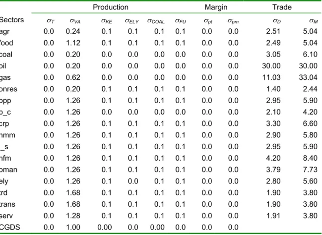
The production, margin, and trade elasticities of substitution utilized in the mo-del are listed in table 3. No substitution is allowed between non-energy interme-diate inputs and value-added (σT). We also assume fixed margins and set the values of σpm and σpt equal to zero. The elasticities of substitution among the components of value-added (σVA) are set equal to those values in the GTAP version 6.0 data base. Because we believe that the elasticities of substitution between energy and capital (σKE), electricity and non-electricity (σELY), and coal and non-coal (σCOAL), and between non-coal energy intermediate inputs (σFU) in Burniaux and Truong (2002) are too large for the short to intermediate run, we consider alternative scenarios where the values of these parameters are set equal to 0.1 and 0.25 respectively.5_{Following Burniaux and Truong (2002), we}

o not allow for substitution among energy commodities or between energy and

d

In a recent micro-panel econometric study of industrial companies, Arberg and Bjørner (2007) find that electricity and other energy inputs are complements with capital rather than substitutes.

(19)

capital in the mining and refining of fossil fuels (i.e., σKE, σELY, σCOAL, and σFU are set equal to zero for coal, oil, gas, and p_c). We also do not allow substituti-o etween e nd non-electricity in

the elasticities of substitution between domestic and the composite imported

commodity (σ between imported commo lues

in the GTAP v6 data base with the exception of oil, where the trade elasticities are set equal to 30, reflecting the belief that crude oil is a more homogeneous commodity.

Table 3: argin, and Trade Elasticities of Substitution

Margin Trade

n b lectricity a the electricity (ely) sector. Finally, D) and dities (σM) are equal to the va

Production, M

Production

Sectors σT σVA σKE σELY σCOAL σFU σpt σpm σD σM

agr 0 0.1 0.1 0.0 0.0 2.51 5.04 0 0.1 0.1 0.0 0.0 2.49 5.04 0 0.0 0.0 oil 0.0 0.20 0.0 0.0 0.0 0.0 30.00 30.00 0 0.0 0.0 0.0 0.0 0.0 11.03 33.04 s 0.0 0 0.1 0.1 0.1 0.0 0.0 1.40 2.44 0 0.1 0.1 0.1 0.0 2.95 5.90 0 0.0 0.0 0.0 4.20 1.26 0.1 0.1 0.1 0.1 0.0 0.0 3.30 6.60 6 0.1 0.1 0.1 0.1 0.0 0.0 2.90 5.80 i_s 0.0 1.26 0.1 0.1 0.1 0.1 0.0 0.0 2.95 5.90 0 3 .0 0.24 0.1 0.1 food .0 1.12 0.1 0.1 coal .0 0.20 0.0 0.0 0.0 0.0 3.05 6.10 0.0 0.0 gas .0 0.62 0.0 onre 0.2 0.1 ppp .0 1.26 0.1 0.0 p_c .0 1.26 0.0 0.0 0.0 2.10 crp 0.0 nmm 0.0 1.2 nfm 0.0 1.26 0.1 0.1 0.1 0.1 0.0 0.0 4.20 8.4 oman 0.0 1.26 0.1 0.1 0.1 0.1 0.0 0.0 3.79 7.7 ely 0.0 1.26 0.1 0.0 0.1 0.1 0.0 0.0 2.80 5.60 trd 0.0 1.68 0.1 0.1 0.1 0.1 0.0 0.0 1.90 3.80 trans 0.0 1.68 0.1 0.1 0.1 0.1 0.0 0.0 1.90 3.80 serv 0.0 1.28 0.1 0.1 0.1 0.1 0.0 0.0 1.91 3.80 CGDS 0.0 1.00 0.00 0.0 0.00 0.0 0.0 0.0

(20)

4 Description of Scenarios

4.1 Implementing Kyoto Without BTA

To implement the Kyoto targets for the different regions in the model, we apply the reduction factors given in table 1 (for all greenhouse gases) to the CO2 e-missions level of the regions, except for REFSU where no emission limits are applied. Applying the reduction rates to CO2 only implies a proportional reducti-on in all greenhouse gases. We assume that Russia and the Ukraine use the

excess permits (“hot air”) to other Annex B regions. This assumption may be rationali-zed by Russia and the Ukra bank the “

t n th s n din e m ket in -201

which would, given the quantities olv re in gni nt dro rice

Also, other x i to cha “hot a cau

of domestic political pressure from pow l iron nta bby g . S

l the RE ls ds e ss mit hic ou ffec e lev e c

bon tax when emission trading llow . th ore nsider rnati scenarios where the REU banks non or me hei cess p ts. F

t mainin n cou em io edu n r s are t ffere

c etween leve f em ion nd e K o ta ts. We e ch

s base e on r ctio ate t 200 ve ather t mis

o in the 2 yea f th ata ca e sion n thes untri

h risen 2 en 1 a 20 Thus us the ifferen twe

t 1 em on ls and the Kyoto e ou nd timate redu

tion efforts required to achieve their targets.

We also abstract from accounting for th e JI a CD redits over ments or companies, recognizing at e lo g th instruments is likely b wn g and total) emissi ed tion sts in the EU and other

ountries. Trading of emission permits (AAUs) by countries/regions is llowed between Annex B countries other than REFSU, yielding the same (en-dogenous) nominal tax rate on emissions in all Annex B countries. Within the Annex B countries, we assume that a single carbon tax is applied to all sectors,

number of AAUs corresponding to their emissions, but they will not sell

ine deciding to hot air” for likely tighter argets i e po t Kyoto period rather tha floo g th ar 2008 2, inv ed, sult a si fica p in p s.6

Anne B countries may not be w lling pur se ir” be se erfu env me l lo roups imi-arly, U a o hol xce per s w h c ld a t th el of th

ar-is a ed We eref co alte ve

all, e, so of t r ex ermi or he re g A nex B ntries, the iss n r ctio ate he di

n-es b the 2005 l o iss s a th yot rge hav

o-en to the missi edu n r s on he 5 le ls r han e

si-ns 001 base r o e d be use mis s i e co es

ave .4% betwe 200 nd 05. ing d ce be en

he 200 issi leve targ ts w ld u eres the

c-e us of nd M c by g

th mp yin ese to

ring do mar inal ( on r uc co

Annex B c a

6 See also Böhringer and Löschel (2003). In our simulations, assumptions regarding the disposition of excess permits in the REU, which are approximately 4.5 times smaller than those held by Russia and the Ukraine, yielded large changes in the permit prices. Allowing Russia and the Ukraine to sell their excess permits would drive the permit price close to ze-ro.

(21)

whether or not these sectors participate in an emission trading program. Using a single carbon tax implies that the emission targets between sectors within a e that this may differ from the outcome of the allocation process in the EU for the second period (2008 – country/region will be allocated optimally. We recogniz

2012) where trading sectors (i.e. industry and energy sectors) tend to get more allowances than would be optimal from a cost-efficiency perspective (e.g. Betz et al. 2006).

4.2 BTA

Scenarios

In the BTA scenarios, we consider alternative scenarios for determining the po-wer of the BTA and what products are subject to the BTA. The popo-wer of the BTA is set equal to the percentage change in costs for sectors that are subject to the BTA.7_{Two alternative sectoral coverage scenarios are considered. In the} EUETS coverage scenario, the BTA is applied to those sectors that are covered directly by the EU ETS: ppp, p_c, nmm, and i_s. Because electricity is typically not traded, the BTA is not applied to ely. Inthe full coverage scenarios, the BTA is also applied to chemicals (crp) and non-ferrous metals (nfm). Because the production processes in these sectors are energy (electricity) intensive, interna-tional competitiveness may be negatively affected by higher energy prices cau-sed by the EU ETS.

We also considered a second scenario where the power of the BTA was set at 80% of the percentage change in costs to reflect the potential cost change for a “best available techno-logy.” Because the results of this scenario did not differ significantly, they are not reported in th

7

(22)

5 Model

Results

5.1 Implementing Kyoto Without BTA

Because the potential impacts of a BTA policy will depend on the magnitude of the effects from implementing the Kyoto Protocol, we consider several alternati-ve scenarios that vary the lealternati-vel of excess credits banked by the REU and the ability of firms to substitute away from energy commodities. Six different

scena-ve assumptions on credit banking by the

σKE, σELY, σCOAL, and σFU are set

PN, and the ROB reduce emissions by 4.9%, 3.1%, and 5.7% respectively (for low elasticities of substitution) while their e-mission reduction targets (relative to 2005 base levels) were 6.9%, 12.7%, and 25.1% respectively. This lower level of emission abatement leads to a lower nominal carbon tax. Note that even if the REU sells its excess permits, because of lower marginal abatement costs in the REU, CO2 emissions are reduced by 10.7%, compared to base emissions. By withholding some of all of the REU’s excess permits, fewer permits are available for the other Annex B countries to purchase, requiring greater emission abatement in those regions, leading to higher nominal carbon taxes.

rios are considered. Three alternati

REU: none, 50%, and 100%. The values for

equal to 0.1 and 0.25, except for the coal, oil, gas, and p_c sectors where all elasticities are set equal to zero. The results from these scenarios are listed in table 4.

Whether or not the REU decides to sell its excess permits has a large impact on the nominal carbon tax, or the price of the permits. The nominal carbon tax when the REU does not bank any of its excess permits is roughly half of the nominal carbon tax if the REU banks all of its excess permits. This result holds regardless of the elasticities of substitution. Because the REU sells its excess permits to other Annex B countries, this reduces the amount of emission aba-tement required in these countries to meet the Kyoto targets. If the REU sells all of its excess permits, the EU15, J

(23)

Table 4. Simulation Results for Implementation of Kyoto Protocol

Low Energy Substitutiona High Energy Substitutionb REU Credit Banking REU Credit Banking

Variable None Half All None Half All Nominal Carbon Tax ($) $14.39 $20.65 $27.46 $10.54 $15.12 $20.09

Change in CO2 Emissions Percentage

Australia 0.5 0.6 0.8 0.7 0.9 1.2 Rest of Annex B -5.7 -7.7 -9.7 -6.0 -8.2 -10. Rest of Asia 0.4 0.5 0.7 0.4 0.6 0.8 China/India 0.2 0.3 0.4 0.3 0.4 0.6 Japan -3.1 -4.4 -5.6 -3.4 -4.7 -6.1 United States 0.2 0.3 0.4 0.2 0.3 0.4

Central & South America 0.3 0.4 0.6 0.3 0.4 0.6 EU15

4

-4.9 -6.8 -8.7 -4.8 -6.6 -8.5

0

-1.6 -1.7 -1.2 -1.5 -1.6 Iron and steel (i_s) -4.7 -6.0 -6.9 -3.8 -4.8 -5.7 Non-ferrous metals (nfm) -1.1 -0.9 -0.2 -1.2 -1.2 -0.9 Electricity (ely) -6.3 -8.6 -10.9 -5.4 -7.4 -9.5 Rest of EU -10.7 -14.4 -17.9 -10.6 -14.2 -17.7 Eastern Europe & FSU 0.7 1.0 1.3 0.7 0.9 1.2 Middle East & Africa 0.5 0.6 0.8 0.5 0.6 0.8

Million Metric Tons CO2

Global Emission Reduction -242.1 -330.7 -419.0 -235.9 -323.1 -410.2

Leakage 60.8 83.8 107.0 66.9 91.4 115.9 Output Percentage EU15 Paper (ppp) -0.1 -0.2 -0.3 -0.1 -0.2 -0.3 Refined petroleum (p_c) -3.6 -5.2 -6.8 -2.9 -4.1 -5.5 Chemicals (crp) -0.6 -0.9 -1.2 -0.5 -0.7 -1. Non-metalic mineral (nmm) -0.2 -0.4 -0.5 -0.2 -0.3 -0.5 Iron and steel (i_s) -0.4 -0.6 -0.9 -0.4 -0.6 -0.8

Non-ferrous metals (nfm) -0.8 -1.1 -1.5 -0.7 -1.0 -1.4 Electricity (ely) -2.0 -2.8 -3.7 -1.8 -2.5 -3.3 REU Paper (ppp) 0.6 1.0 1.6 0.2 0.4 0.7 Refined petroleum (p_c) -9.5 -13.1 -16.7 -7.6 -10.6 -13.6 Chemicals (crp) -2.9 -3.6 -4.2 -2.4 -3.0 -3.5 Non-metalic mineral (nmm) -1.4

a Values for σKE, σELY, σCOAL, and σFU are equal to 0.1 except for the coal, oil, gas, and

p_c sectors where all elasticities are equal to zero.

b Values of σKE, σELY, σCOAL, and σFU are equal to 0.25 with the exceptions listed above.

Banking credits into future periods may be rationalized by expected higher futu-re carbon taxes due to mofutu-re ambitious futufutu-re emission futu-reduction targets. For example, the European Council recommends emission reductions of 60-80% by

(24)

2050 for the EU to help limit the mean global temperature increase to 2°degrees

Celsius compared to pre-ind opean

-ver, the future architecture of p policies in er

debate, including the allocation of emission reductions a the M ber Sta tes and the possible role of any banked AAUs M r S se those targets. Similarly, it is not clear whether a fu rading

Directi-ve will again allow EU Member States to tha

wil o their comp s. Thu emb tates y hav ince

ve excess credits the future via their companies pa ating i

the There is empiri evidenc hat t REU embe ates a

tem cate allowance ther generously to their pani phas

tw -2012 .g. Bet al. 2 ). Fo ost RE S suc

a y would be feasible ce the ill e mee eir K target

Co n REU Member s ma n fer a xces wanc

int

Increased banking of credits REU a CO

m o eat bon ge.

banking of excess credits by the REU requires greater emission reductions in the Annex B countries to meet their Kyoto commitments, which reduces the global demand for energy commodities and leads to a reduction in the price of energy commodities. In the regions that ot men ate ge po

cy in the price nergy mo s pro s an ntive

increase their use, leading to higher emissions in those countries and greater carbon leakage. The amount akage eas y app matel % whe

the ir exc credit par whe bank e of

ex

The ability of firms to substitute between and away from energy c oditie

du ocess affec p al co imp ting

Ky ncreasing the sticitie sub tion f 0.1 t 5 red

ce ax by , rega ss o e am of excess cred

ba leve carbo akag lso in ses to 10

be n non-Annex gions m asily stitu energ

ustrialized levels (Eur Council 2005). Howe ost-Kyoto climate the EU is still und

mong em

by the embe tates in tting ture Emission T

control the number of allowances t

l be allocated t anie s, M er S ma e an

to bank any into rticip n

EU ETS. cal e t mos M r St

t-pted to allo s ra com es in e

o of the EU ETS (2008 ) (e z et 006 r m U M h

strateg sin y w asily t th yoto- s.

mpanies i State y the trans ny e s allo es

o future periods.

by the also leads to larger incre ses in 2 e-T issions in non-Annex B countries; in other w rds gr er car leaka he

do n imple t clim chan

li-, the reduction of e com ditie vide ince to

of le incr es b roxi y 75 n

REU banks all of the ess com ed to n it s non its cess credits.

omm s

ring the production pr also ts the otenti st of lemen the

oto Protocol. I ela s of stitu rom o 0.2

u-s the nominal carbon t 27% rdle f th ount its

nked by the REU. The l of n le e a crea by 8 %

cause firms i B re can ore e sub te to y

(25)

mic a

nd

Environme

ax Adjustme

nts

20

Change in EU Ou

tput Attributable to Trade

EU15 Re st of EU Share of Share of Sector Imports Exports Ch an Implementati Output ge Imports Exports Output Ch an ge on of Kyoto Protocol a Percentag Paper (ppp ) .10 Petroleum a nd 0.31 Chemi cal s (crp) 0.74 Non -metali c minerals 0.64 Iron and steel (i_s) 0.74 Non -ferrou s metals 0.87 Paper (ppp ) 2.87 Petroleum a nd 0.23 Chemi cal s (crp) 0.75 Non -metali c minerals 1.44 Iron and steel (i_s) 0.79 Non -ferrou s metals 0.87 Paper (ppp ) 2.23 Petroleum a nd coal (p_ 0.23 Chemi cal s (crp) 1.20 Non -metali c minerals 1.44 Iron and steel (i_s) 0.93 Non -ferrou s metals 1.06 e Chang e 0.01 -0.02 0 -0.25 -0.89 -0.06 -0.39 -0.04 -0.12 -0.05 -0.24 -0.17 -0.49 BTA: EUETS 0.02 0. 04 -0.13 -0.60 -0.07 -0.42 0.03 0.14 0.02 0.24 -0.19 -0.54

BTA: Full Coverage S

0.01 0. 03 -0.13 -0.60 0.02 0.27 0.02 0.12 0.02 0.21 0.00 0.24 Percentag e Chang e 0.20 0.30 0.86 -1.43 -3.64 0.52 -0.76 -1.55 0.80 -0.18 -0.39 0.43 -0.90 -3.08 0.83 -0.13 -0.41 0.49 Coverage S cenari o coal (p_ c) (nm m ) (nfm) coal (p_ c) (nm m ) (nfm) c) (nm m ) (nfm) a 0.20 0.33 0.85 -1.39 -3.47 0.51 -0.76 -1.56 0.80 -0.16 -0.24 0.36 -0.89 -2.65 0.83 -0.14 -0.45 0.52 cen ario a 0.20 0.33 0.84 -1.41 -3.49 0.52 -0.70 -1.23 0.79 -0.16 -0.24 0.37 -0.90 -2.68 0.83 -0.08 0.02 0.11 a The Re st of s ex simila of their exce r for scenari os where the Re st of EU ba nks hal f or a ll ce ss emi ssi on credits. Re sult s a re EU do es not ban k a ny of it ss emissio n cr ed its . Econo Table 5.

(26)

Table 5 shows the degree to e na v ss

accounts for the output changes within the energy-intensive sectors in the EU. The change in output in each energy-intensive sector is decomposed into chan-ges attributable to import and export competitiveness. Note that a negative sign reflects a reduction in output from increased import competition or a reduction in

output fr decrease t t r at

least two ird f t , a ted

with the m jority of this being a reduction in exports. The trade effects are much lower for ppp and in the EU15 countries with less than one-third of the re-duction in output from these sectors ributable to trade. In the REU, a xi-mately 80% of the reduction in crp and

proximately f the reduction p_c, nmm, an fm is trade rela A-gain, the majority of these losses are due to loss of export sales.

The impact of increas c is

much smaller than the reduction in

ducts from these sectors are mainly used as intermediate inputs. So while the imported intermediate inputs will be less expensive than their EU counterparts, leading firms to substitute imported i inputs, the overall production in these sectors is also decreasing. Thus the substitution effects are

offs y pansion ( th le ss

of o e in pe m

sti-tution effect is almost totally offset by the expansion effect.

The only exception to the above discussion is the ppp sector in the REU on;

whe mplementin s ig ve

the large reduction in CO2 in t U, t e ar ignificant r cti-ons he out o veral energy-intensive sectors, such as p_c, crp, i_s, and ely. Due to the model assumption that all primary factors of production (i.e., la-bor and capital) are fully employed, the reduction in output leads to a decreased demand for the primary factors of production. This in turn leads to a reduction in their price. Because the REU has the largest reduction in emissions, it also has the largest reduction in to ric . Combined with the m e

perfectly competitive market rket price is equal to the aver (and marginal) cost of production, the re

leads to the market price of ppp decreasin

reg . This enhanc pp U e

incr e in ex rts a he

expansion in production of ppp in the REU.

which th change in inter tional competiti ene

ies, rela ppro ted. tors er lo sub regi chie edu age . Th om -th a d ou ex tp po ut rt c red om uc pe tion itive in c n rp ess , n . mm Wi , thin i_s he nd E nf U1 m 5 is co tra unt de s o he p_c lf o att in pet ex

nputs for EU produced

i_s production is trade related and

one-ha d n

nerg en ed import com iti

po on rt fo co r t mp he et e itiv y es -in s ten be siv

cause the pro-e spro-e et b utpu re i in t ions eas ex t du or c as on e i tra mp ct or ion t c in om is tit ca ion se . F ) e or ffe cr ct, p, n ad m ing , an to d a i_ sm s t all he to cre g K f se yoto a e ctu mis all si y re ons ults i he n s RE lightly h her her o e s utput. To a put fac red r p s, where the m tion in import c es od fro l assumption of th a

duction in factor prices in the REU g relative to the price of ppp in other titi

es the trade com nd pe ven ompetiti ess of on accounts for 86% of t p m e RE po uc

(27)

5.2 BTA

Scenarios

The imposition of the BTA has two effects for the included sectors. First, the tariff imposed on imported products from non-Annex B countries will reduce the level of import competition by increasing the price within the EU of those pro-ducts. With the exception of p_c, the BTA neutralizes the reduction in EU15 out-put from increased import competition from the implementation of climate chan-ge policies. This can be seen by comparing the results in the first column in table 5 for the EU15. For the sectors covered by the BTA, the reduction in out-put from imports from implementing the Kyoto Protocol are replaced by zero or small positive effects after the imposition of the BTA. The BTA does not neutra-lize the increased import competition for p_c in the EU15 because approximate-ly three-quarters of all p_c imports in the EU15 are from the REU, REFSU, or from other EU15 countries. Thus, these imports are not subject to the BTA.

nsive products from the non-EU re-While the BTA is effective in neutralizing the increased import competition for most energy-intensive sectors in the EU15, it has little effect on import competi-tiveness in the REU for two reasons. First, approximately 90% of all imports of energy-intensive products into the REU are from the EU15, REFSU, or other REU countries. As such, these imports are not subject to the BTA tariffs. Se-cond, because most energy-intensive sectors in the REU are more carbon-intensive than in the EU15, the exception being nfm, the post-tax prices for REU energy-intensive products are higher than their EU15 competitors. This helps to maintain the increased import competition in the REU.

In implementing climate change policies, the largest impact on EU trade is a loss in export competitiveness. As shown in the second column of table 5, with the exception of p_c, the subsidies on exports of energy intensive products to the Non-Annex B countries lead to an increase in EU15 exports of these pro-ducts. Thus, the loss in export competitiveness from implementing climate change policy is not just neutralized, but reversed. The BTA does effectively neutralize the increase in production costs on the cif prices of EU15 exports of energy intensive products to the Non-Annex B countries. However, while the cif

prices for EU15 products remain constant, relative to the initial equilibrium, the

cif prices of other exporters of energy intensive products do not remain constant. The implementation of the Kyoto Protocol and the BTA in the EU leads to producer price increases for ppp, crp, nmm, i_s, and nfm in all regions. The price increases in the Non-Annex B regions are due to increases in primary factor prices and the prices of non-energy inputs. This in turn leads to higher fob

(28)

gions, leading to substitution towards energy-intensive products from the EU15

ds

. However, because the and away from all other regions. The BTA is not effective in neutralizing the loss in export competitiveness for p_c in the EU15 because approximately 80% of all exports go to other Annex B regions.

Again, a BTA does little to mitigate the loss in export competitiveness for the REU for most energy-intensive sectors. This is because 80% to 90% of the REU exports of energy-intensive products goes to other Annex B regions, and therefore do not receive any subsidies. The exception is nfm, where the BTA does neutralize the loss in export competitiveness for the REU. This occurs be-cause of increased nfm exports to the EU15. A relatively low carbon intensity in production along with a larger reduction in the prices of primary factors of pro-duction in the REU yields a smaller increase in the cif price in the EU15 than the BTA tariff inclusive cif prices of nfm from the Non-Annex B countries. This lea agents in the EU15 to purchase more nfm from the REU. Since approximately two-thirds of all nfm exports from the REU go to the EU15, the increase in ex-ports to the EU15 is enough to offset the loss of export sales to other regions. By encouraging increased output of energy-intensive products in the EU, a BTA will lead to a higher carbon tax compared to the Kyoto only scenario. This is because with the same CO2 reduction targets for the Annex B countries, the less energy-intensive sectors and private households must reduce their CO2 emissions more in the BTA scenario than the Kyoto scenario. This leads to hig-her marginal abatement costs and a highig-her carbon tax

effects of implementing Kyoto on the output and production costs in the EU15 for the sectors that are included in a BTA are relatively small, implementing a BTA does not lead to large changes in production. Therefore, the distribution of emission reductions across sectors, the private households, and regions do not change substantially and the increase in marginal abatement costs are small. With EUETS coverage, the carbon tax increases by about 0.25% while the full sector coverage increases the carbon tax by about 1%, regardless of the elasti-city of substitution or level of REU permit banking (see table 6).

(29)

Table 6. Simulation Results for EU Implementation of Border Tax Ad-justments

Low Energy Substitutiona _{High Energy Substitution}b

Kyoto BTA Scenario Kyoto BTA Scenario Variable Onlyc EUETSd _Fulle _Onlyc _EUETSd _Fulle

Nominal Carbon Tax ($) $14.39 $14.43 $14.55 $10.54 $10.57 $10.63 Change in CO2 Emissions Percentage

Australia 0.5 0.5 0.4 0.7 0.7 Rest of Annex B -5.7 -5.7 -5.7 -6.0 -6.0 -6.1 Rest of Asia 0.4 0.3 0.3 0.4 0.4 China/India 0.2 0.2 0.2 0.3 0.3 Japan -3.1 -3.2 -3.2 -3.4 -3.4 United States 0.2 0.2 0.2 0.2 0.2

Central & South America 0.3 0.3 0.3 0.3 0.3

EU15 -4.9 -4.9 -4.9 -4.8 -4.8 Rest of EU -10.7 -10.7 -10.8 -10.6 -10.6 -1

Eastern Europe & FSU 0.7 0.7 0.7 0.7 0.7 Middle East & Africa 0.5 0.4 0.3 0.5 0.4

Million Metric Tons CO

0.7 0.4 0.3 -3.4 0.2 0.3 -4.8 0.6 0.7 0.4 41.3 61.5 0.1 0.0 0.1 0.0 0.2 -7.4 -2.1 2

Global Emission Reduction -242.1 -245.4 -249.9 -235.9 -238.2 -2

Leakage 60.8 57.4 52.9 66.9 64.7 Output Percentage EU15 Paper (ppp) -0.1 0.0 0.0 -0.1 -0.1 -0.1 Refined petroleum (p_c) -3.6 -3.2 -3.1 -2.9 -2.6 -2.5 Chemicals (crp) -0.6 -0.7 0.2 -0.5 -0.5 Non-metalic mineral (nmm) -0.2 0.1 0.1 -0.2 0.0 Iron and steel (i_s) -0.4 0.3 0.2 -0.4 0.2 Non-ferrous metals (nfm) -0.8 -0.8 0.2 -0.7 -0.7 Electricity (ely) -2.0 -2.0 -1.9 -1.8 -1.8 -1.7 REU Paper (ppp) 0.6 0.6 0.6 0.2 0.2 Refined petroleum (p_c) -9.5 -9.2 -9.3 -7.6 -7.4 Chemicals (crp) -2.9 -2.9 -2.4 -2.4 -2.4 Non-metalic mineral (nmm) -1.4 -1.1 -1.1 -1.2 -1.0 -1.0 Iron and steel (i_s) -4.7 -4.2 -4.3 -3.8 -3.4 -3.5 Non-ferrous metals (nfm) -1.1 -1.2 -0.6 -1.2 -1.3 -0.9 Electricity (ely) -6.3 -6.3 -6.3 -5.4 -5.4 -5.4 a Values for σKE, σELY, σCOAL, and σFU are equal to 0.1 except for the coal, oil, gas, and

p_c sectors where all elasticities are equal to zero.

σ σ σ σ

b Values of KE, ELY, COAL, and FU are equal to 0.25 with the exceptions listed above. c Implementation of Kyoto without BTA. REU does not bank any excess emission credits. d Sectors included in BTA: ppp, p_c, nmm, and i_s.

e Sectors included in BTA: ppp, p_c, nmm, i_s, crp, and nfm.

Even though the impact on the magnitude of the carbon tax is small, any inc-rease will adversely affect the energy-intensive sectors not included in a BTA. Under a BTA applied to the EUETS sectors, both crp and nfm experience a

(30)

lar-Economic and Environmental Effects of Border Tax Adjustments 25

ger reduction in production compared to the Kyoto only scenario (see table 6). This occurs because the higher carbon tax leads to further increases in the cost

f production for these secto Kyoto o

rther increases import competition and reduces export co iven

ons in o r e, ea ne

y-intensive sectors will want to be included in the BTA.

One of the stated benefits of a is to uce th mount of carbon leakage from the partial regional adoption of climate change policies. As shown in table 6, the impacts on carbon leakage are relatively small: a 3% to 6% reduction in leakage wit S coverage an 8 13% uction eakag r full sectoral coverage. This corresponds to about a 2.5 million mt. to 8 million mt. reduction in CO2 emissions globally due to reduced leakage.

In terms of welfare, the imposit of a B has litt ddition ffects qui-alent variation (EV) in the EU15 and REU compared to change in EV for

Prot itho TA. s th ren rio

ticity of substitution va s, ther to 2% difference in the en a BTA is implemented compared to when it is not implemented. This ce is due to the s l powe f the B . With value r the elasticities of substitution, the powers of the BTA ranges from 0.3% to 1.4%

w t bank exce credits to 0.5% to 2.8% when the

R its excess credits. The p_c and i_s sector ve the hest po lowest er acr all scenarios. For the higher value elasticity of substitution, the powers of the BTA are 25% to 35% lower across all scenarios.

o rs, compared to the nly scenario, which

fu mpetit ess. While

the additional reducti utput a e not larg they cl rly show that all e r-g

BTA red e a

h EUET and % to red in l e fo

ion TA le a al e on e

v

implementing the Kyoto ocol w ut a B Acros e diffe t scena s

and elas lue e is only a 1%

EV wh

small differen mal rs o TA low s fo

hen the REU does no any ss

EU banks all of s ha hig

wer and ppp has the pow oss of the

(31)

6 Conclusions

The principle purpose of a BTA is to address competitive distortions resulting from the partial implementation of global climate change policies, such as the EU ETS. Our model results illustrate this concern. The energy-intensive sectors in the EU15 and REU face increased import competition and a loss of export sales when implementing the Kyoto Protocol without a BTA. This effect was

ced under a BTA

increase the marginal abatement costs (carbon tax) required to achieve the emission reduction targets under the Kyoto Proto-col. The marginal abatement costs increase by less than 1%. This is because the impacts on the energy-intensive sectors in the EU15 of implementing Kyoto without a BTA are small and most REU trade in energy intensive products is between regions not subject to the BTA. The small increase in marginal abate-ment costs implies that the BTA will not lead to significant changes in the distri-bution of emission reductions across sectors and regions. Thus, implementing a BTA will not significantly reduce the carbon leakage from a partial implementa-tion of climate change policies.

While the carbon tax rates predicted from our model are in the range of current market prices for EU allowances, once discounting is applied, of around € 15 for phase 2 of the EU ETS (2008-2012), there are several limitations of the model. much higher in the REU due to the higher carbon content in its energy intensive products. For most energy-intensive sectors in the EU15, implementing a BTA will neutralize the increased import competition and more than neutralize the loss in export sales. The BTA is not effective for the p_c sector because the majority of EU15 trade is with regions that are not subject to the BTA. Export sales of energy intensive products from the EU15 are enhan

because the export subsidy offsets the increase in EU15 production costs while the partial implementation of Kyoto leads to higher prices for energy intensive goods in all other regions. Thus, by offsetting the price/cost increase in the EU15, the BTA enhances the export competitiveness of the energy-intensive sectors rather than just eliminating any loss of competitiveness.

While the BTA is effective for most energy-intensive sectors in the EU15, in ge-neral it is not effective for the energy-intensive sectors in the REU. This is be-cause approximately 80% to 90% of REU trade in energy intensive products is with regions that are not subject to the BTA: the EU15, the REFSU, and other REU countries.

Even though implementing a BTA will encourage production in energy-intensive sectors, it does not substantially

(32)

First, a static model cannot account for the expected growth in emissions from

work from the Prof-X2-fellowship program by the Fraun-expanding economies like China and India. Second, the model does not allow for effects which tend to lower the price of carbon, like the use of CDM by An-nex B countries, technology transfer through CDM projects in developing count-ries, or price-induced technological change in the model. Third, the base year of the database is 2001. Because Annex B countries have increased emissions since 2001, updating the database to a more recent year, such as 2005, would likely yield higher carbon taxes due to more stringent emission reduction effects and would therefore increase the effects of BTAs. However, since the carbon content of some products in Non-Annex B regions may have decreased since 2001, due to technological progress, would tend to lessen the effects of imple-menting a BTA. Finally, the effects of BTAs on competition and leakage vary with the regional coverage. In particular, these effects would be more pronoun-ced if the EU decided to impose BTAs on all regions which do not commit to substantial greenhouse gas emission reductions in a post Kyoto climate regime, including current Annex B regions.

Acknowledgement

The authors are thankful for comments by the audience of the 10th Annual Con-ference on Global Economic Analysis in July 2007 at Purdue University, where an earlier version of this paper was presented. Joachim Schleich received fi-nancial support for this

(33)

List of References

Arnberg, S. and Bjørner, T., 2007. Substitution between energy, capital and la-bour within industrial companies: A micro panel data analysis. Resource and Energy Economics 29, 122–136.

Bernard A., Fischer, C. and Fox, A., 2007. Is there a rationale for output-based rebating of environmental levies? Resource and Energy Economics 29, 83– 101.

Betz, R., Rogge, K. und Schleich, J., 2006. EU Emission Trading: An early ana-lysis of national allocation plans for 2008-2012. Climate Policy 6, 361–394. Böhringer C. and Löschel, A., 2003. Market power and hot air in international

emissions trading: The impacts of U.S. withdrawal from Kyoto-Protocol. Applied Economics 35, 651-664.

Bradford, S. and Gohin, A., 2006. Modeling marketing services and assessing their welfare Effects in a general equilibrium model. Review of Develop-ment Economics 10, 87-102.

g, T., 2002. GTAP-E: An Energy-environmental

ver-e promoting global innovation, Brussver-els: Commission of thver-e Eu-ropean Communities.

CEC, 2007. Communication from the Commission to the Council, the European Parliament, the European Economic and Social Committee and the Com-mittee of the Regions - Limiting global climate change to 2 degrees Celsi-us - The way ahead for 2020 and beyond. COM/2007/0002 final. BrCelsi-ussels: Commission of the European Communities.

Demailly, D. and Quirion, P., 2007. Changing the allocation rules for EU green-house gas allowances: Impact on competitiveness, revenue distribution and economic efficiency, paper presented at the European Association of Envi-ronmental and Resource Economists Conference, 27-30 June 2007, Thes-saloniki.

Burniaux, J.-M., and Truon

sion of the GTAP model. Global Trade Analysis Technical Paper No. 16, Center for Global Trade Analysis, Purdue University, (January 2002) 61 pp.

CEC, 2005. EU action against climate change. EU emissions trading — an o-pen schem

(34)

Demailly, D. and Quirion, P., forthcoming. Leakage from climate policies and

Herte ucture of GTAP, in Hertel, T.W. (Ed.), Global

Hollo

: Further results. American Journal of Agricultural Economics 71, 338-Isme

on in emission trading. Cambridge MIT Electricity Klepp

Krem

te change policies. Journal of Math

border tax adjustment: lessons from a geographic model of the cement in-dustry, in: Guesnerieand, R. Tulkens, H. (Eds.), The Design of Climate Po-licy, MIT Press.

Demailly, D. and Quirion, P., 2006. CO2 abatement, competitiveness and lea-kage in the European cement industry under the EU ETS: grandfathering versus output-based allocation. Climate Policy 6, 93–113.

European Council, 2005. Presidency Conclusions 7619/1/05 Rev., 23 March 2005 Brussels; (15.06.2006) http://ue.eu.int/ueDocs/cms_Data/docs/ pressData/en/ec/84335.pdf

Fischer, C. and Fox, A., 2007. Output-Based Allocation of Emissions Permits for Mitigation Tax and Trade Interactions. Land Economics, forthcoming. Grubb, M. and Neuhoff, K., 2006. Allocation and competitiveness in the EU

e-missions trading scheme: policy overview. Climate Policy 6, 7–30. l, T. and Tsigas, M., 1997. Str

Trade Analysis: Modeling and Applications. Cambridge University Press, Cambridge, pp. 9–71.

way, G., 1989. Distribution of research gains in multistage production sys-tems

343.

r, R., and K. Neuhoff, 2004. Border tax adjustments: A feasible way to address nonparticipati

Project Working Paper 36.

er and Peterson, 2006. Emissions trading, CDM, JI and more - The clima-te straclima-tegy of the EU. The Energy Journal 27, 1-26.

ers, H., Nijkamp, P. and Wang, S., 2002. A comparison of computable ge-neral equilibrium models for analyzing clima

Environmental Systems 28, 41–65.

iesen, L. and Mæstad, O., 2004. Climate policy and the steel industry: a-chieving global emission reductions by an incomplete climate agreement. Energy Journal 25, 91-114.

(35)

Nijkamp, P., Wang, S. and Kremers, H., 2005. Modeling the impacts of interna-tional climate change policies in a CGE context: The use of the GTAP-E model. Economic Modelling 22, 955–974.

Peterson, E., 2006. GTAP-M: A GTAP model and database that incorporates

Peterson, E. and Lee, H., 2005. Incorpor

nsc-Truong, P.T., Kemfert, C., Burniaux, J.-M., 2007. GTAP-E, An

energy-van Asselt, H. and Biermann, F., 2007. European Emissions trading and the domestic margins. Global Trade Analysis Technical Paper No. 26, Center for Global Trade Analysis, Purdue University, (January 2006) 72 pp.

ating domestic margins into the GTAP-E model: Implications for energy taxation, paper presented at the 8th An-nual Conference on Global Economic Analysis, Lübeck, Germany, June 9-11, 2005.

Stiglitz, J, 2006. Conference at the Center for Global Development, 27 Septem-ber 2006 (http://www.cgdev.org/doc/events/9.27.06/ StiglitzTra ript9.27.06.pdf.

environmental version of the GTAP model with emission trading, Discussi-on Paper 668, DIW, Berlin.

international competitiveness of energy-intensive industries: A legal and political evaluation of possible supporting measures. Energy Policy 35, 497–506.

Wohlgenant, M., 1989. Demand for farm output in a complete system of de-mand functions. American Journal of Agricultural Economics 71, 241–252.

(36)

Economic and Environmental Effects of Border Tax Adjustments 31 Brigit and I Bresl D-76139 Karlsruhe Telephone: +49 / 721 / 6809-150 e-ma URL: fraunhofer.de Karls Contact: te Kallfass

Fraunhofer Institute for Systems

nnovation Research (Fraunhofer ISI) auer Strasse 48

Telefax: +49 / 721 / 6809-272

il: brigitte.kallfass@isi.fraunhofer.de www.isi.

Economic and environmental effects of border tax adjustments

econ

stor

www.econstor.eu

zbw

Economic and environmental effects of

border tax adjustments

Abstract

Table of Contents

Figures

Tables

1 Introduction

2 Model

Description

2.1

Regional Household Demand

2.2 Production

2.3

Incorporating Domestic Margins

σ

σ

σ

σ

σ

2.4 CO

( )

( )

( )

( )

(

)

( )

( )

(

( )

∑

Emissions

(

)

)

}

(

)

(

)

(

)

(

)

( )

( )

( )

( )

( )

( )

( )

( )

∑

2.5

Carbon Tax and Emission Trading

( )

( )

( )

( )

( )

( )

( )

( )

( )

( )

( )

( )

( )

( )

( )

( )

3

Data and Model Aggregation

4

Description of Scenarios