DRAGON FIRE MODELING AND SIMULATION IN 3D FOR COMPUTER ANIMATION Diploma thesis

(1)

DRAGON FIRE MODELING

AND SIMULATION IN 3D

FOR COMPUTER

ANIMATION

Diploma thesis 2015 Bc. Jozef Hladk´y

(2)

FACULTY OF MATHEMATICS, PHYSICS AND INFORMATICS

DRAGON FIRE MODELING AND SIMULATION IN 3D FOR COMPUTER ANIMATION

Diploma thesis

Registration number: ce4faed8-df61-40da-aed9-15ae20583610 Study programme: Applied informatics

Branch of study: 2511 Applied informatics

Educational facility: Department of Applied Informatics Supervisor: prof. RNDr. Roman ˇDurikoviˇc, PhD.

(3)

(4)

written by myself using only the references explicitly referred to in the text and consultations with my super-visor.

. . . .

(5)

I would like to thank my advisor prof. RNDr. Roman ˇDurikoviˇc, PhD.for his guidance and invaluable advice throughout my work on this thesis. I would also like to thank my colleagues from YACGS seminar for useful tips regard-ing design and implementation of the method. Finally, I want to thank my family and friends for their support and encouragement during my studies.

(6)

Abstrakt

V tejto práci predstavujeme systém pre modelovanie dynamiky ohˇna s dôrazom na realistické správanie a ˇs´ırenie ako aj na rozsiahly systém ovládac´ıch prvkov. Náˇs systém ponúka ˇsirokú ˇskálu parametrických a procedurálnych ovládac´ıch prvkov. ˇS´ırenie ohˇna a jeho pohyb je dosiahnutý pomocou diferenciálnych rovn´ıc ktoré berú do úvahy vietor, vztlakovú silu, pohyb horiaceho povrchu ako aj difúzne aspekty. Realistické správanie je dosiahnuté pouˇzit´ım stocha-stických modelov nadnáˇsania a blikania ohˇna. V práci tieˇz implementujeme veterné polia umoˇzˇnujúce pr´ıdavný kontrolný procedurálny pohyb. Správanie ohˇna pokrýva pohybujúce sa zdroje, blikanie, trhanie a spájanie plameˇna. Kˇlúˇcové slová: oheˇn, plameˇn, animaˇcné systémy, ˇcasticové systémy, fyzikálne modelovanie, veterné polia

(7)

In this paper we present system for modeling fire dynamics with emphasis on realistic behavior and spread as well as extensive controls system. Our system provides a wide range of parametric and procedural controls. Flame spread and motion is achieved using differential equations which take account of wind, buoyancy, diffusion and velocity of the burning surface. Realistic behavior is achieved using stochastic models of flickering and buoyant dif-fusion. We also implement wind fields for additional controllable motion. Flame behavior covers moving sources, flickering, separation and merging. Keywords: fire, flames, convection, animation systems, particle systems, physically-based modeling, wind fields

(8)

Introduction

Due to its dramatic nature fire is one of the most demanded elements in animation and movie industry. In the fantasy genre, fire-breathing creatures like dragons are nowadays very popular. This creates the demand for mod-eling the behavior of flame that doesn’t exist in real world. It is a difficult and complicated task, as no one has ever seen how a dragon fire looks like. People can imagine that dragon fire looks similar to the flamethrower, but this is rarely the case, as most artists want to make dragon fire easily distin-guishable from real fire and make it somewhat special. Due to wide variety of artistic requirements, sometimes the fire needs to act like a burning gas, sometimes like burning liquid or something purely out of fantasy. Imagina-tion has no limits. The flame often needs to react with its surroundings and with other elements like water or wind. But most of all, it needs to amuse the viewer. Artists can provide a very detailed idea of the flame behavior and appearance, but it can be quite complex to transform these ideas into corresponding mathematical models for correct computation.

In this thesis we present a method for modeling the dynamics of a flame with a set of behavioral controls. The model is based on particle system spreading in procedural environmental fields.

First, we provide a brief overview of the methods currently used to model realistic fire for 3D animation purposes. We present some older methods as

(12)

well as cutting-edge tools used in the production of the latest movies as of year 2015.

Next, we cover in depth the Structural Modeling method presented by [LF02]. We cover the structure of the basic elements of the flame as well as the differential equation describing the dynamics of the whole flame. We also explain the stochastic elements of the flame separation and flickering as well as buoyant forces.

Following is our proposed method, which presents modification of the Structural Modeling method using specific wind fields implementation, mod-ification of the main differential equation responsible for the movement of flame particles as well as our own of visualization methods.

In the implementation chapter we present the fundamental structures essential to implementing our method and also provide pseudocode of key algorithms.

In results we provide some examples of how to achieve different goals with our model. We conclude this thesis with proposing few ideas for future work on this topic.

(13)

Overview

In this chapter we present and summarize some of the existing methods and tools used to model fire for the purposes of 3D animation. These methods are among the most frequently used nowadays, used in various feature films and TV series as well as in the video games industry.

2.1 Autodesk Maya

Autodesk Maya is a 3D computer graphics software used by professionals in various fields of animation, be it video games, animated films, TV series or some other 3D application. By default, it provides 2 different ways of modeling fire - the Fluids method and the Dynamics method. Both are particle-based and provide control over the fire’s appearance and behavior. However these methods are not the only ones available in this software. The functionality of Maya can be extended by various plugins and some of them offer cutting-edge fire visuals (e.g. fumeFx).

Both Dynamics and Fluids are based on emitting particles into space. The user can specify various fields to simulate forces like gravity or wind, add turbulence detail or specify rendering details. The software provides plenty of controls over every aspect of the fire’s appearance or behavior. Finding a balance between all these variables and make the flame suit our

(14)

needs is a very demanding task. [Aut14]

2.1.1 Dynamics

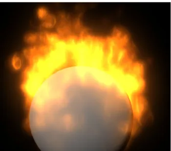
Maya dynamics can be used to create effects like steam, fire or rain. Fire-wise this method is best suitable for burning objects, objects leaving a trail or fireworks explosions. In the case of burning objects, the whole surface acts as an emitter. The motion of the flame itself isn’t as realistic as in the Fluid method, however this method provides much faster computing of simulation steps and rendering.

Figure 2.1: A burning sphere we created using Maya Dynamics method and rendered in mentalray.

2.1.2 Fluids method

This method can be used to create clouds, mist, fog, steam, smoke, fire, molten lava or ocean surface. In the scope of fire, this method is oriented mainly on creating realistic flame spread. It is best used to create fiery flamethrower-like projectiles, bonfires, explosions and nuclear blasts.

(15)

Contrast to Dynamics method, the fluid can spread only in a container, which must also contain the emitter. The motion of the fluid at each time step is simulated using solvers for the Navier-Stokes fluid dynamics equations. The extra data needed to define such fluid effect may slow the simulation exponentially, because more calculations are needed at every step. For this reason Maya provides non-dynamic fluid effects, in which the flame appear-ance is created using textures and the flame motion is achieved by keyframing texture attributes.

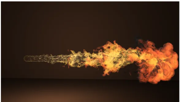
For another school project we created animation of a dragon destroying a city. Our result can be seen on figure 2.2. Base grid resolution is 150x150, emitting 500 particles per second. To better illustrate the complexity of such task - the simulation time was 22 minutes, rendering of one frame in 1920x1080 resolution using mental ray on hexa-core AMD Phenom II X6 1090T 3.2GHz was 82 minutes.

Figure 2.2: A flamethrower projectile we created in Maya using Fluid method and rendered in Mentalray renderer.

(16)

2.2 3D animation software plugins

The following list is a brief overview of some plug-ins aimed for fire modeling in 3D computer animation software. Most of them are compatible with at least one of the most used 3D animation software - Maya, 3Ds Max or Cinema4D.

2.2.1 AfterBurn

AfterBurn is an older plugin for creating volumetric effects. It’s usage lies mainly in the movie and video games industry of the 2000’s. It was used in motion pictures like Dracula 2000, Armageddon and Matrix Reloaded and video games like WarCraft 3 and StarCraft.

The method is based on building volumetric effects around the center of each particle. Each particle carries plethora of attributes (age, color, temper-ature, etc...), which can change over time of the animation using interpolation controllers. The usability and speed of the work flow are enhanced introduc-ing the Animation Flow Curves (AFC). This tool allows a clear plot-like overview of how different attributes of the particle change over time. This method also introduces wind fields (which they called Daemons) that can change the combustion direction so that the flame appears as progressing in one direction, swirling around a vortex or explosion in all directions. [d.o06]

(17)

2.2.2 FumeFx

FumeFx plugin can achieve one of the most realistic looking smoke and fire effects. On the top it also offers various improvements of workflow like GPU accelerated preview or multithreaded simulation. Developed by Sitnisati, this plugin is available for Maya and 3DsMax. This method was used for multiple award-winning feature films like The Avengers, Thor or Iron Man. [d.o13]

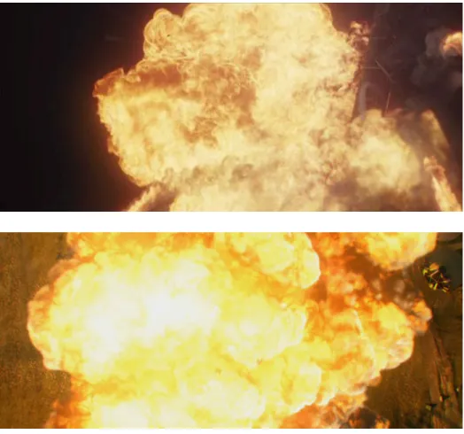
Figure 2.4: An example of flames created using FumeFx plugin. Pictures are from movies Ghost Rider and War Thunder, respectively.

(18)

2.2.3 TurbulenceFD

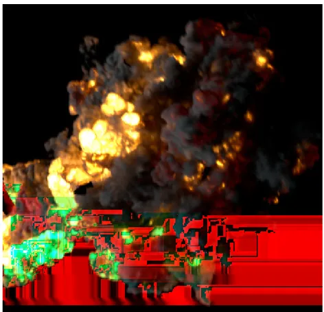
Developed by Jawset and available for Cinema4D and LightWave 3D (There is also a 2D version for Adobe After Effects). This system is based on solving the incompressible Navier Stokes equations. It utilizes a voxel grid to describe volumetric clouds of particles. The equations solutions describe the motion of fuid on the grid. Artist can paint sources of emission on any geometric object or particle system. In addition to fully tweakable fire shader the plugin provides a preset realistic fire shader based on the Black Body Radiation model. [Jaw09]

Figure 2.5: An example of a flame created using TurbulenceFD plugin. [Jaw09]

(19)

2.2.4 SOup upresNode

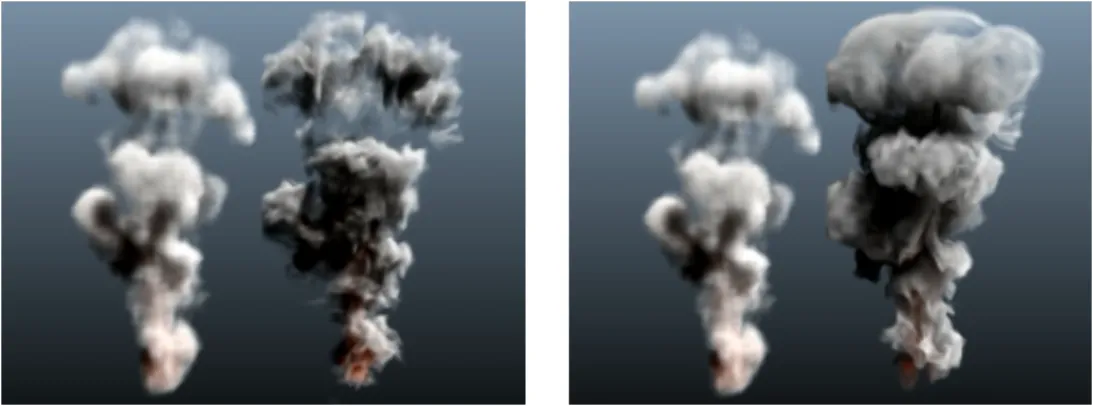
Animators often want to adjust the flame’s appearance in lower resolutions because it provides faster turnaround and after achieving desired behavior they want to increase the resolution to improve detail for the final rendering. SOup is a set of plugins that extend the procedural capabilities of Maya soft-ware. The upresNode plugin eliminates one major drawback of Maya’s fluids - that is, if you change the resolution of the grid the fluid behaves differently. Because of computational complexity, the tweaking of the flame’s appearance in high resolution can be very tedious. The plugin offers a new node that in-creases the resolution and local detail without changing the fluid’s behavior. It also allows additional detail at post processing by implementing wavelet turbulence algorithm proposed by [KTJG08]. [ea11]

Figure 2.6: An example of increasing the resolution of the grid using the SOup upresNode method utilizing Wavelet turbulence algorithm. [KTJG08]

2.2.5 PhoenixFD

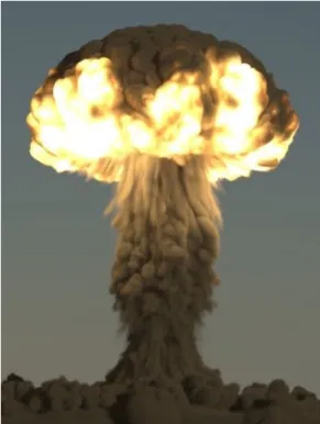
PhoenixFD is a plugin developed by ChaosGroup and available for 3DsMax and Maya. The plugin handles fire, smoke, explosions, liquids, foam and splashes. It offers a hybrid simulation system including grids and particles and is optimized to offer flexibility and speed even at very high particle

(20)

count. Fully utilizable with V-Ray renderer it offers proper refraction on liquids. [gro12]

Figure 2.7: Nuclear explosion created with PhoenixFD.

2.3 Shrek (2001)

This method was developed by DreamWorks and first appeared in the 3D animated movie Shrek (2001). The system’s main focus is on efficiency and complete control over visual appearance and behavior. The flame is based on parametric space curves that evolve over time according to multiple pro-cedural, hand-defined and physics-based wind fields. Physical properties are based on statistical measurements of natural diffusion flames. Around these splines is built an implicit surface with cylindrical profile. In this region the particles are point-sampled using volumetric falloff function. [LF02]

(21)

Figure 2.8: Screenshot from Shrek (2001). The flame was modeled using [LF02]. In this screenshot the flame evolves towards camera.

2.4 The Hobbit (2014)

The most complex animation simulation up to date was done by Weta Digital for the feature film Hobbit: The battle of the five armies. In this completely digital scene, a dragon destroys a wooden city situated on a lake. Combined simulations are used to achieve the resulting appearance, consisting of air, fire, water and rigid bodies simulations. Air flows and wind fields are modeled as volumes in which every piece of falling debris triggers wind movement, turbulence and pressure change. The dragon’s fiery breath consists of emitted particles which act in a fluid stream moving in a water-like simulation. This fluid then serves as a fuel for the fire itself, which creates viscous appearance of the fire and napalm-like spread in the environment. [MS13]

(22)

Figure 2.9: Screenshot from the destruction scene in The Hobbit: Battle of the Five Armies (2014)

(23)

Structural modeling of flames

3.1 Method overview

Here we provide an in-depth review of the state-of-the-art method for model-ing fire presented by [LF02] and used in the motion picture Shrek in the year 2001. This method constructs a flame animating system with emphasis not only on realism, but also on artistic appearance. It is based on particle sys-tem with appropriate and effective particle control. This syssys-tem provides a range of behavioral controls suitable for artistic animation. Realistic appear-ance is achieved using stochastic models of flickering and buoyant diffusion. Implementation of wind fields provides additional procedural control.Flame behavior includes moving sources, flickering, separation and merging, com-bustion spread and interaction with stationary objects.

Modeling flame movement as direct numerical simulation is very expen-sive computation-wise. These models often act in a 3D grid. As the grid res-olution increases, computational complexity raises by at least O(n3_{) [FM96]}

[SF95]. It is also difficult to implement intuitive control points for a physical based fire model. In addition, it is very hard for animators to achieve desired visual effect with numerical simulation, as even a small change in starting conditions can provide drastically different results.

The Structural modeling method provides different approach. It utilizes

(24)

the fact, that most of the visual aspects of the flame can be statistically mod-eled. By separating the statistic-based visual aspects of the flame, we are left with a set of structural elements which the animator can directly control by specified parameters. The statistical properties of the flame were measured on real flames. The model contains also numerous large-scale procedural controls such as wind, diffusion, fuel combustion or convection. These con-trols affect the local behavior of the flame particles. We will briefly cover the essential components of the model and then focus on the structure, particle creation and dynamics.

3.2 Essential components

This system utilizes different statistically-controlled or directly controlled elements. The whole model which can be divided into 8 components:

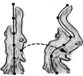
1. Central spine is formed using the central particles of the flame. The positions of these particles form a set of points which act as control points to an interpolating B-Spline curve. This curve defines the spine of the flame and is the main actor in the shape and behavior of the flame. As exact structure was not mentioned in [LF02], we in our pro-posed method decided to further divide the curve into smaller structure elements, which we will cover later in chapter 4. Although one curve is sufficient for defining one flame, multiple curves can act in a scene. When these curves collide with each other, the curve is not affected at all. However, when the curves are close to each other, the flames these curves define appear as if they were merging into one.

2. The splines evolve through space in time. Each point of the curve car-ries data of the flame’s height, age, temperature etc. The evolution depends on hand-defined, procedural and physics based wind fields. Some physical terms that affect the spline movement are based on sta-tistical measurements of real-life flames. The model also covers realistic adaptation of the flame to the movement of the source.

(25)

3. The curves can break when reaching specified lengths. The separation is based on the statistic measurements of natural diffusion flames. The separated segments act as individual splines, but they do not generate new segments. They convect freely in the environment affected by the wind field. The separated segments are given limited lifespan which can be also user-controlled. Along with the heuristic defining the breakaway height, the limitation of the separated spline lifespan and the rate of aging are based on engineering observations of real flames.

4. The region where actual particles of the flame are created is build using a cylindrical profile rotating around the central spline of the flame. The created particles gain the properties of the respective segments of the spline that spawned them. This region represents the visible part of the flame and provides a boundary with the oxidation region.

5. The first level of procedural noise is applied to particles created within the flame region. This noise is buoyant in nature, as it represents the combustion fluctuation of the flame base. It spreads up the flame profile based on the velocities of the structural elements. This noise is not based on any empirical observations, so Flow Noise is recommended, as it provided good visuals.

6. Transformation into parametric space of the structural curve is applied to the particles. Then a second level of noise is applied using a vector field created using a Kolmogorov frequency spectrum. This second level of noise simulates turbulent distortion details.

7. The particles are rendered with a volumetric or a fast painterly method. Thanks to the color adjustments of each particle based on the color properties of the neighboring particles, the flame elements can merge realistically.

8. We define procedural controls to account for position, intensity, lifes-pan, shape, color, size, evolution and behavior of the flames.

(26)

These 8 components form together a complex and general system for efficient and realistic flame animation along with some other similar natural fire effects. The computational complexity can be kept on a very low levels when desired, compared to numerical simulation approaches.

We do not cover the last 4 stages in detail because the main focus of this thesis is on the dynamics and structure of the flame.

3.3 Base Curve

Each central spline defining one flame is essentially a B-Spline curve with control points being the particles in the center of the flame. It is the funda-mental structure for the whole flame, as it affects the appearance and overall shape of the whole flame.

Figure 3.1: Spline movement impact on the shape of the whole flame. [LF02]

3.4 Dynamics

The particles in this model advance according to differential dynamics model describing a combination of physical terms as well as hand-defined procedural

(27)

wind fields. The differential equation is as follows:

∂xp

∂t =w(xp, t) +d(Tp) +Vp+c(Tp, t) (3.1)

where xp is the position of particlep, w(xp, t) is the displacement vector due

to wind fields, d(Tp) represents Brownian motion scaled by temperature of

the particle, Tp, the temperature of the particle p. Vp is the displacement

due to the motion of the source and c(Tp, t) is the motion due to thermal

buoyancy. The thermal buoyancy term is assumed to be constant over the lifespan of the particle, therefore

c(Tp, t) = −βtgy(T0−Tp)t2p (3.2)

whereβt is the coefficient of thermal expansion,gy is the vertical component

of gravity, T0 is the ambient temperature and tp is the age of the particle.

Because we are working with fire, the particle cannot get hotter than the environment, thus

∀p:T0 <=Tp

It depends on our cooling heuristic, but in general the t2

p term affects the

buoyancy term exponentially while (T0−Tp) decreases linearly, which results

in the rising of older particles despite their cold temperatures.

When a new particle is created at the source, it has initially the default user-specified parameters. If the source has velocity V, the particle is as-signed velocity -V. This negative velocity is completely sufficient to create realistic reaction of the flame to a moving source. You can see examples in figure 3.2.

3.5 Evolution of the flame

The flame moves according to combination of forces, some of which can be user-specified (like the procedural physics-based wind-fields) and some of them are statistical in nature and based on observation of natural diffusion

(28)

Figure 3.2: Torch waved through the air. A demonstration of flame adaptation to a moving source. [LF02]

flames. The motion is also influenced by hand-defined parameters (like am-bient temperature) and heuristics (cooling rate, aging rate). The evolution of the flame goes as follows:

1. In the first frame of the animation, a new particle p0 with initial

tem-perature T is created at the burning surface.

2. In the second frame of the animation, particlep0 is released into the

en-vironment, where it moves according to equation 3.1 using explicit Eu-ler integration method. [LF02] also mention that Runge-Kutta method for solving differential equations is sufficient and completely stable in this case.

(29)

3. A new particle p1 is generated at the surface and an interpolating

B-spline is created between particles p0 and p1. According to preset

den-sity n, n control points are uniformly sampled between them.

4. At the third frame a new particle p2 is created at the burning surface.

A new set of n control points is created between p2 and p1. All the

control points between p0 and p1 along with p0 and p1 themselves are

move according to equation 3.1. The interpolating B-Spline is then fitted to pass through all of the control points. The control points are then re-sampled so even distribution along the length of the spline is achieved. The first and last point of each segment is left unchanged, only the control points are re-sampled. This enables us to maintain constant detail along the whole flame.

5. For each additional frame of the animation we continue analogically with creating new segments. After reaching predefined height, the spline can separate.

3.6 Separation

In order to model flame separation as a statistical process, we must first divide the flame into regions according to the height of the flame. The first region will be the persistent flame region, it’s height denotedHp. In this region, the

flame will never separate and so the spline will be always continuous. Then the intermittent region, where we will decide if the flame will or will not separate. The height of the intermittent region is denoted Hi. And the final

region - the Buoyant plume - will be the part of the flame which is separated from the base of the flame. The plume will be short-lived and it will convect in the wind field freely.

The separation occurs in the intermittent section. When a particle ex-ceedsHi, we periodically test a random number against the probability

(30)

func-Figure 3.3: Illustration of persistent, intermittent and buoyant regions of the flame. [LF02] tion D(h) = √ 1 2π(Hi−Hp)/2 Z h −∞ e− h−|Vc| f /(2((Hi−Hp)/2)2) dh (3.3) wherehis the height of the flame at which we are testing,Hi is the height

of intermittent flame region, Hp is the height of persistent flame region,|Vc|

is the average velocity of the structural control points. f is the aproximate breakaway rate in Hz. According to the observations by [Dry01] f = (0.50±

0.04)(gy/2r)1/2 for circular sources with a radius r. We can also specify

D(h) ≡ 1 for h > Hmax, where Hmax is our desired maximal limit for the

flame height.

When we decide to separate the flame a portion of the spline is cutoff from the top of the flame. This portion ranges from the top to a randomly chosen point below. The distribution for this selection is not based on any observations. Normal distribution N(µ, σ2_{) proved sufficient with mean} _µ

(31)

and standard deviation σ chosen as:

µ=Hp + (Hi−Hp)/2 (3.4)

σ = (Hi−Hp)/4 (3.5)

The separated segment of the spline is not re-sampled back ton control points as this prevents additional local detail appearing in the separated segment. To account for lack of accurate way of fuel content determination, the particles in the spline are given a limited life-span of Ai3_{, where} _i _{is a}

uniform random variable in the range [0,1] and A is a length scale ranging from 1/24th _{of a second for small flames up to 2 seconds for a large pool fire.}

Because of i3 most of the breakaway flames have very short life-span.

3.7 Profiles

At this stage when the spline creation and evolution were covered, we can now focus on the visible part of the flame. The flame is defined as the region between the burning surface and an oxidizing agent. We utilize a volumetric model created by rotation of a 2D normalized profile around the axis of the Base spline. The profile can be hand-drawn or derived from photograph and creates a rotationally symmetric surface. In this 3D space fire particles are point-sampled and transformed into the spline structural curve. Two levels of procedural noise are added and then the particles are at their correct positions and are ready to be passed into the rendering stage.

(32)

Figure 3.4: Illustration of movement of the base splines and their impact on the overall look of the flame. [LF02]

(33)

Proposed method

We propose a method that creates the basic structure and dynamics for a controllable 3D fire effects. The flame’s motion is achieved by solving differ-ential equations that take account of procedural environmental factors as well as statistically measured factors, which are assessed on real-life observation and can be fine-tuned according to artistic taste.

Our method is based on DreamWork’s method Structural modeling of flames conceived by Arnauld Lamorlette and Nick Foster [LF02]. As the paper described this method in outlines and in general was short on details, we have created our own structure, chosen the wind fields implementation and heuristics. Parameters allowing greater control were added whenever reasonable.

4.1 Weighted dynamics model

We extend the Structural modeling dynamics differential equation to follow-ing form

∂xp

∂t =αw(xp, t) +βd(Tp) +γVp+δc(Tp, t) (4.1)

where α, β, γ andδ are weights corresponding respectively to the wind field, diffusion, source motion and buoyancy terms. Setting the weights constant or interpolating their values over time of the animation creates additional

(34)

controls that help us shape the behavior of the flame to our needs.

Figure 4.1: Example of modifying the parameters of equation 4.1. In the left δ= 1, in the right δ = 0.1. This scene has uniform wind

field which blows to the right.

4.2 Amortization

The [LF02] paper was not describing any heuristic for the amortization of particle attributes. We have decided to use linear techniques of temperature decay

Tt+1 =max(Tt−c∆t, T0) (4.2)

where Tt+1 is the temperature of the particle in the next time step, Tt is the

temperature in current time step, c is the cooling rate parameter and ∆t

is the size of one time step. T0 is the ambient temperature. Since we are

modeling fire, we have decided that the particle temperature can not drop below ambient temperature.

Similarly we defined the age amortization as

(35)

wherett+1is the age of the particle in the next time step,ttis the temperature

in current time step, a is the parameter specifying aging rate and ∆t is the length of one time step. We also define maximal age tmax. If age of the

particle reaches tmax, the particle dies.

The values for parameters c and a are chosen to suit our needs and are used as one of the controls for flame behavior and appearance. They mainly affect rendering, particle color and buoyancy in the upper stages of the flame.

4.3 Structural elements

As the method described the structure very loosely, we created our own structures, their hierarchy and attributes. The center spline forming the spine of the flame still plays major role in the flame appearance and has the greatest impact on visuals and dynamics.

4.3.1 Emitter

The flame creation is handled by an emitter. It is the most fundamental element as it carries important parameters required for creation of the Base splines of the flames. The scene can contain multiple emitters and each emitter can emit multiple Base splines, which each form an individual flame. Due to the chosen rendering methods, all the flames emitted from one emitter appear as if they joined together to form one flame. So while it may look like each emitter emits only one flame, in fact they are emitting multiple flames which quickly visually merge. Each emitter has its position, velocity, density and radius of the burning source surface.

(36)

Table 4.1: Table of emitter attributes Attribute

name

Notation Description

Origin o Specifies the position of the emitter Veclocity ~v Velocity of the emitter

Density n Number of Base splines the emitter emits Radius r Radius of the burning surface

4.3.2 Base spline

The Base spline is emitted from emitter and consists of spline segments. At every frame, new segment is created at the bottom of the spline and according to random distribution presented in section 3.6. One or more segments can partly separate and form a new spline. The length Lof the base spline s is

L=

n−1

X

i=0

lsi (4.4)

where n is the number of segments of the spline and lsi is the length of i-th

segment in the spline.

Figure 4.2: Our visualization of Base spline element. Red points are end points separating the segments, black points are control points and the

spline is interpolating Catmull-Rom spline.

4.3.3 Base Spline segments

Each spline forms a spine for one individual flame. The individual splines consist of s segments. Each segment consists of a start point ps, end point

(37)

pe and n control points cp0. . .cpn−1. The density of the control points

spec-ified by n doesn’t need to be uniform in all segments of spline, as when we introduce flame separation, the spline can break in the middle of a segment, forming 2 splines with non-uniform density. The number of control points in the newly created segments can be user-specified to achieve desired balance between computational complexity and detail level. The segments act as in a linked list, with the last point of i−1 -th segment being the start point of i-th segment, pei−1 =psi. At i-th segment a B-Spline is interpolated from

psi through all control points of that segment arriving atpei. Thus a spline

segment with density nconsists of n+ 2 particles (start point, end point and

n control points) and containsn+ 1 segments.

The length of a spline segment is defined as the length of the spline starting in ps, passing through every control point and ending in pe. See

equation 4.7

4.3.4 NURB as a Spline segment

It is not exactly stated in [LF02] what properties should the B-Spline curve have. The first version of our implementation contained a Non-uniform Ra-tional B-Spline as it offered controls superior to general B-Spline. We used the general form of NURBs curve

C(u) = Pk i=1Ni,nwipi Pk i=1Ni,nwi (4.5) wherek is the number of control pointsp,wi are their corresponding weights

and Ni,n are the recursively-defined basis functions of a NURB spline.

The intention was to control the visuals through the knot vectors, weighted control points and degree of the NURBs. However in the later phases where re-sampling of the control point in each frame is required (see 4.4), the NURB under-performed due to its lack of ability to pass through all the control points and the whole spline tended to flatten more and more during the simulation.

(38)

In the end we’ve decided to utilize Catmull-Rom spline, as it proved sufficient results while allowing us to pass through each control point.

4.3.5 Catmull-Rom spline as Spline segment

We define the Catmull-Rom spline as

p(t) = 1, t, t2, t3        0 1 0 0 −τ 0 τ 0 2τ τ −3 3−2τ −τ −τ 2−τ τ−2 τ               pi−2 pi−1 pi pi+1        (4.6)

where t is the interpolation parameter, τ is the tension and pi−2. . . pi+1

are points defining the spline. The spline itself is drawn only between points

pi−1 and pi, pointspi−2 pi+1 serve only for computing the required tangents.

Note that p(0) =pi−1 and p(1) =pi.

This spline proved sufficient for our implementation and provided satis-fying results. We define the length of the spline as

L= n−2 X t=0 p t n−1 −p t+ 1 n−1 (4.7) where n is our chosen sampling. In our work we found n= 100 sufficient.

Figure 4.3: Example of different tension values for the Catmull-Rom spline. On the left τ = 0.5, on the rightτ = 2.

(39)

4.4 Evolution of the flame

In this section we present detailed description of the modified evolution of flame in detail:

1. We can have one or multiple flame emitters. Each emitter has it’s position p, radius r, velocity v and b, which is the number of Base splines it will produce concurrently. Following steps are the same for each emitter in the scene.

2. In the first time step of the animation, the emitter creates a new seg-ment. This segment is created at the present position of the emitter and consists only of one particle p0 which will gain the user-specified

values of initial temperatureTp0 and initial agetp0 (typically zero). The

particle also inherits the position pand the velocity−v of the emitter. Gaining the negative velocity of the emitter covers the realistic flame behavior when the burning surface containing the emitter moves. This particle acts as the start point and the end point of the segment, while the segment does not have yet any control points and thus no B-Spline. 3. In the second time step frame of the animation, particle p0 is released

into the environment, where it moves according to 4.1 and is amortized with the methods proposed in 4.2. New particle p1 is generated at

the origin of the emitter and N control points are uniformly sampled between the particles p0 and p1. The control points have their age and

temperature linearly interpolated between the values of the points p0

and p1. We have tried also assigning the properties of p0 to all of the

control points, but this provided noticeable visual separation of the segments. All the particles of the segment then move and amortize analogically. Every following segment is created and moved in the scene analogically. The separation and flickering occurs as in described in section 3.6.

(40)

We create a normalized 3D profile by symmetrical rotation of the 2D profile. We then randomly generate s particle positions and test them against the profile using rejection sampling. The resulting set of parti-cles is then mapped from the parametric profile space into the space of the deformed Base spline using cylindrical coordinates. The particles inherit the age and temperature attributes from the structural elements on the corresponding level of the spline.

4.5 Wind Fields

We model our wind fields based on the method proposed by [WH91]. We define 4 types of wind-fields - Uniform, Sink, Source and Vortex. Sink, Source and Vortex wind fields are circular and have always one fixed axis. Each acting wind field displaces the position of particle xp. The displacement

vector is affected by time step of our simulation, so it is scaled by ∆t.

Figure 4.4: Schematic describing the sink, vortex, uniform and source types of the wind fields.

For the Uniform wind-field it is sufficient to specify only the direction and strength. However for the circular types this is not sufficient, so we specify the displacement vectors in cylindrical coordinates (r, θ, z). For the Source wind-field placed at the origin the displacement vector is defined as

vr =

s

(41)

wheres is the strength of the wind field and r is the r coordinate of our particle’s position in cylindrical coordinates and ∆t is size of our chosen time step. The Sink wind-field produces the same displacement vector as Source wind-field, except the stength parameter s is set negative.

As the Vortex wind-field rotates the given point around the wind-field’s origin, it changes only the angle θ in cylindrical representation. The dis-placement vector for Vortex wind-field placed at origin with strength s is then given by

vr = 0; vθ =

s

2πr∆t; vz = 0; (4.9)

wheres is the strength of the wind field and r is the r coordinate of our particle’s position in cylindrical coordinates and ∆t is size of our chosen time step.

The resulting displacement vectorw(xp, t) of equation 4.1 is the sum over

each wind-field in the system.

w(xp, t) = n

X

i=0

vi =vvort(xp, t) +vsink(xp, t) +vsource(xp, t) +· · · (4.10)

4.6 Separation and Flickering

The separation stage of the flame is modeled as presented in section 3.6. We approximate the integral in the probability function in equation 3.3 using following method Z h −∞ e− h−|Vc|_f /₍2((Hi−Hp)/2)2) dh= h−g N h X i=g e− i−|Vc|_f /₍2((Hi−Hp)/2)2) (4.11) where g is the chosen lower point from which we start approximating the integral andN is the number of steps that we wish to sample betweeng and

h. Satisfying results were obtained using h=−100 and N ≈107_.

To select the height of the transformation, we model the Gaussian distri-bution as Box-M¨uller Transformation. Given variables x1 and x2 which are

(42)

Figure 4.5: Example of flame behavior in combination of Vortex and Source wind-fields.

uniformly and independently distributed between 0 and 1, we define z1 and

z2 as z1 = p −2 lnx1cos(2πx2) (4.12) z2 = p −2 lnx1sin(2πx2) (4.13)

giving z1 and z2 normal distribution with mean µ= 0 and variance σ2 = 1.

Due to our structure, after selecting the proper height of separation, we need to find the corresponding point on the spline.

(43)

Figure 4.6: Example of spline separation. Evolution of the same spline with the same settings and wind fields. In the left, the separation is disabled, in

the right it is enabled.

4.7 Flame profile generation

After specifying the 2D normalized flame profile, we create a normalized 3D cube where we rotate the 2D profile around the Y axis and thus achieve a symmetric space in which we can create particles. The particles’ positions are randomly selected using uniform distribution and then tested against the symmetric 3D profile whether they are accepted or rejected. The number of accepted samples depends on the shape of the specified 2D profile. For most of the used profiles, around one half of the samples were rejected.

4.8 Visualization of the particles

As the rendering part of the [LF02] technique was quite complex and out of the scope of this thesis, we have decided to implement simplified particle rendering using billboards. We are rendering each particle as a rectangle

(44)

Figure 4.7: Examples of different profiles and their effect on the shape of the flame. The amortization shader is turned off.

which always faces the camera and is painted with miniature flame particle texture.

Since we have all the attributes of the painted particle at our disposal, we modify the color of each particle according to its age and temperature. The temperature of the particle is affecting red, green and blue channels of the particle color, while age determines the value of alpha channel responsible for particle transparency. The amount of darkening of the particle is based on the color of the texture, but for most textures that we tried we found suitable this method:

cp =cp

Tp Ti

4 −T0

where cp is the color of particle p,Tp is the temperature of the particlep, Ti

is the initial temperature which is each particle assigned at the moment of creation at the base of each emitter and T0 is the ambient temperature.

Next we change the transparency of the particle. We use

ap = 1−

tp

tmax

(45)

the maximal age at which particles die.

(46)

Chapter 5 Implementation

Our method is implemented in C# and developed on operation system Win-dows 10 Technical Preview. The compiler is .NET 4.5. IDE used is Microsoft Visual Studio 2013 Ultimate. GUI is implemented using WinForms, the vi-sualization using OpenGL API v3.3. To access OpenGL in C#, we use OpenTK library, v1.1.

The data structure can be divided into 3 main parts:

• Flame representation (Emitters, Splines, Particles)

• Parametric controls (Wind-Fields, Settings, Differential equation solver)

• Helper classes (Camera, Settings, GUI elements, Converters, Math classes)

5.1 Flame representation

Understanding of the flame structure is essential to understand the algo-rithms and dynamics described later in this chapter. This section covers the classes that build up the whole flame structure including the particles.

(47)

Figure 5.1: Class diagram depicting representation of the flame in our structure.

5.1.1 Spline structure

Because the structure is not trivial, we present a bottom-to-top explanation of the whole structure responsible for representation of one burning surface. We start with describing the basic particle types and move up the structure until we reach the topmost class.

(48)

Smallest elements

The essential structures are Spline particles, which carry information about the age, temperature, position and velocity of the particle. TheSplineP article

is an abstract class, we define the different particle types using inehritance. We have three types of particles: F ireP article for representing the visi-ble part of the flame, ControlP oint for representing the control points of eachSplineSegment andSplineEndP ointfor representing the first and last point of each SplineSegment. They all all inherit the basic attributes from

SplineP article class.

TheCatmullRomSplineSegmentalso belongs into the scope of the small-est elements of our structure. It represents one segment of a Catmull-Rom in-terpolating spline. Despite being defined by four spline particlespi−2. . . pi+1,

it represents only the part between particles pi−1 and pi. It contains basic

methods of finding the corresponding point on the spline by implementing equation 4.6 For details, see section 4.3.5.

Spline Segment

The SplineSegment class contains two SplineEndP oints representing the first and last particles, a linked list of n ControlP oint particles and a Cat-mullRomSpline class, which covers the representation of the spline stretching from the first SplineEndP oint through all theControlP oints in the linked list to the last SplineEndP oint. Each segment of this spline is represented by CatmullRomSplineSegment class.

Spline segment contains functionality responsible for evolution and amor-tization of its particles as well as methods for computing the length of the spline or finding a particle at specified height. CatmullRomSpline class is responsible for re-sampling of the control points.

(49)

Base spline

The BaseSpline class consists of linked list of SplineSegments. It is used for representing the persistent flame part as well as the separated buoyant plumes. While the persistent Base Splines have fixed life time specified by parametertmax, the separated segments are given limited life-span. This class

is also responsible for drawing itself in the visualization window, so methods and data structures required to draw points and polylines in OpenGL are implemented.

Its functionality covers the calculation of the average velocity of all control points of the spline, the separation of the spline and also a method for finding particle at specified height.

Spline Emitter

The topmost class in our structure is the SplineEmitter. It has specified radiusr, positionpand a spline counts. It also has two linked list structures, one representing persistent Base Splines and one representing the separated Base Splines. In the specified interval it emits s new Base Splines. It also governs functionality responsible for testing whether to separate the spline and it hosts theP articleM anager class responsible for managing the visible part of the flame.

Particle manager

The P articleM anager class is responsible for building up the visible part of the flame by creating the particles represented byFlameParticle class. Every spline emitter has one instance of ParticleManager. By utilizing the flame profile represented as an array of floating point numbers, it governs the cre-ation of the particles for all the splines of the corresponding SplineEmitter. By using the helper classes that implement the needed transformations be-tween normalized 3D profile space and structural spline space it outputs the flame particles with correct attributes and positions. Since it is responsible

(50)

also for the rendering of the particles, this class also covers methods and data structures necessary to setup OpenGL shaders and buffer objects.

5.2 Parametric controls

In this section we will cover data structures responsible for the dynamics and control of the fire. We can control the fire by specifying various values for parameters describing the dynamics model as well as by specifying multiple wind-field types in the scene.

5.2.1 Settings and parameters

In our application the setting of the constants and parameters are imple-mented as a singleton classes having private static fields representing each parameter. Each field is encapsulated with non-static C# getter and setter to allow binding to controls in the main form.

Following is a table of the parameters we can change through the user interface to change the behavior of the flame. This is only a digest of the flame-controlling parameters, as these classes contain more parameters which are not related to the flame.

Table 5.1: Fire-controlling attributes in class MainMovementEquation Notation Type Description

α f loat Wind-Field term weight

β f loat Diffusion term weight

γ f loat Source velocity term weight

δ f loat Buoyancy term weight

βt f loat Thermal expansion coeficient

T0 f loat Ambient temperature

(51)

Table 5.2: Fire-controlling attributes in class SplineSettings Notation Type Description

shalpha bool Activated transparency in amortization shader

shdark bool Activated darkening in amortization shader

speed int Simulation speed in ms

growth int Simulation steps needed to create a new seg-ment

Ssampling int Catmull Rom sampling density

fire density

int Number of Fire Particles per segment tested in rejection sampling

start age f loat Initial age of newly created particles

A f loat Life time of separated segments.

τ f loat Tension of the Catmull-Rom splines.

starttemp f loat Temperature of newly created particles

cooling f loat Temperature amortization per one time step

aging f loat Life amortization per one time step

agemax f loat Maximal life-time of particles

CPcount int Number of control points per one

SplineSeg-ment

Hp f loat Height of the persistent flame stage

Hi f loat Height of the intermittent flame stage

Hmax f loat Height after which the flame always separates

5.2.2 Wind-fields

As in particle implementation, in wind-fields inheritance plays major role and is essential to the structure. We define one abstract class wind-field which has key method shared across all types of wind-fields -getDisplacement. This method returns the displacement vector affecting given position. The uniform

(52)

wind field has only direction and strength attributes. The circular wind-fields also utilize inheritance, because they all share the same attributes - origin and strength. The difference is in the getDisplacement function, which each representation overrides.

Figure 5.2: Class diagram depicting representation of the wind in our structure.

5.2.3 Simulation step calculation

SplineCalculator is a singleton class responsible for calculation of the main differential equation in each time step. It also contains a reference to a list containing all the wind-fields defined in a scene. After taking a SplinePar-ticle descendant with required parameters such as temperature and age, it returns the displacement vector calculated by taking into account all four main equation terms - wind fields, diffusion, source movement and buoyancy, as well as their corresponding weights.

(53)

5.3 Key algorithms

Here we present some key algorithms we implemented that were essential to our proposed method. Because of limited size of this thesis we could not mention all the interesting methods, so we have selected the most important ones. You can review the rest in the source code, which is attached to this thesis.

5.3.1 Control points re-sampling

In each time step we need to re-sample the control point positions according to a Catmull-Rom spline associated with the given segment. This algorithm takes place in theCatmullRomSpline class, which represents the spline of one SplineSegment. If theSplineSegment has n control points, the corresponding CatmullRomSpline contains a linked list ofn+ 1CatmullRomSplineSegment instances.

Algorithm 5.1 Re-Sampling of the control points

spline = new CatmullRomSpline(SplineEndPoints, ControlPoints) newSegmentLength = spline.Length/CatmullRomSplineSegments.Count height = 0

for i=0 to CatmullRomSplineSegments.Count-2 do height += currentSegment.Length

newPosition = spline.getPointAtHeight(height) newControlPointPositions.Add(newPosition) end for

return return newControlPointPoisitions

5.3.2 Box-M¨

uller transformation

We use Box-M¨uller transformation principle in determining the separation height of the spline. Using two uniformly distributed random variables we can return a random variable with given mean and standard deviation.

(54)

Algorithm 5.2 Box-M¨uller transformation Input: mean, standardDeviation

r1 = uniform random in range [0,1]

r2 = uniform random in range [0,1]

randNormal =√−2 logr1sin 2πr2

return mean+standardDeviation*randNormal

5.3.3 Wind-Fields transformation

Each wind-field affects the position of the particle in cylindrical coordinates. Here we present general algorithm depicting the necessary transformations for circular wind-fields.

Algorithm 5.3 Wind-Fields transformation Input: position

positionInWFcoords = position - windfield.origin

cylindricalPos = CartesianToCylindrical(positionInWFcoords) cylindricalDisplacement = ∆t wf.getDisplacementVector newCylindricalPos = cylindricalPos + cylindricalDisplacement

newCartesianInWFPos = CylindricalToCartesian(newCylindricalPos) return (newCartesianInWFPos+origin) - position

5.3.4 Simulation step calculation

This algorithm takes place in SplineCalculator class. The input parameter is a SplineParticle instance. The method returns new velocity for the given particle.

5.3.5 Integration approximation

Here we cover our approximation of the integration needed in testing whether to separate spline at a given height. In the final release this method was

(55)

re-Algorithm 5.4 Simulation step calculation Input: particle

displacement = (0,0,0)

for all windfield in windFields do

displacement += α windfield.getDisplacement(particle.position) end for

displacement += β normalizedRandomVector*particle.Temperature displacement += γ particle.SourceVelocity

displacement += δ−βtgy(T0−particle.temperature) particle.age2∆t

return displacement

placed with double exponential transformation from MathNet library because it provided better calculation times.

The following algorithm takes min and max as input parameters spec-ifying the range at which we want to calculate the integration. stepsize is are also among input parameters. Step size is directly proportional to com-putation error and inversely proportional to time complexity. func(x) is the desired function we wish to integrate.

Algorithm 5.5 Integration approximation Input: min; max; stepSize, funct(x)

result = 0

for step = min; min <max; step+= stepSize do result += funct(step) * timeStep;

end for return result

5.3.6 Spline space mapping

The 5.6 algorithm is used in each time step to map theFireParticle instances into the space of the structural spline curve. It also sets the correct values for the particles age and temperature based on their height on the spline. The

(56)

input parameters are position of the particle in normalized 3D space profile and spline to which we wish to map the position.

Algorithm 5.6 Spline space mapping Input: position, spline

cylindrical = CartesianToCylindrical(position)

particle = spline.getParticleAtHeight(cylindrical.Z*spline.Length) nextStep = min(cylindrical.Z+0.001, 1)

particle2 = spline.getParticleAtHeight(nextStep*spline.Length) newZVector = normalize(particle2.position - particle.position) unitX = (1,0,0)

unitY = (0,1,0)

helpingVector = (newZVector == UnitX) ? UnitY : UnitX

newXVector = normalize(cross(newZVector, newZVector+helpingVector)) radialDisplacement = (newXVector*spline.radius)*cylindrical.r

radialDisplacement = radialDisplacement * CreateRotationMatrixFro-mAxisAngle(newZVector, cylindrical.θ)

particle.position += radialDisplacement; return particle

5.4 GUI

We provide user interface covering a wide range of controls. The controls are logically divided based into 5 panels arranged as tabs in a TabControl instance. Thanks to implementing the settings classes as singletons with public encapsulated fields we can directly bind the specified fields to their GUI elements. The logical values are represented via checkboxes, numerical parameters are utilizing numericUpDown controls.

The GUI also contains controls allowing adding and removing wind fields and emitters.

(57)

Figure 5.3: Example of GUI elements for controlling the dynamics and separation of the flame.

(58)

Chapter 6 Results

The implemented method was tested on a notebook with Intel Core i3 350m processor 2.26Ghz (2 cores), 4Gb of RAM and an ATI Radeon 5145 graphics card with 512Mb of memory. The simulation ran above 30 frames per second with one emitter containing one spline. The spline contained up to 15 spline segments active and testing 100 particles per segment. Increased particle or segment count led to a rapid drop in frames per second. The method proved controllable and usable up to 100 000 particles per segment, although when populating the scene with this many particles, the application FPS count started to incline towards fps of applications using complex numerical solutions and offline rendering methods.

6.1 Direct control methods

One of the main goals of this work was to provide wide range of controls over the flame behavior and appearance. In professional applications the fire simulations are controlled via multitude of parameters and even slight change can produce drastically different results. Our application shares this feature. In this section we provide a few examples of achieving different goals with our simulation. Some of these results can be achieved by different settings, each of which produces different side-effects. This feature is also present in

(59)

professional methods.

6.1.1 Dominating the movement with wind-fields

Should we want to boost the effect of wind-fields, we simply increase the wind-field weight α in the main differential equation. If we would like to boost only one specific wind-field, we increase its strength parameter. In our application we found that in order to see this effect in a bigger scope, often prolonging the spline is needed. For examples on this topic, see section 6.1.3. As the buoyancy term is exponentially proportional to the flame age, it easily overpowers the wind-fields effect in the main equation. If we want to model loops of fire or bend the flame towards one point using wind-fields, we need to suppress the buoyancy term. Values in the range [0, 0.1] for buoyancy term δ proved usable.

6.1.2 Smoke simulation

Due to amortization shader, the colder the particles are, the darker texture they render in our billboarding visualization. If we want to boost the dark-ening the tip of the flame, we need to ensure that these particles are colder. Since the amortization shader takes account of the temperature span of the particles, reducing the initial temperature is not the right way to do this. We can achieve this effect by increasing the cooling rate. The side effects of this cooling are that the flame temperature can more quickly drop to the levels of ambient temperature, at which the buoyancy term of the main equation entirely loses its effect.

6.1.3 Prolonging the spline

Most common requirement for the flame behavior would be to prolong it’s length. In order to achieve this, the user must first understand when are the end segments of the flame destroyed. Basically, the main precursor for de-stroying the end segments is their current age affected by life-span parameters

(60)

Figure 6.1: Direct control using wind-fields. In the first image we see uniform wind field colliding with source wind-field. The second image is

combination of uniform and vortex wind-fields. Both examples have diffusion and buoyant terms suppressed to ≈ 0.1

- initial age and aging rate. With flame separation disabled, increasing the initial age and decreasing the aging rate is sufficient to increase the length of the flame. However the separation is often needed and it complicates achieving what might at first seem like a simple task. While the sufficient life-span is required, the length of the spline comes into play. As the sep-arated segments maximum life-span gets modified and scaled by a cubed uniform random variable in the range [0,1], once the separation occurs, the flames are short-lived and thus the flame appears shorter. One way of fixing

(61)

Figure 6.2: Example of darkening by increased cooling. The first image has cooling set to -0.5, the second has cooling -2.0

this issue is changing the lengths describing the persistent and intermittent height, as well as specifying the maximum length at which the separation oc-curs with 100% probability. The other way is increasing the apparent length of the flame by suppressing the diffusion factor. This effectively flattens the Catmull-Rom spline in between the segment end points, thus providing a shorter segment and in turn increasing the amount of segments which fall under the persistent and intermittent flame regions.

6.1.4 Artifacts

With many parameters and many ways to control our model, many ways to break the model emerge. While we tried to restrict the inputs for the parameters in a safe manner, the number of different parameter combinations allow for unpredicted behavior. One particularly interesting effect comes with

(62)

Figure 6.3: Example of flattening the spline by reducing the diffusion term

β. The left image has β = 1, in the secondβ = 0.1

(63)

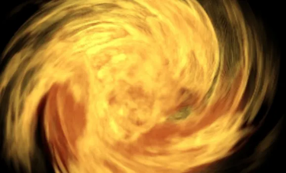
displaced around the whole scene, making the Catmull-Rom spline stretch to great lengths and create random shapes. While by restricting the spline length we can produce a chaotic fireball effect, prolonging the spline with uniform profile provides a tentacles-from-hell like appearance.

Figure 6.4: The tentacles of hell achieved by setting Catmull-Rom tension

τ = 2 and setting the particles tested against each segment to 100 000. During this simulation the FPS was essentially zero

(64)

Chapter 7 Conclusion

In this thesis we have presented a method for modeling dynamics of fire. We have presented an improvement of the structural modeling method and implemented usable application with a wide range of user controls for al-tering the behavior and visualization of the flame. The desired effect can be achieved by multiple paths and different configurations, which can pro-duce different side-effects. This principle is present across all state-of-the-art flame modeling software. Because of this complexity, complete control over the flame requires at least a shallow understanding of dynamics principles presented in this thesis.

In the future work we need to enhance the generation of fire particles with noise and displacement to produce more realistic flame profiles. Wind fields could be enhanced to allow for more complex wind flows changing over time. Collision with objects in the scene needs to be added. Export to external rendering software such as Maya could prove beneficial. More complex visualization and high-quality offline rendering would also be useful. There is always space for optimization and parallelization.

(65)

[Aut14] Autodesk. Maya 2015 user guide. http://help.autodesk.com/

view/MAYAUL/2015/ENU/, 2014. [Online; accessed 21-April-2015].

[d.o06] Sitni Sati d.o.o. AfterBurn plugin. https://www.afterworks.

com/AfterBurn.asp?ID=2, 2006. [Online; accessed

21-April-2015].

[d.o13] Sitni Sati d.o.o. FumeFx plugin.https://www.afterworks.com/

FumeFX_Maya/Overview.asp?ID=1, 2013. [Online; accessed

21-April-2015].

[Dry01] Dougal Drysdale. Intro to Fire Dynamics. Wiley, 2 2001.

[ea11] Peter Shipkov et al. SOup plugin. http://www.soup-dev.com/

examples2_1.htm, 2011. [Online; accessed 21-April-2015].

[FM96] Nick Foster and Dimitri Metaxas. Realistic animation of liquids. Graph. Models Image Process., 58(5):471–483, September 1996.

[gro12] Chaos group. PhoenixFD plugin. http://www.chaosgroup.

com/en/2/phoenix_maya.html, 2012. [Online; accessed

21-April-2015].

[Jaw09] Jawset. TurbulenceFD plugin.https://www.jawset.com/, 2009. [Online; accessed 21-April-2015].

[KTJG08] Theodore Kim, Nils Th¨urey, Doug James, and Markus Gross. Wavelet turbulence for fluid simulation. In ACM SIGGRAPH

(66)

2008 Papers, SIGGRAPH ’08, pages 50:1–50:6, New York, NY, USA, 2008. ACM.

[LF02] Arnauld Lamorlette and Nick Foster. Structural modeling of flames for a production environment. In Proceedings of the 29th Annual Conference on Computer Graphics and Interactive Tech-niques, SIGGRAPH ’02, pages 729–735, New York, NY, USA, 2002. ACM.

[MS13] Jason Diamond Mike Seymour, Matt Walin. The VFX show. http://www.fxguide.com/thevfxshow/

the-vfx-show-177-the-hobbit-the-desolation-of-smaug/,

2013. [Online; accessed 21-April-2015].

[SF95] Jos Stam and Eugene Fiume. Depicting fire and other gaseous phenomena using diffusion processes. In Proceedings of the 22Nd Annual Conference on Computer Graphics and Interactive Tech-niques, SIGGRAPH ’95, pages 129–136, New York, NY, USA, 1995. ACM.

[WH91] Jakub Wejchert and David Haumann. Animation aerodynam-ics. In Proceedings of the 18th Annual Conference on Computer Graphics and Interactive Techniques, SIGGRAPH ’91, pages 19– 22, New York, NY, USA, 1991. ACM.

(67)

2.1 A burning sphere we created using Maya Dynamics method and rendered in mentalray. . . 4 2.2 A flamethrower projectile we created in Maya using Fluid

method and rendered in Mentalray renderer. . . 5 2.3 Example of vortex daemon wind field in AfterBurn. . . 6 2.4 An example of flames created using FumeFx plugin. Pictures

are from movies Ghost Rider and War Thunder, respectively. . 7 2.5 An example of a flame created using TurbulenceFD plugin.

[Jaw09] . . . 8 2.6 An example of increasing the resolution of the grid using the

SOup upresNode method utilizing Wavelet turbulence algo-rithm. [KTJG08] . . . 9 2.7 Nuclear explosion created with PhoenixFD. . . 10 2.8 Screenshot from Shrek (2001). The flame was modeled using

[LF02]. In this screenshot the flame evolves towards camera. . 11 2.9 Screenshot from the destruction scene in The Hobbit: Battle

of the Five Armies (2014) . . . 12 3.1 Spline movement impact on the shape of the whole flame. [LF02] 16 3.2 Torch waved through the air. A demonstration of flame

adap-tation to a moving source. [LF02] . . . 18 3.3 Illustration of persistent, intermittent and buoyant regions of

the flame. [LF02] . . . 20

(68)

3.4 Illustration of movement of the base splines and their impact on the overall look of the flame. [LF02] . . . 22 4.1 Example of modifying the parameters of equation . . . 24 4.2 Our visualization of Base spline element. Red points are end

points separating the segments, black points are control points and the spline is interpolating Catmull-Rom spline. . . 26 4.3 Example of different tension values for the Catmull-Rom spline.

On the left τ = 0.5, on the right τ = 2. . . 28 4.4 Schematic describing the sink, vortex, uniform and source

types of the wind fields. . . 30 4.5 Example of flame behavior in combination of Vortex and Source

wind-fields. . . 32 4.6 Example of spline separation. Evolution of the same spline

with the same settings and wind fields. In the left, the sepa-ration is disabled, in the right it is enabled. . . 33 4.7 Examples of different profiles and their effect on the shape of

the flame. The amortization shader is turned off. . . 34 4.8 The effect of amortization shader. . . 35 5.1 Class diagram depicting representation of the flame in our

structure. . . 37 5.2 Class diagram depicting representation of the wind in our

structure. . . 42 5.3 Example of GUI elements for controlling the dynamics and

separation of the flame. . . 47 6.1 Direct control using wind-fields. In the first image we see

uniform wind field colliding with source wind-field. The second image is combination of uniform and vortex wind-fields. Both examples have diffusion and buoyant terms suppressed to ≈0.1 50 6.2 Example of darkening by increased cooling. The first image

(69)

6.3 Example of flattening the spline by reducing the diffusion term

β. The left image hasβ = 1, in the second β = 0.1 . . . 52 6.4 The tentacles of hell achieved by setting Catmull-Rom tension

τ = 2 and setting the particles tested against each segment to 100 000. During this simulation the FPS was essentially zero . 53

DRAGON FIRE MODELING AND SIMULATION IN 3D FOR COMPUTER ANIMATION Diploma thesis