The Review of International Organizations (2020) 15:29–73
How to evaluate the effects of IMF conditionality
An extension of quantitative approaches and an empirical
application to public education spending
Thomas Stubbs1,2 &Bernhard Reinsberg2,3&Alexander Kentikelenis4& Lawrence King5
#The Author(s) 2018 Abstract
Following calls for a more disaggregated approach to studying the consequences of IMF programs, scholars have developed new datasets of IMF-mandated policy reforms, or
‘conditionality.’Initial studies have explored how conditions have, inter alia, affected tax revenues, public sector wages, and health systems. Notwithstanding the important con-tributions of these studies, a methodological quandary arises as to how to quantitatively examine the effects of conditionality, as distinct from other aspects of IMF operations (e.g., credit, technical support, or aid and investment catalysis). In this article, we review and advance these methodological debates by developing an identification strategy for addressing the multiple endogenous components of IMF programs. We begin by survey-ing the main strategies for studysurvey-ing the effects of IMF programs: matchsurvey-ing methods, instrumental variable approaches, system GMM estimation, and variants of Heckman estimators. We then adapt these methods for studying the effects of conditionality per se. Specifically, we utilize a compound instrumental variable design over a system of three equations to address sources of endogeneity related to, first, the IMF participation decision and, second, the conditions included within the program. In Monte Carlo simulations, we demonstrate that our approach is unbiased and performs better than alternatives on standard diagnostics across a range of scenarios. Finally, we apply these methods to investigate how IMF programs impact government education spending as a share of GDP on a sample of 132 developing countries for the period 1990 to 2014, finding exposure to an additional condition results in a 0.05 percentage point decline.
Keywords IMF programs . Conditionality. Program evaluation . Selection bias . Education expenditure . International organizations
https://doi.org/10.1007/s11558-018-9332-5
Electronic supplementary materialThe online version of this article ( https://doi.org/10.1007/s11558-018-9332-5) contains supplementary material, which is available to authorized users.
* Thomas Stubbs
Extended author information available on the last page of the article Published online: 13 December 2018
1 Introduction
Established in 1944, the International Monetary Fund (IMF or Fund) is a cornerstone institution of global economic governance. Not only is it central to the functioning of the world economy (Kentikelenis and Seabrooke2017; Stone2011; Woods2006), but it has also played a decisive role in the long-run developmental trajectory of middle-and low-income countries (Babb middle-and Kentikelenis 2018; Dreher 2006; Dreher and Lang2019; Kentikelenis et al.2016; Vreeland2003), affecting the lives of billions in the process (Babb2005; Kentikelenis2017). Unsurprisingly, the institution has invited controversies, with a track record rarely praised among scholars.1Among its various activities, the most contentious has been its practice of conditional lending. According to its founding charter, the Fund can provide temporary financing under ‘adequate safeguards’to countries experiencing balance of payments problems. In exchange for this support, countries must agree to implement IMF-designed policy reform packages—or‘conditionality’—administered through a lending program. These pro-grams typically last from six months to three years, and loan disbursements are phased over the duration in tranches, contingent upon the implementation of policy reforms.
The conditionality apparatus of IMF lending programs has two forms: quantitative and structural conditions (Bird2009; IMF2015). The former take the form of quan-tifiable macroeconomic targets that countries must meet and maintain throughout the program, such as credit aggregates, international reserves, fiscal balances, and external borrowing, and make up the majority of conditionality up to the present (Kentikelenis et al.2016). Although quantitative conditions may overly restrict governments’fiscal policy space, policymakers can pursue a range of alternative policies to meet them; for example, several types of measures can yield budget deficit reductions. In contrast, structural conditions clearly specify the means that contribute to meeting the macro-economic targets and other objectives. They concern a wider range of micromacro-economic reforms and afford governments less flexibility. Such reforms have commonly aimed at altering the underlying structure of an economy; for instance, by privatizing state-owned enterprises, legislating central bank independence, deregulating labor markets, or restructuring tax systems (Kentikelenis et al.2016).
A large body of quantitative research is devoted to understanding the consequences of IMF programs (Abouharb and Cingranelli2009; Bas and Stone2014; Dreher2006; Nelson and Wallace2017; Nooruddin and Simmons2006; Oberdabernig2013; Stubbs et al.2016). Most of this work has relied on a broad-brush binary indicator for whether or not a country is under a Fund program in a given year as a measure of the organization’s engagement—plugging it into regression models and using it to differ-entiate control and treatment groups. Notwithstanding the important contributions of these studies, this methodological approach suffers from two major shortcomings. First, it assumes all IMF programs are identical, while—in practice—they entail heteroge-neous policy content: some have a wide array of conditions attached, spanning multiple policy areas (e.g., 126 conditions for Romania in 2004); while others require a very limited number of measures (e.g. four conditions for Morocco in 2013). Second, the
1
See, for example, the following: Barro and Lee (2005); Blanton et al. (2015); Dreher (2006,2009); Dreher and Gassebner (2012); Hartzell et al. (2010); Kentikelenis et al. (2015); Przeworski and Vreeland (2000); Reinsberg et al. (2018); Stiglitz (2002); Stubbs et al. (2017a,b); and Vreeland (2002,2003,2007).
technique is unable to differentiate the effects of IMF conditionality from other pathways of program influence; for instance, through credit injections (Dreher2006), scaled-up technical assistance and policy advice (Broome and Seabrooke2015; IMF
2016a), aid and investment catalysis (IMF2004; Stubbs et al.2016), and moral hazard
(Dreher and Walter2010).
While scholars have developed appropriate methodological solutions to analyze the impact of IMF programs, further advancement of this research agenda has—until recently—been hamstrung by the lack of disaggregated data on conditionality. Pre-scient of the fact that these methods might soon reach their frontier, Vreeland (2006) called for the adoption of such a disaggregated approach to IMF conditionality over a decade ago. Scholars have responded to this call, assisted by the release of the IMF’s Monitoring of Fund Arrangements (MONA) database of conditions and new panel datasets developed by independent scholars (Beazer and Woo 2016; Caraway et al. 2012; Copelovitch2010a; Kentikelenis et al.2016; Rickard and Caraway2018). Given this marked increase in the range and detail of data available on conditionality, along with growing interest in the topic since the controversies surrounding the IMF’s handling of the global financial crisis (Grabel 2011), the stage is set to undertake fine-grained quantitative analyses of the impact of conditionality per se. These meth-odological advances necessitate revisiting established methodologies to examine the impact of IMF programs.
This article elaborates on how to use panel data on conditionality in IMF programs to provide quantitative analyses of their effects, focusing on the impact stemming from the degree of conditionality—that is, the number of conditions applicable either in total, across condition types (i.e., quantitative or structural), or in a given policy area. We consider two endogenous components of treatment: (1) countries may select into IMF programs reflecting, for example, the severity of crises requiring IMF assistance; and (2) once participating in IMF programs, countries may select (or be selected) into greater or lesser degrees of conditionality.
Resolving these methodological quandaries allows scholars to test hypotheses and enrich understandings on the consequences of IMF programs. Does the IMF assist developing countries to improve their economic or social condition? Did changes in IMF policies introduced to address criticisms have the intended effects? Debates about IMF conditionality are, in essence, debates about development and globalization. For borrowing countries, their policy mix of conditionality determines their mode of integration into the world economic system and their ability to provide basic services to their population. Yet, despite such far-ranging implications, much debate has taken place on the basis of haphazard or inadequate empirical data. Accounting for IMF program heterogeneity, as endeavored here, is a step to rectifying this gap in our knowledge.
Our exposition of methodological issues, combined with Monte Carlo simulations, establishes the efficacy of maximum likelihood estimation (MLE) over a system of three simultaneous equations, in effect combining: (a) a compound instrumental vari-able approach to account for endogeneity of IMF programparticipation, using as an excludable instrument the interaction term of plausibly exogenous time variation in the budget constraint of the IMF and cross-sectional variation in the average of IMF program participation across the period of interest; and (b) a compound instrumental variable approach to account for endogeneity of IMF conditionality, using the
interaction term of the budget constraint of the IMF and cross-sectional variation in the average number of conditions a country receives. By including both IMF participation dummy and conditionality variables, we are able to isolate effects of conditions from other aspects of IMF operations. We demonstrate the utility of our approach by applying these methods to examine how IMF programs impact government education expenditure in a sample of 132 developing countries for the period 1990 to 2014. We find that exposure to an additional IMF condition results in a 0.08 percentage point decline in government spending on education as a share of GDP.
The article is structured as follows. The next section reflects on methodological challenges scholars face when studying the effects of IMF programs and provides an overview of four main approaches: matching methods, instrumental variable ap-proaches, system GMM estimation, and variants of Heckman estimators. Section 3 describes our strategy for investigating the effects of IMF conditionality per se. Section 4 illustrates these methods by examining the effects of IMF conditionality on government education expenditure. Section 5 reflects on the limitations and broader relevance of our methodological advances.
2 A review of established methods for studying the impact of IMF
programs
Scholars interested in estimating the effects of IMF programs typically assemble a time-series cross-section dataset with a large number of countries and years (e.g., all developing countries for a period spanning two decades), where the unit of analysis is the country-year. Studies collapse aspects of the IMF’s operations into a binary indicator coded‘1’if a country had an active program in a given year, and‘0’otherwise (Bas and Stone2014; Dreher2006; Vreeland2002). Existing strategies for estimating the average treatment effect2 of this IMF program participation variable on some outcome variable—such as economic growth, foreign direct investment, or social expenditures—all confront the issue of selection bias (Steinwand and Stone 2008). This form of endogeneity is introduced because the circumstances of countries partic-ipating in IMF programs are systematically different from those not particpartic-ipating, which may in turn affect the outcome of interest. While some of these forces are observable and can thus be included as control variables (e.g., government fiscal balance or international reserves), other factors—such as political willingness to im-plement reforms—are not directly observable (Przeworski and Vreeland2000; Stone 2008; Vreeland2003). Failure to account for factors that are correlated with both IMF participation and the outcome would thus erroneously attribute their effects to IMF participation. Scholars have employed four strategies to overcome this limitation: matching methods, instrumental variables approaches, system GMM estimation, and variants of Heckman estimators.3We discuss each in turn.
2The average treatment effect (ATE) refers to the difference in average outcomes between observations (i.e.,
country-years) in the treatment group (IMF program participation) and observations in the control group (no IMF participation).
3
Steinwand and Stone (2008) provide a comprehensive review of the earlier wave of studies on IMF program effects that correct for selection bias.
2.1 Matching methods
Matching seeks to address the issue of selection bias arising from observables by pairing observations with similar context but different IMF participation status (Atoyan and Conway2006). However, it does not offer a solution to selection bias arising from unobservables since it can only be used when variation between participating and non-participating countries can be captured by observed covariates (Hardoy 2003). The advantage of using matching methods is that they do not, in principle, require identi-fication of a valid instrument (discussed later), and reduce dependence on modelling and distributional assumptions that accompany parametric approaches (Copelovitch
2010b).
Matching approaches focus on the impact of IMF participation for countries paired with other countries at a similar likelihood of participation to identify an average treatment effect on the treated (ATET) (Wooldridge2010). The ATET can be distin-guished from an average treatment effect (ATE) insofar as the former identifies the mean effect of those countries that actually participated in an IMF program, whereas the latter refers to the impact of a randomly selected country against a counterfactual non-participation state without considering whether or not the selected country would ever actually qualify for or be interested in participating in an IMF program in the first place (Hardoy2003).
An initial step in the matching procedure is to calculate the probability of partici-pating in IMF-supported programs conditional on observable economic and political conditions, estimated via a probit model.4The next step entails generating matches of similar probabilities, or propensity scores, between pools of participating and non-participating observations, or country-years, to construct a control group (Atoyan and Conway2006; Bal Gündüz2016). For instance, if we assume that country selection is driven only by levels of foreign reserves, then we could match Uganda in 1981 with Tanzania in 1983. Both cases had low reserves—0.1 times monthly imports—but only the former country participated in an IMF program. In our hypothetical example, Uganda in 1981 thus enters the treatment group, while Tanzania in 1983 enters the control group, in effect acting as a counterfactual Uganda. This process repeats until all treatment and control country-years are paired. In practice, these matches can be constructed using various tolerance levels and matching techniques, such as nearest-neighbor matching, interval matching, or kernel matching (see Morgan and Winship 2007).5 The final step involves calculating the ATET as the difference in means between treatment and control groups for matched data.
Several studies deploy matching methods to explore the impact of participation in IMF programs (Atoyan and Conway2006; Bal Gündüz2016; Garuda2000; Hardoy 2003; Nelson and Wallace2017). For instance, Hardoy (2003) uses nearest-neighbor
4
Matching by propensity score is the traditional and most popular approach, but alternative matching criteria include index scores or Mahalanobis metrics (Augurzky and Kluve2007; King and Nielsen2018).
5
Nearest-neighbor matching—the most commonly deployed matching technique in studies on the effects of IMF—attempts matches in terms of the absolute distance between their propensity scores, subject to the goal of minimizing the sum of all distances over all possible sets of matches (Atoyan and Conway2006). The choice of tolerance level determines the absolute distance that propensity scores must be equal or less than before two observations are matched; unmatched observations are excluded from the subsequent ATET calculation.
matching to examine the relationship between IMF participation and economic growth, observing no statistically significant difference across treatment and control groups. Atoyan and Conway (2006) also employ nearest-neighbor matching in their study of economic growth, and report no contemporaneous effects of IMF participation. The authors note that their approach excludes 105 of the 181 IMF participation country-years due to a lack of matchable nonparticipants, in effect constraining the analysis to a subsample of countries drawn from the middle of the distribution of propensity scores. More recently, Bal Gündüz (2016) showed IMF participation is positively associated with short-term economic growth for low-income countries in a nearest-neighbor design; and Nelson and Wallace (2017) extend matching procedures in an iterative algorithm—so-called genetic matching (Diamond and Sekhon 2013)—revealing a modest but positive effect of IMF participation on the level of democracy.
Despite the merits of this method, important limitations remain. As mentioned, a key assumption is that all meaningful variation between participating and non-participating country-years can be captured by observed—or pre-treatment—covariates (Hardoy 2003). Since matching relies only on observable determinants of IMF participation to generate propensity scores, it can actually accentuate selection bias (Dreher 2006; Przeworski and Vreeland 2000; Vreeland 2003). Vreeland (2003) explains that matching methods systematically confuse the effect of participation with unobserved factors (e.g., political will), which can affect both selection into IMF programs and the outcome of interest. This selection on unobservables thus contradicts the necessary assumption for matching to provide consistent estimates when comparing means across participating and non-participating countries (Bas and Stone2014). Another limitation is the inherent trade-off scholars face between minimizing the differences between matches, which may exclude treatment cases due to incomplete matching, or maximiz-ing the number of matches, which may result in poor matches for treatment cases (Atoyan and Conway2006). With no set benchmark for a suitable level of tolerance, the decision is at the researcher’s discretion. Further, matching techniques do not appropriately account for the time-series cross-sectional structure of datasets (Nielsen and Sheffield2009), which are often used in analyses of the effects of IMF programs. In particular, many matching methods match country-year observations rather than clusters of country-year observations nested within panels, or countries. More gener-ally, King and Nielson (2018) caution against using propensity score matching as a method of causal inference entirely, citing inadequacies in the theoretical justification of its mathematical proof that introduce statistical biases to its results.
2.2 Instrumental variable approaches
A second solution to the problem of endogenous explanatory variables is two- or three-stage least squares (2SLS or 3SLS) estimation using one or a series of instrumental variables. To serve as an instrument, a variable must fulfil two criteria: first, the
‘exclusion criterion’is that it must not affect the outcome except via IMF participation; second, the ‘relevance criterion’ is that it must be partially correlated with IMF participation once other exogenous variables have been netted out (Wooldridge 2010). In 2SLS estimation, predicted values are obtained for IMF participation by regressing it on exogenous variables from the outcome equation and the excluded instrumental variables. The outcome variable is then regressed on predicted values of
IMF participation and observed values of exogenous variables. Extending the 2SLS procedure, 3SLS estimation incorporates information from cross-correlations of error terms in a system of simultaneous equations for multiple endogenous variables to produce more efficient parameter estimates (Barro and Lee2005).6
Past research has relied on a range of political economy variables as instruments for IMF participation, which vary depending on the outcome of interest (Barro and Lee 2005; Butkiewicz and Yanikkaya 2005; Dreher 2006; Dreher and Gassebner 2012; Easterly 2005; Moser and Sturm 2011; Oberdabernig 2013; Steinwand and Stone 2008). Most studies rely on United Nations General Assembly (UNGA) voting simi-larity with the US (Dreher and Gassebner2012; Steinwand and Stone 2008; Woo 2013); that is, all else equal, countries that vote similarly to the US are more likely to participate in IMF programs. To act as a valid instrument, voting patterns must influence IMF participation (Thacker1999), but not affect the outcome variable except via IMF participation. Using this instrument, Dreher (2006) shows that IMF participa-tion reduces growth rates even accounting for endogeneity, and Barro and Lee (2005) find that greater participation rates in Fund programs reduce economic growth, democ-racy, and rule of law.
Nonetheless, identifying valid instruments for all possible outcomes of interest remains a key problem associated with this method. Studies using instruments that proxy the geopolitical importance of a recipient country assume that the Local Average Treatment Effect (LATE) is representative of all IMF programs, not just the politically motivated ones (Dreher et al.2018). In practice, the LATE might not be generalizable, as politically motivated programs could be less effective. Further, some studies adopting instruments may breach the exclusion criterion. For example, if the outcome is democracy then the UNGA instrument is not excludable (Nelson and Wallace2017), since democratic states exhibit similar voting patterns to those cast by the US (Carter and Stone2015). We also observe a clear breach in a study examining the influence of IMF participation on social expenditures by deploying international reserves, bilateral exchange rate, and an exchange rate classification index as instruments (Clements et al. 2013), all of which can affect social spending outside the IMF channel.7The challenge of identifying valid instruments is compounded when faced with the additional concern about the endogeneity of IMF conditionality (discussed later).
2.3 System GMM estimation
System generalized method-of-moments (GMM) estimators for dynamic panels (Arellano and Bond1991; Arellano and Bover1995; Blundell and Bond1998) have recently been utilized to allay concerns of endogeneity in IMF participation. Unlike standard instrumental variable approaches, this method does not assume that valid
6
3SLS uses the 2SLS estimates for each equation in a system of simultaneous equations to obtain an estimate of the contemporaneous variance-covariance matrix of the errors across the system. A transformed single-equation representation of the system then yields 3SLS estimates, which are consistent and asymptotically more efficient than 2SLS estimates (Nsouli et al.2006).
7Exchange rates are not excludable because currency depreciation raises the costs of imported drugs and
hospital equipment, which can increase government social spending (Kentikelenis et al.2015). Likewise, governments with greater accumulations of international reserves can draw down on them to safeguard social expenditures during economic downturns (Thomson2015).
instruments are available outside the immediate dataset, instead employing internally derived instruments based on lagged values of levels and differences of IMF partici-pation. System GMM proceeds by estimating a system of two simultaneous equations: a ‘differences’ equation—where explanatory variables are first-differences—uses lagged levels of IMF participation from two or more previous time periods to instru-ment the contemporaneous change in IMF participation; and a ‘levels’ equation— where explanatory variables are levels—uses lagged first-differences to instrument contemporaneous levels of IMF participation (Roodman2009a,b).
Studies of the consequences of IMF participation have only infrequently relied on system GMM estimators (Clements et al.2013; Dreher and Gassebner 2012; Dreher and Walter2010; Mukherjee and Singer 2010). Dreher and Walter (2010) found a negative association between IMF participation and currency crisis, and a positive association between IMF participation and exchange rate devaluation in response to a crisis, treating IMF participation and a lagged dependent variable as endogenous. IMF staff also adopted a system GMM setup to examine the effects of IMF participation on health and education expenditures, finding a positive effect on spending in low-income countries (Clements et al.2013). In their approach, GDP per capita and government balance were internally instrumented, whereas IMF participation was externally instru-mented. Additional studies have deployed system GMM only in robustness checks (Dreher and Gassebner2012; Mukherjee and Singer2010).
Despite its advertised flexibility, system GMM estimation makes strong assumptions about the data generating process. It assumes that the correct model for the outcome is dynamic (i.e., present changes are a function of past trends), that lagged differences can predict contemporaneous levels, and that first differences of instruments are uncorre-lated with country fixed effects (Roodman2009a,b; Stuckler et al.2012). However, for the latter assumption to hold, country fixed effects and first differences of IMF participation must offset each other across the entire panel. It requires that“throughout the study period, [countries] sampled are not too far from steady states, in the sense that deviations from long-run means are not systematically related to fixed effects” (Roodman2009b, p. 128). Whether this criterion is fulfilled depends on the sample of countries and time periods included, but is unlikely to be met in the context of IMF interventions. An additional limitation is that system GMM estimation is sensitive to the numerous minutiae—for example, the number of instrument lags, whether they are collapsed, and whether estimation is one- or two-step—none of which have a clear theoretical basis when studying IMF participation (Stuckler et al.2012). As Roodman (2010) explains, these choices matter: they can make estimates more or less valid, and they can make certain tests of that validity stronger or weaker. There is also a risk of over-fitting endogenous variables by introducing too many instruments, thereby failing to expunge their endogenous components (Roodman2009a). Roodman (2009a, p. 156) concludes that“the estimators carry a great and under-appreciated risk: the capacityby
defaultto generate results that are invalid and appear valid.”
2.4 Variants of Heckman estimators
Heckman variants correct for selection bias by treating non-random assignment of countries into IMF participating and non-participating groups as an omitted variable problem (Heckman 1979). In effect, the omitted variable is a catch-all term that
captures the qualities that make the entity prone to selection. Like instrumental variable approaches, the appeal of Heckman variants are that they can control for selection on unobservables, such as political will (Vreeland2003); yet, they are more efficient than instrumental variable approaches when the selection variable is dichotomous—such as IMF participation—rather than continuous (Wooldridge2015).
Two main variants of Heckman estimators have been deployed in IMF literature: a standard Heckman model; and the control function approach. Both approaches initially employ a probit model to predict a country’s IMF participation, thereby generating the
‘inverse-Mills ratio.’8 The participation equation typically requires an ‘exclusion re-striction’—an excludable instrument that influences selection into IMF programs but not the subsequent outcome of interest (Lang 2016).9 The inverse-Mills ratio is subsequently added to the vector of controls in an outcome equation estimated with Ordinary Least Squares (OLS) regression. For Heckman models, the outcome equation is limited to observations only where the country has selected into the treatment. Although this approach cannotdirectlyestimate the effect of participating in an IMF program, it can do so indirectly by estimating another model for observations without IMF participation, and then calculating the weighted difference for the entire sample of selection-corrected parameters for countries participating in IMF programs with selection-corrected parameters for those not participating (Vreeland2003). Conversely, a control function approach includesall observations in the outcome equation (i.e., regardless of whether or not the country selected into treatment) (Wooldridge2015), and can thereby directly estimate the effect of participating in an IMF program. The approach is frequently mislabeled as a Heckman model in the IMF literature because it draws on insights from Heckman’s work vis-à-vis the source of omitted variable bias. Several studies on the effects of IMF programs use variants of Heckman estimators (Bas and Stone2014; IEO2003; Kentikelenis et al.2015; Mukherjee and Singer2010; Nooruddin and Simmons2006; Oberdabernig 2013; Przeworski and Vreeland 2000; Vreeland2003). For instance, the IMF’s Independent Evaluation Office (2003) used a control function approach to test for the effects of IMF participation on social expenditure, identifying a positive association. Employing a similar design, Kentikelenis and col-leagues (Kentikelenis et al.2015) found IMF participation is associated with higher health expenditures in sub-Saharan African low-income countries, and with lower health expen-ditures in low-income countries elsewhere. Investigating the effects of IMF participation on economic growth, Przeworski and Vreeland (2000) and Vreeland (2003) utilized a Heckman model that corrects both for a country’s decision to request an IMF program and for the IMF’s decision to approve or reject the request, finding IMF participation lowers growth rates; however, a more recent study reanalyzed their data and found beneficial effects on growth when modelling a country’s decision on theexpectationof the IMF’s
8Przeworski and Vreeland (2000) and Vreeland (2003) elaborate on this method by deploying a bivariate
probit design, requiring two participation equations to model the process of IMF participation. This approach corrects both for country selection into IMF participation and IMF selection of countries to lend to, thereby adding two separate Inverse-Mills ratios to the vector of controls in the outcome equation.
9What the IMF literature calls an exclusion restriction is typically referred to as an excludable instrument in
conventional econometric terminology. We favor the term excludable instrument henceforth. Although Heckman variants that satisfy auxiliary assumptions on the joint distribution of error terms do not strictly require an excludable instrument, we encourage researchers to follow a conservative approach by deploying one.
decision (Bas and Stone2014). Finally, Oberdabernig (2013) deployed a control function approach and combined it with Bayesian Model Averaging to demonstrate adverse short-term effects of IMF participation on poverty and inequality.
Despite widespread use, Heckman variants are not without limitations. The precision of their estimates depend on the variance of the inverse-Mills ratio, which is determined by the predictive capacity of the first-stage probit model (Winship and Mare1992). That is to say, it depends on having correctly specified the participation equation. Problems with collinearity of the inverse-Mills ratio may also arise when there is major overlap in the explanatory variables used in the participation equation and the outcome equation (Wooldridge 2012). While these concerns are allayed by introducing an excludable instrument, such a variable may not be readily available (Sartori2003).10 A final drawback is that country fixed effects cannot be introduced to the first-stage probit model, due to the well-known incidental parameter problem (Greene2004).11
On balance, while none of the methods are without limitations, we maintain that some clearly perform better than others in dealing with the problem of selection bias. Matching methods are the least palatable option due to their inability to address selection on unobservables. We also discount system GMM estimation because it carries stringent assumptions that are untenable in all but the most exceptional of circumstances; besides, the estimates are too sensitive to arbitrary changes in the model to inspire confidence. We are thus left with instrumental variable approaches and Heckman variants. Both approaches entail the pursuit of a variable that fulfils exclusion and relevance criteria (i.e., an excludable instrument). Here, we prioritize the minimi-zation of potential bias that could be introduced by excluding country fixed effects in the first-stage equation over the gains in efficiency that Heckman variants achieve for dichotomous variables like IMF participation. We thus opt for instrumental variable approaches as our favored strategy. Nonetheless, because researchers may view this potential bias as negligible in their context, we also consider the more efficient control function approach below.
3 Adapting methods for studying the effects of conditionality
Notwithstanding voluminous literature on the IMF and its conditional lending, until recently scholars lacked systematic, transparent, and replicable data on the actual policy content of its programs. Assuming the unit of analysis as the country-year, quantitative studies relied on dummy variables that measure the presence of an IMF program in a given year. At a conceptual level, there are two main concerns with this approach. First, such work obscures countries’diverging experiences with IMF programs, which are
10Sartori (2003) develops an estimator for binary-outcome selection models without excludable instruments,
but notes that the rationale for needing an excludable instrument in Heckman approaches applies to both binary and continuous outcomes.
11
Conditional logit estimation would allow for the inclusion of fixed effects in a binary response model while avoiding incidental parameter bias. However, it cannot be used in a multi-equation framework because its errors have an extreme-value distribution; whereas the multi-equation estimator we introduce in this article assumes a multivariate normal distribution. Conditional logit thus cannot be used unless the researcher wants to extract the endogenous component ofeitherIMF participationor conditionality, as in previous work (Dreher et al.2009).
designed ad hoc and thereby entail heterogeneous policy content not accurately captured by a binary variable (Kentikelenis et al. 2016). The empirical approach therefore implicitly sides with critics accusing the IMF of‘one size fits all’ policies (Stiglitz2002), despite the strong rejection of this claim by the organization (Dawson 2002). Second, these studies cannot isolate the effects of conditionality from alternative channels of program influence. These include, inter alia, scaled-up technical assistance and policy advice (Broome and Seabrooke2015; IMF2016a), aid catalysis (IMF2004; Stubbs et al.2016), and moral hazard (Dreher and Walter2010). It is possible, for instance, that the impact of conditionality diverges from the impact of other aspects of IMF operations.
Scholars face additional endogeneity concerns when the variable of interest is IMF conditionality and not IMF program participation per se. While existing research has already established that countries select into IMF participation—a form of bias that the methods above attempt to parse out—what is less apparent is whether countries also select into conditions (Vreeland 2006). No academic consensus exists concerning whether conditions are requested by countries (Caraway et al. 2012; Rickard and Caraway 2014; Vreeland 2006), or imposed by IMF staff on unwilling borrowers (Chang2007; Grabel2011; Simmons et al.2008; Stiglitz 2002). For proponents of the former argument, certain conditions may be sought by governments to gain leverage over domestic opposition to policy change (Vreeland2006). The latter line of argument perceives conditionality as a coercive instrument at the disposal of the IMF, used to compel countries into implementing reforms they may not otherwise wish to undertake (Simmons et al.2008). Where there is agreement is that the circumstances of countries receiving more IMF conditions are systematically different from those receiving fewer conditions. Indeed, several studies find that both domestic political conditions in the borrowing country and international strategic factors influence con-ditionality (Caraway et al.2012; Dreher and Jensen2007; Dreher et al. 2009,2015; Gould 2003; Stone 2008). Chwieroth (2015) and Nelson (2014) also show that conditionality varies as a function of the professional ties and shared beliefs between IMF staff and borrowing-country officials. Yet, ambiguity remains as to whether these underlying differences would subsequently affect the outcome of interest.
We know of only 11 quantitative studies that examine the effects of IMF condition-ality as distinct from IMF program participation, summarized in Table1. These studies are yet to converge around a single method for addressing possible endogeneity biases.12Indeed, three of the 11 studies do not provide any treatment for endogeneity of conditionality (Rickard and Caraway2018; Stubbs et al.2017b; Woo2013). It is also worth noting that these studies vary in the effect they wish to capture: five include an IMF participation variable in addition to the IMF conditionality variable, thereby capturing the total effect—or ATE—of IMF intervention (Bulír and Moon 2004; Chapman et al.2017; Crivelli and Gupta2016; Stubbs et al.2017b; Wei and Zhang 2010); whereas six restrict analyses of conditionality to observations with IMF partic-ipation only, thereby capturing the conditioned effect—or ATET—of IMF intervention
12Although we focus on studies examining effects of IMF conditionality, scholarship on the World Bank and
regional development banks face the same methodological quandary surrounding the estimation of effects of conditionality as distinct from program participation (e.g., Smets and Knack2016). These studies are also yet to converge around a single method for resolving this empirical challenge.
Tabl e 1 Quantit ati v e studies examini n g ef fects o f IMF conditional ity St udy Sample Condi tional ity va ria b le s Me th o d to co rr ec t for p o ss ible endo ge nei ty De pe nde nt va ria b le Ma in fin d ing s Bul ír an d Moon (2004 ) 11 2 cou ntries for 1 993 – 1 996 (Cros s-sect ion) Dummy variab le fo r ex isten ce o f fisc al secto r structu ral co nd ition T o tal struct u ral cond itio n co un t Alt ernativ e ap p roac h: IMF p arti cipat ion and cond itio nali ty variab les inclu ded in m ode ls; estimated p arameters fo r n on-p articip atin g coun tries u se d to simulate m acroeco nomic po licies in partici p atin g coun tries w ith th e impac t o f partici p atio n and con d iti onal ity captu red resid ually Fi scal balan ce; rev enu es an d gran ts; expe ndit u re an d n et lend ing No evi d enc e of a statis tically si gni ficant asso ciatio n o f co ndi tion ality was fou nd Dreher and Va u b el ( 2 004 ) 3 8 co un tr ie s for 1 997 – 2 003 (T ime-seri es cro ss-s ection ) T o tal cond itio n coun t Mone tary sector con d iti on co un t Pub lic secto r con d iti on co un t Ins trumen tal v ariabl e app roach : m o d els restrict ed to obs ervati ons with IMF p artici p atio n; nu mb er of cond itio ns ins trumen ted by W o rld B ank lo ans , real GDP , real p er cap ita G DP g ro wth in OECD coun tries , and th e Lo ndo n In terban k Of fered R ate Mo netary gro w th; b u dge t defici t; cu rrent accou n t balan ce; intern atio nal reserv es; g ov ernment spe ndi ng No evi d enc e of a statis tically si gni ficant asso ciatio n o f co ndi tion ality was fou nd Ivan ova et al. ( 2 006 ) 17 0 p rograms co verin g al l co un tries for 1 992 – 1 998 (Poo led p rog ram) T o tal cond itio n coun t (lo g g ed); share of structu ral co nd ition s in th e to tal numb er o f co nd ition s Ins trumen tal v ariabl e app roach : m o d els restrict ed to obs ervati ons with IMF p artici p atio n; share o f struc tural con d itio ns treated as exo g en ous ; to tal numb er o f con diti ons in strumen ted by share o f bilat eral ai d b y G7 p rior to p rogra m start, app roval year , exp ected pro g ram d uratio n, IM F q u o ta, GDP per ca p ita, regio nal d u m mies , an d p o p u lati on IMF-p rogram implemen tatio n ind ices No evi d enc e of a statis tically si gni ficant asso ciatio n o f co ndi tion ality was fou nd We i an d Zhang (2010 ) ~49 ,000 co unt ry p airing s fo r 1 993 – 2 003 (Dyad ic) Dummy variab le fo r ex isten ce o f trad e co nd ition in y ear t o r any y ear befo re t du ri ng th e sa m p le pe ri o d Co ntro l fu n ctio n appro ach: IMF p articip ation and con diti onal ity variab les incl uded in m od els; no treatment on sel ection in to IMF p articip ation ; treatment on sel ection in to trade con d iti onal ity B ilateral impo rt v o lume E xi sten ce o f trade con dit ion s ass o ciat ed with increa se in im po rt vo lu me at h igh lev els o f o v erall co n d ition imp lementati on bu t n o ass o ciat ion at low levels o f ov erall co n d itio n imp lementati on Wo o ( 201 3 )~ 9 0 co u n tr ie s fo r 1 9 9 4 – 20 06 (T ime-seri es cro ss-s ection ) T o tal struct u ral cond itio n co un t (lo gged ) Pub lic secto r stru ctural co nd ition co unt , fisc al Sta ndard Heck m an m o d el: m odel s rest ricted to obs ervati ons with IMF p artici p atio n; treatment on selecti o n int o IMF parti cipati on; no treatmen t o n selecti o n int o co n d ition alit y In flows o f forei gn direct in vest men t Greater n u mber of st ructu ral co ndi tion s asso ciated with more FDI; same fin d in gs for pub lic se ctor st ructu ral
Table 1 (c ont inu ed) Stu dy S ampl e C o ndit ion ali ty var ia b le s Method to correct for p o ssi ble en dog en ei ty De pe nde nt v ar ia b le Ma in fi nd ing s sector stru ctural cond itio n co un t, fi nanc ial sector struct ural cond itio n coun t (all lo gged ) In strumen tal variab le ap proac h : IMF parti cipat ion and con dit ion ality vari ables inc lud ed in m od els; parti cipati o n ins trument ed b y UNSC m emb ership ; no treatmen t o n se lectio n into co ndit ion ality co nd ition s; no find ing s o n fis cal an d finan cial structu ral co nd itio ns Criv elli and G upta ( 20 16 ) 12 6 coun tries fo r 1 993 – 20 10 (T ime-s eries cr oss-s ectio n) Dummy variab le fo r ex ist ence o f rev enue cond itio ns Sy stem-GMM appro ach: IMF pa rticip ation w it hou t reven u e cond itio nali ty an d cond itio nali ty variab les incl uded in m od els; IMF p articip atio n as sumed end oge nou s an d also treated with ex ternal ins trument s; re venu e co ndi tion ality ass u med end oge nou s T ax reven ues E xis tence of rev enu e co nd ition s asso ciated wit h g reater tax rev enu es Beaze r and Wo o ( 20 16 ) 79 p ro g rams coveri ng 21 po st -c o mmu ni st coun tries for 19 94 – 20 10 (Po o led p ro gram) T o tal stru ctural con diti on coun t (lo gg ed) Pu blic secto r stru ctural cond itio n co un t (l ogg ed) Pu blic secto r stru ctural cond itio n o rdin al va ri abl e In strumen tal variab le ap proac h : m o d els restri cted to ob servati ons wit h IMF p artic ipati on; nu mb er of struct ural cond itio ns ins trument ed b y the total IMF d isbu rsement o f loan s in a g iv en year an d the years to IMF g ove rn ors ’ sch edu led quo ta rev iew C o mpo site ‘ reform p rogres s ’ measu re b as ed on scores ass ign ed b y the E u rop ean Ban k o f Rec ons tructi on and D ev elop ment Greater numb er o f struct u ral co nd ition s asso ciated wit h mo re reform p rog ress u nde r left gov ernment s b u t less reform p rogres s u nde r righ t g ove rnments ; sa m e find ing s fo r p u b li c secto r structural co nditio ns Cas p er ( 20 17 ) 76 co unt ries fo r 19 92 – 20 04 (T ime-s eries cr oss-s ectio n) Dummy variab le fo r ex is te n ceo f atl ea st1 0 ec ono mic co ndi tion s Matc hin g ap proa ch: m o d els rest ri cted to obs ervati ons with IMF p articip atio n; genet ic m atch ing for con d iti onal ity D u mmy v ariabl e for coup attemp t Exis tence o f econo mic co nd ition s asso ciated w it h hi g he r ri sk of cou p Ch apman etal . ( 20 17 ) 66 co unt ries fo r 19 92 – 20 02 (T ime-s eries cr oss-s ectio n) T o ta l co n d it io n co u n t Instrume n ta l vari able approac h : IMF parti cipation, loan size, and conditionality included in m odels; no tr eatme n t on selec tion into IMF part icipation; loan size and numbe r o f condition s instrume n te d by the number o f countries participati n g in an IMF progra m , the ratio o f prior commitme n ts of IMF financing to IMF quota, and an extended program dummy S overe ign bo nd yiel ds G re ater nu mb er of co ndi tion s as soci ated with decreas es in soverei g n b o n d y ield s
Tabl e 1 (c o n tin ue d) Study Sample Conditionality vari ab les Me thod to co rr ec t for pos sibl e end oge ne ity De pe nd en t va ri abl e M ai n fi ndin gs Stub bs et al. ( 20 17 b ) 16 W est Afri can co untri es fo r 19 95 – 20 12 (T ime-series cros s-sect ion ) T o tal co n d ition co unt Co ntrol fun ctio n ap p ro ach: IM F part icipat ion and co nd itio nalit y v ariabl es in clud ed in mo dels ; tr eatment on select ion in to IMF parti cipat ion ; n o treatment on sele ction in to cond itio nali ty G o ve rn me nt h ea lt h spen din g Greater n u mber o f con d iti ons ass o ciated wit h le ss go vernmen t h ealth sp endi ng Ricka rd an d Carawa y ( 20 18 ) ~90 cou ntries for 19 80 – 20 14 (T ime-series cros s-sect ion ) Dummy v ariabl e for exi sten ce o f p u b lic sect or co nd itio ns Stan dard Heckman m od el: m o d els restri cted to o b se rv atio ns with IMF p articip atio n; tr eatment o n select ion in to IMF partici p atio n; no tr eatment on se lectio n into p u b li c sect or co nd itio nalit y G o ve rn me nt sp en di n g on the compen sati o n of emp loye es Ex isten ce o f p u b li c sect or con d iti ons as soci ated with lar g er cu ts to the w age b ill
(Beazer and Woo2016; Casper2017; Dreher and Vaubel2004; Ivanova et al.2006; Rickard and Caraway 2018; Woo 2013). The latter option is intuitive, and yields findings that are easier to interpret, since one need only consider the effect of IMF conditionality variables. However, it also means that results can only be interpreted within the context of country-years with an IMF program, in turn offering a more limited set of policy implications surrounding IMF program design more generally. Furthermore, using a restricted sample of the treated still does not absolve the require-ment to address selection bias into a program, for instance by including the inverse-Mills ratio (Heckman1979), nor account for endogeneity of conditionality.
If one wishes to distinguish effects of conditionality from other aspects of IMF programs, but is also interested in how this compares to cases without an IMF program, thenbotha measure of conditionality and a binary indicator for IMF participation should be included in the model. IMF conditionality has been measured on three dimensions: degree, or the number of conditions applicable either in total or within a given policy area; scope, or the total number of policy areas subject to conditionality; and depth, or the relative stringency of each of the conditions (IEO2007; Kentikelenis et al.2016; Stone2008). We limit our analysis to the degree of conditionality, which scholars use as a proxy for the overall burden of conditionality (Copelovitch2010a; Dreher and Jensen 2007; Dreher and Vaubel2004; Gould 2003). This measure is admittedly imperfect because it does not capture the difficulty in implementing any individual condition (Dreher et al. 2015). In any case, it may be impossible to measure the difficulty of individual conditions, especially given the vastly different characteristics of IMF bor-rowers: the same condition in one domestic institutional environment could be easier to implement compared to another environment (Copelovitch2010a). Coding condition depth entails a substantial—and, in our view, unacceptable—level of subjectivity.13
3.1 Accounting for multiple endogenous IMF variables
We proceed under the assumption that countries select into both IMF participation and conditionality. Our proposed solution is to utilize maximum likelihood estimation (MLE) over a system of three simultaneous equations, in effect combining an instrumental variable approach to address endogeneity of participation with an instrumental variable approach to address endogeneity of conditionality. If all equations are linear then in theory 3SLS estimation could be used, but since we require greater flexibility due to non-linearity in the IMF program equation, we opt for MLE instead. We subsequently deliberate on plausibly excludable instruments for both IMF variables, before assessing the perfor-mance of our strategy in Monte Carlo simulations. Our unit of analysis throughout is the country-year, using time-series cross-sectional data. The methods we propose are adapt-able to the inclusion of either a count of all conditions or multiple policy area counts; though, for the sake of parsimony, we focus on the total effect of all conditions.
d
IMFPROGit¼γ1Xitþγ2Zitþμiþδt ð1Þ
13
The IMF’s Independent Evaluation Office (2007) attempted to measure the difficulty of implementation for conditions based on whether parliamentary approval was required; however, we found this criterion too insensitive and, regardless, arbitrary in its own right.
d
IMFCON Dit ¼α1Xitþα2Yitþμiþδt ð2Þ
Wit¼β1IMFPROGd itþβ2IMFCONDd itþβ3Xitþμiþδtþεit ð3Þ
Here,iis country andtis year. Equation (3) is the outcome equation, whereWis the outcome of interest; IMFPROGd is the fitted value for IMF participation derived from Equation (1); IMFCONDd is the fitted value for the number of conditions derived from Equation (2);Xdenotes a vector of controls;μis a set of country dummies;δis a set of year dummies; andεis the error term.14Equation (1) is a linear model to obtain predicted values of IMF participation,IMFPROGd . It is assumed to be a function ofX, a list of covariates from the outcome equation;Z, an excludable instrument;μ, a set of country dummies; and δ, a set of year dummies.Equation (2) obtains the predicted values for IMF conditionality,
d
IMFCOND. It is also a function ofX,μ,andδ; as well as,Y,another excludable instrument.
As discussed earlier, both instrumental variable approaches and variants of Heckman estimators can control for selection on unobservables into IMF program participation. A variation on Equation (1) is to thus use a control function approach instead, which is more efficient but will not allow for the inclusion of country fixed effects,μi.15In this setting,
the predicted probabilities of IMF participation can be obtained from a probit model. To implement these analyses, we need a flexible estimator for multi-equation econo-metric models that can accommodate non-linearity if need be (i.e., if researchers choose to use a control function approach). MLE is suitable for this purpose and can be implement-ed in thecmpmodule for Stata, which allows us to jointly estimate the covariates ofW,
d
IMFPROG, and IMFCONDd . The procedure produces consistent estimates under the
assumption that the system is recursive and errors follow a multivariate normal distribu-tion. It allows for arbitrary cross-equation correlation of errors, and clustered standard errors using the bootstrap. Details on how the model is jointly estimated, including the theoretical properties of the estimator and its distributional assumptions, are available in Roodman (2011) and further detailed in oursupplementary online appendices.16
3.2 Identifying excludable instruments
The perennial challenge of instrumental variable and control function approaches is finding observable variables that affect the endogenous variables the scholar wishes to instrument—here, the number of conditions applicable and the decision to participate in a program in the first place—but not the outcome variable, except via the impact on
14This model can accommodate varying lag structures for right-hand variables, the appropriateness of which
will depend on theoretical expectations and the outcome of interest. For instance, some studies enter IMF variables lagged one year to correspond with the budget cycle (Crivelli and Gupta2016); while others suggest lags of either zero, one, or two years may be appropriate depending on the effect pathways one purports to measure (Oberdabernig2013). There may be instances where researchers wish to test on even deeper lags where effects are expected to unfold only after a substantive period of time has elapsed.
15Conditional logit estimation would allow for the inclusion of fixed effects in a binary response model while
avoiding incidental parameter bias. However, its error distribution is incompatible with the assumptions required for multi-equation MLE. Unlike conditional logit, the latter model affords the flexibility to extract the endogenous components ofbothIMF programsandIMF conditionality.
16
conditionality and participation respectively. To overcome this issue, we develop a new instrument for IMF conditionality, before assessing potential instruments for IMF participation used in previous studies.
For conditionality, we repurpose a recently popularized compound instrumentation approach from the aid effectiveness literature (Dreher and Langlotz2017; Nunn and Qian2014). Specifically, our instrument is the interaction of the within-country average of the number of conditions across the period of interest with the year-on-year IMF’s budget constraint. Formally specified, the predicted values for IMF conditionality specified in Equation (2) are derived as follows:
d IMFCON Dit ¼α1 IMFCON Di IMFBUDGt þα2Xitþμiþδt ð4Þ
Here, i is country and t is year. IMFCONDd is the fitted number of IMF condi-tions;IMFCONDis the country-specific average of conditions;IMFBUDG is the budget constraint of the IMF in yeart;Xis a list of covariates from the outcome equation; μ is a set of country dummies; and δ is a set of year dummies.
The identifying assumption of Equation (4) is that the outcome of interest in countries with different exposure to conditionality will not be affected differently by changes in the IMF’s budget constraint other than through the impact of IMF conditions. This econometric strategy is supported in analytical proofs by Bun and Harrison (2018) and Nizalova and Murtazashvili (2016) that show the interaction of an endogenous variable with an exogenous one can be interpreted as being exogenous under mild assumptions. The approach is akin to a (continuous) difference-in-difference design: the effect of conditionality on the outcome of interest is compared across a group of high-exposure countries to IMF conditions and a group of low-exposure countries as the IMF’s budget constraint changes. As in any difference-in-difference design, identification rests on an exogenous treatment and the absence of different pre-trends across groups. Below we discuss these assumptions, along with the usual assumptions on instrumental variables. The instrument fulfils the relevance criterion because the cross-sectional average of conditionality approximates the general propensity of a country to obtain a specific amount of conditions in any given year, after accounting for observable factors that usually explain such variation. Furthermore, as previous research shows, the number of conditions increases when country demand for IMF loans grows, and decreases or stagnates when country demand for IMF loans is weak (Chapman et al.2017; Dreher and Vaubel2004). A plausible rationale for the observed relationship between the number of conditions and country demand is that as the IMF assists more countries, resource scarcity prompts the organization to assign a greater number of conditions to any given country as a safeguard measure for loan repayments (Dreher and Vaubel2004; Vreeland 2003). The inverse also holds: Lang (2016) shows that the IMF is more generous with its loans when it has high liquidity, implying less conditions in times of resource abundance as the Fund becomes more eager to recruit borrowers, anticipating interest revenues on loans (Babb and Buira2005).17This line of argument is underpinned by the idea that the
17
Vreeland’s (2003) conditionality game shows that more conditions decrease country demand for IMF loans, so it would be rational for the IMF to reduce the number of conditions if it wishes to entice countries to borrow.
IMF is, at least to some degree, a self-serving international bureaucracy that seeks to maximize revenues, protect future budgets, and maintain a position of global power (Dreher and Vaubel2004; Vaubel1996).
In our analysis, the budget constraint is measured via proxy using the natural log of the IMF’s liquidity ratio—calculated as liquid resources divided by liquid liabilities (Lang2016; Nelson and Wallace2017). Here, liquid resources is the sum of usable currencies plus Special Drawing Rights contributed; and liquid liabilities is the sum of members’reserve tranche positions plus outstanding IMF borrowing from members (Lang2016). Figure1plots the natural log of IMF liquidity ratio and the mean number of conditions per participating country in a year for 1990 to 2014, showing a significant correlation between the two variables (r =−.30). In regressions further below, the instrument consistently satisfies benchmarks for identifying strong instruments, with a Kleibergen-Paap F-statistic above ten (Staiger and Stock1997).
The instrument fulfils the exclusion criterion because country-specific changes in conditionality that deviate from its long-run average are brought about only by decisions of the IMF that do not pertain to any given country, such as the introduction of social spending floors in the late-1990s or the streamlining initiative of the early-2000s (IMF2001a; Kentikelenis et al. 2016). While one might be concerned about potential direct effects of the general propensity of a country to obtain a specific amount of conditions in any given year on the outcome variable, we control for this effect through the inclusion of country fixed effects in both conditionality and outcome equations (Dreher and Langlotz2017). Moreover, there is no apparent pathway from the IMF’s own budget constraint to an outcome variable of a given country other than through conditionality, since it is driven by organizational factors that have nothing to do with the characteristics of borrowing countries.
There could be a question on the exogeneity of the budget constraint insofar as wealthy member countries can replenish IMF resources in response to a greater number of countries participating in programs, which would diminish the Fund’s risk aversion such
that the organization is willing to agree to fewer conditions when bargaining a new program with a recipient country (Dreher and Vaubel 2004). This logic is flawed, however, because the amount of financial resources that members commit to the Fund is determined by exogenous institutional processes: set by the IMF’s Board of Governors following quota reviews conducted every five years (IMF2017a). It is therefore unlikely that IMF resource increases would then be linked to the outcome through unobserved channels (Lang2016).
A related concern over instrument excludability is that donors may be less willing to spend in times of global financial crisis, resulting in both a reduction of the IMF’s concessionary lending budget—which, unlike its non-concessionary account, is replenished through voluntary contributions from member countries rather than quota subscriptions (IMF2016b)—and deteriorating socio-economic outcomes in aid dependent countries. The inclusion of year dummies in both conditionality and outcome equations can capture common external shocks across all countries, and will ensure that the instrument is not correlated with the error term in the outcome equation (Nunn and Qian2014). In essence, our identification strategy relies on“the interaction term being exogenous
condi-tional on the baseline controls”(Nunn and Qian2014, p. 1632 emphasis added).
Another potential concern over instrument excludability derives from the underlying bargaining process that determines conditionality (Dreher and Vaubel2004). It is possible that the within-country average of the number of conditions reflect levels of country
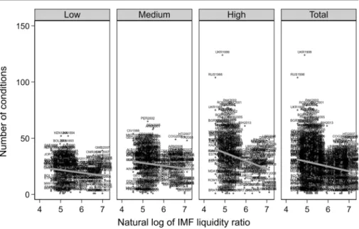
‘priority’within the IMF insofar as it relates to geopolitics or risk aversion. For instance, geopolitically important countries have greater bargaining power and may thus receive fewer conditions on average than less geopolitically important countries (Stone,2002, 2011). If the elasticity of conditionality with regard to the IMF budget constraint also depends on political priority, such that low-priority countries see their conditionality increase faster than high-priority countries when IMF resources become scarce, then the exclusion criterion would be violated through the correlation between the instrument and the unobserved variable‘priority’. To test if this is the case, in Fig.2we divide countries into low, medium, and high conditionality groups and graph the IMF liquidity ratio against the number of conditions assigned to a specific country for each year of IMF participation. Countries at different burdens of conditionality have, on average, a similar propensity of receiving more conditions when the amount of countries in IMF programs increases, as indicated by equivalent gradients of the lines of best fit across conditionality groups (all betweenr =−.15andr =−.29). We thus show that the elasticity of condi-tionality with respect to geopolitical importance is approximately constant; that is to say, the instrument satisfies the homogeneity of treatment assumption necessary for the exclusion criterion to be valid (Hainmueller et al.2016).
Finally, since the above approach is akin to a difference-in-difference design, non-parallel trends across groups with different exposure would undermine identification (Christian and Barrett2017). In our case, trends over time in the number of IMF conditions and the outcome variable should be similar across above-mean conditionality exposure and below-mean conditionality exposure groups of countries. In addition, inference would be threatened if there was a non-linear trend in the time-varying part of the compound instrument that is similar to the respective trends in the potentially endogenous variable and the outcome variable in the high-exposure group of countries. This is because such non-linear parallel trends would create spurious correlation not controlled for by year fixed effects unless the same non-linear trends are also present among the low-exposure group of
countries (Christian and Barrett2017). In our case, we would be concerned about similarly shaped non-linear trends in the IMF liquidity ratio, the number of IMF conditions, and education expenditure if these trends only occur among high-exposure countries but not the low-exposure countries. We graphically assess these two conditions below.
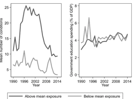
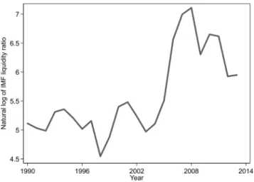
Figure3 allows us to compare trending behavior across exposure groups for the mean number of conditions (left panel) and our outcome variable of government education spending as a share of GDP (right panel). The trend pattern for the number of conditions is qualitatively similar across groups, although the high-exposure countries face a higher number of conditions by definitional fiat in any given year. We also find similar trends across exposure groups in the outcome variable. In Fig. 4, we present the temporal evolution of the IMF liquidity ratio. Here we observe no similar (non-linear) trends between the IMF liquidity ratio and the mean number of conditions, or between the IMF liquidity ratio and education expenditures. Consequently, there is no apparent violation of the design assump-tions of the difference-in-difference approach.
Fig. 2 IMF liquidity ratio and number of conditions per country-year for low, medium, and high condition-ality countries, 1990–2014. Notes: Excludes country-years without a condition. Countries divided into three equal groups based on a country’s average number of conditions per year of IMF participation. Low conditionality (0 to 25.9 conditions) countries includes Antigua and Barbuda, Barbados, Benin, Bolivia, Burkina Faso, Cameroon, Central African Republic, Colombia, Comoros, Czech Republic, Djibouti, El Salvador, Ethiopia, Gambia, Grenada, Guatemala, Guinea-Bissau, Hungary, Iceland, India, Ireland, Jordan, Kenya, Korea Rep., Kosovo, Lesotho, Malawi, Mali, Mozambique, Niger, Nigeria, Panama, Poland, Portugal, Slovak Republic, Sri Lanka, St. Kitts and Nevis, Tanzania, Togo, Tunisia, Zimbabwe. Medium conditionality (25.9 to 30.9) includes Afghanistan, Albania, Algeria, Angola, Argentina, Armenia, Bangladesh, Burundi, Cabo Verde, Cambodia, Congo Rep., Cote d’Ivoire, Cyprus, Dominica, Equatorial Guinea, Gabon, Georgia, Ghana, Guyana, Haiti, Honduras, Macedonia, Madagascar, Maldives, Mexico, Mongolia, Nicaragua, Papua New Guinea, Peru, Philippines, Sao Tome and Principe, Senegal, Seychelles, Solomon Islands, Trinidad and Tobago, Uganda, Uruguay, Zambia. High conditionality (30.9 to 62.7) includes Azerbaijan, Belarus, Bosnia and Herzegovina, Brazil, Bulgaria, Chad, Congo Dem. Rep., Costa Rica, Croatia, Dominican Republic, Ecuador, Egypt, Estonia, Greece, Guinea, Indonesia, Iraq, Jamaica, Kazakhstan, Kyrgyz Republic, Lao, Latvia, Lithuania, Mauritania, Moldova, Nepal, Pakistan, Paraguay, Romania, Russia, Rwanda, Serbia, Sierra Leone, Tajikistan, Turkey, Ukraine, Uzbekistan, Venezuela, Vietnam, Yemen
Overall, we believe that the argument for using the interaction of the within-country average of the number of conditions and the year-on-year IMF budget constraint as an instrument is well grounded. To violate the exogeneity assumption, one would have to find an unobserved variable driving the relationship between the time-variant IMF budget constraint and the outcome of interest; and such an unobserved variable would also need to be correlated with the country-specific average of conditionality after controlling for country and year fixed effects and a vector of controls. Although it is unlikely that such a variable exists, we consider this possibility by incorporating plausible candidate variables for our particular outcome of interest as additional controls in robustness checks, namely education commitments of overseas development assis-tance and the number of role-equivalent countries participating in IMF programs in the past three years. Furthermore, to violate the parallel and non-overlapping trends as-sumptions, the contemporaneous trends in the outcome of interest would have to follow different patterns across groups of countries with high compared to low exposure to IMF conditionality, and the trends in the IMF’s budget constraint, IMF conditionality, and the outcome of interest would need to overlap (Christian and Barrett2017).
Excludable instruments are also needed to account for endogeneity of IMF partic-ipation. As described in Section 2.2, past studies usually rely on UNGA voting similarity with the US (Dreher and Gassebner 2012; Steinwand and Stone 2008; Woo2013), but the LATE of the instrument might not be generalizable since politically motivated programs could be less (or more) effective (Dreher et al. 2018). Our preferred approach is thus to use another compound excludable instrument initially proposed by Lang (2016) and adopted more recently by Nelson and Wallace (2017): the interaction of the within-country average of IMF program participation across the period of interest with the year-on-year IMF’s budget constraint, again using the natural log of the IMF liquidity ratio as a proxy.
Formally specified, the predicted values for IMF participation specified in Equation (1) are derived as follows:
d IMFPROGit ¼y1 IMFPROGi IMFBUDGt þy2Xitþμiþδt ð5Þ
Here, i is country and t is year.IMFPROGd it is the predicted probability of IMF
participation;IMFPROG is the country-specific average of participation;IMFBUDG is the budget constraint of the IMF in yeart;Xis a list of covariates from the outcome equation;μis a set of country dummies; andδis a set of year dummies.
Lang (2016) provides a robust defense of the instrument’s excludability, which follows the same logic as our IMF conditionality instrument vis-à-vis the exogenous variation of the budget constraint. Again, since such an approach is akin to a (continuous) difference-in-difference design, we check below whether its underlying assumptions hold.
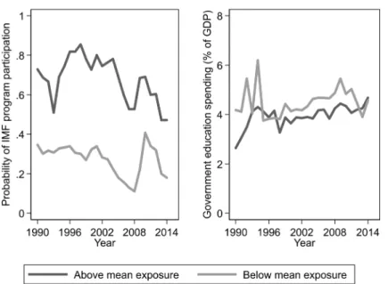
In Fig.5, we find both exposure groups to be similar in terms of their trending patterns with respect to the outcome variable and the mean probability of IMF program partici-pation. Furthermore, there is no apparent trend similarity between the IMF’s budget constraint (see Fig. 4) and the mean probability of IMF program participation and education expenditure, respectively, among above-mean participation exposure countries.
3.3 Performance assessment of estimators using Monte Carlo simulation
While the proposed multi-equation approach with correlated errors is preferable on a theoretical basis, its performance relative to alternative approaches needs to be tested. We conduct Monte Carlo simulations, which enable us to control the data generating process and thereby assess how well different estimation methods approximate the true parameter values.
Building on our theoretical discussion, we compare the performance of six estima-tors: our favored double-instrumental variable maximum-likelihood estimator that essentially linearizes the IMF participation equation to include fixed effects, akin to a 3SLS estimator, which accounts for endogeneity of IMF programs and conditionality (IV/IV/MLE); a conditional mixed process maximum-likelihood estimator that Fig. 4 IMF liquidity ratio across time, 1990–2014
accounts for endogeneity of IMF programs and conditionality but does not linearize the IMF participation equation (CFA/IV/MLE); a two-step variant of Heckman estimator using a control function approach without correcting for endogeneity of conditionality (CFA/−/OLS); a 2SLS estimator correcting for endogeneity of IMF programs through a linearized IMF selection equation but with no correction for conditionality (IV/−/OLS); a 2SLS estimator without endogeneity correction for programs but with correction for endogeneity of conditionality through an instrumental variable approach (−/IV/OLS); and a simple OLS estimator without any endogeneity correction (−/−/OLS). We scrutinize these estimators across several scenarios. In the first five scenarios, we match the proposed data-generation process but vary cross-equation correlations and the strength of the instruments. In the last two scenarios, we probe robustness of the estimators to omitted-variable bias that jointly affects IMF treatments and the outcome of interest. For each simulation scenario, the data are generated and models estimated 500 times, and three quantities are calculated: bias, root mean square error, and optimism (Bell and Jones2015).18
We find that our proposed solution—instrumenting for both IMF treatments in a multi-equation framework with joint error structure—is the preferred one unless instru-ments are weak. Whether CFA/IV/MLE is preferable to IV/IV/MLE, however, depends on the specific parameterization. For example, CFA/IV/MLE performs best when a strong instrument for IMF conditions is available, when there is high residual correla-tion across equacorrela-tions, and when the model is misspecified by ignoring a confounder
18
We implement the simulation as follows. First, in each replication loop, we create a rectangular dataset of 1000 observations. Second, we generate the normally-distributed predictors, instruments, and errors, and calculate the response variables. The instrument is defined such that it correlates with the main predictor but also includes white noise, which simulates instrument weakness. Third, we run the analysis using six different estimators in each of the seven scenarios, calculating for each coefficient estimate its bias, mean squared error, and optimism with respect to the true parameter. For detailed descriptions and results tables please refer to the
online appendices.