Discussion Papers in Economics
Department of Economics and Related Studies University of York
Heslington York, YO10 5DD
No. 11/20
Housing Debt and Consumption
By
Housing Debt and Consumption
Viola Angeliniyand Peter SimmonszOctober 2011
Abstract
The interaction between housing wealth, the …nancial portfolio of the consumer and consumption is a live issue. Life cycle models with closed form solutions under uncertainty are hard to …nd. In this paper we …nd analytical solutions for the e¤ects of house price uncertainty and employment risk on consumption, savings and mortgage …nance in a …nite horizon life-cycle model. In each period the consumer decides whether to withdraw equity from the house or not, subject to a transaction cost and a constraint on the maximum mortgage loan to value ratio. Despite risk aversion we …nd that, if borrowing is allowed in the …nancial asset, the prime portfolio e¤ect is the spread between the interest rate and the mortgage rate. House price uncertainty has an ambiguous e¤ect on consumption, which depends on the interest rate di¤erential and house price expectations since future house prices a¤ect future remortgage possibilities. If unsecured debt is not possible, we …nd that the possibility of future liquidity constraints can reduce mortgage borrowing below the maximum possible.
Keywords: precautionary savings, employment risk, mortgages, housing JEL No: D11, D14, E21
Comments on an earlier version of this paper from participants at the Copenhagen Workshop on Household Choice of Consumption, Housing and Portfolios and seminars in Padua are gratefully acknowledged. We wish to thank Martin Browning, Chris Carroll and Guglielmo Weber for useful suggestions. The usual disclaimer applies.
yUniversity of Groningen and Netspar.
zCorresponding author: Department of Economics, University of York, YO10 5DD York, United Kingdom.
1
Introduction
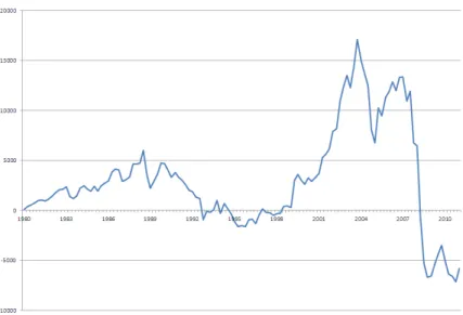
Housing is one of the major spending and …nancial decisions facing consumers. In the UK the owner occupation rate is 70%1 and housing is one of the few spending decisions that has a speci…c asset to assist its …nancing: the mortgage. In addition, for the majority of consumers wealth largely consists of housing and pension wealth. Since the latter is usually untouchable, the ‡exible part of wealth is primarily housing equity. Thus, our key argument is that most cash-convertible wealth increases are in housing wealth - pension wealth is not realisable and most households have quite negligible average values of …nancial assets. In the context of a life cycle model the realisation of wealth accruals is driven by the desire to smooth consumption. However, since consumers need somewhere to live, increases in housing wealth can only be realised to a limited extent, mainly in three ways: either by trading down house quality, by moving into rented accommodation or by remortgaging. In this paper we focus on the last one. Our view is reinforced by the policy concern over the importance of housing equity withdrawal as a means of …nancing consumption sprees, which may then lead to lack of macroeconomic control of the economy. Of course the reverse side of the coin is the prospect of falls in house prices and, thus, in housing wealth, in which case housing debt can lead to consumers being locked into negative equity. Therefore, housing wealth and equity are major drivers of consumption. Figure 1 shows that in the 1990s housing borrowing secured against housing had risen by a substantially larger amount than that needed to fund new housing investment. This trend has reversed in 2008 when, due to the …nancial crisis, housing equity withdrawal has become negative for the …rst time in the last three decades, partly due to the fall in high loan-to-value new borrowing.
To analyse the e¤ects of house price uncertainty and mortgage equity withdrawal on con-sumption, we use a real model with a time additive utility over a …nite horizon and a positive rate of time preference. The individual has a portfolio composed of two …nancial assets: a mortgage and a riskless asset. The mortgage is an adjustable rate loan that is taken for the remaining life of the consumer but can be increased at any date. In the mortgage market there are two imperfections: re…nancing the mortgage involves the payment of a …xed transaction cost and the new loan can never exceed the latest realised house price. In the last period of the life the house is sold and any outstanding debt must be paid o¤. In the model we include both
1
Figure 1: Housing equity withdrawal 1980-2011. Source: Bank of England.
employment and real house price risk, while wages and real interest rates are time varying and driven by stochastic processes, but they are foreseen by the individual
The new features of our framework (which in some respects is very stylised) are:
We explicitly model housing equity withdrawal through remortgaging as house prices change in an environment in which decisions are taken under house price uncertainty and employment risk.
There is no approximation in our approach; some variables are perfectly foreseen by the decision maker but others, such as house prices and employment status, are not, and despite this we derive a closed form analytical solution for optimal equity withdrawal and consumption.
The result is a consumption function in which the current and random values of future house prices play a critical role. On the one hand, uncertain future house prices give the opportunity of high prices and so the chance of high future equity withdrawal, reducing the need for current bu¤er stock savings against future employment uncertainty. On the other hand, there is a risk that future house prices might be low, constraining the re…nancing possibilities, which serves to depress current consumption. Which of these two e¤ects dominate depends on the interest rate di¤erential and house price expectations. We also …nd a …nancial portfolio decision important in …nancing consumption. If we
have a recontractible one period mortgage and a one period bond, then with no saving or borrowing constraints in the bond, there is an issue of whether the consumer should …nance consumption from bond borrowing or from remortgaging when housing wealth increases. We show that, despite any degree of risk aversion, with the preferences that we use, consumers will choose the cheapest …nancial source to …nance consumption smoothing as housing wealth rises. The picture is more complicated in the presence of binding liquidity constraints. We show that in this case re…nancing is possible even when the mortgage rate is relatively high. This result is consistent with a stream of the literature (Hurst and Sta¤ord, 2004; Smith and Vass, 2004) that shows that the extent to which investors do re…nance depends on the amount of liquid assets they hold.
There are special end of life e¤ects. Consumers cannot die in debt so any outstanding mortgage must be paid o¤ by current realisable wealth. But there is a cleft stick: in the …nal period of life, house prices might jump to high levels leading to large unanticipated wealth increases, or they could fall leading to the need to …nd some …nancial way of paying o¤ any existing mortgage debt outside of the value of the house.
The plan of the paper is to review the literature in section 2, give the assumptions in section 3 and derive the overall value function explicitly in sections 4. In section 5 we analytically derive the consumption function. In section 6 we present the case with liquidity constraints. We then brie‡y discuss extensions and conclude.
2
Literature Review
Housing impacts on individuals in various ways. One strand of the literature focuses on the role of housing on portfolio decisions. Some economies have a liquid rental market for housing and an illiquid retail market; others have a negligible rental market outside metropolitan areas but an active retail market (Chiuri and Jappelli, 2001). Flavin and Yamashita (2003) stress that with a thin rental market housing decisions have to balance …nancial asset portfolio considerations with the need for housing services. In the UK about 43% of homeowners bought their house outright without a mortgage and home equity accounts for about 60% of personal wealth (Banks et al., 2003). Thus owner occupiers face the risk of random house prices - both nominal and real. Several authors have argued that this risk explains why consumers do not invest in equities
but in relatively safe assets: their overall portfolio including housing has the right balance of risk and return without investing in equities (Pelizzon and Weber, 2008). On the other hand, 57% of house buyers do have a mortgage and for them there are additional risks: the liquidity risk that with a bad income shock it would be di¢ cult to maintain repayments (Fratantoni, 2001) and the risk that the mortgage interest rate might change. In addition, they have to make other decisions: when to repay the mortgage or, in common with the …rst group who have no mortgage, when to withdraw equity from the house. Furthermore, both of these groups face common shocks, such as wage and employment risk. The importance of these di¤erent risks varies over the life cycle; usually for highly geared young households, with housing debt a high proportion of wealth and income (Cocco, 2005), the liquidity risk is higher than for older households with, on average, more diversi…ed wealth and more house equity. This implies that the typical life cycle portfolio composition sees systematic changes in the share of housing in wealth.
There is also a recent literature that looks at the collateral/bu¤er stock e¤ect of housing investment on precautionary savings. The argument is that, although the retail housing market is illiquid, housing equity serves as a bu¤er stock of wealth against low probability but very negative income shocks. Thus, even if housing is rarely traded because of the high transaction costs, it allows a higher level of mean consumption since if the worst income events occur there is a bu¤er stock of wealth that can be realised. And, if trend real houses prices are growing then housing wealth is rising which may allow households to cut back …nancial asset saving (Berry et al., 2009). Benito (2009) …nds that housing equity acts as a bu¤er stock against bad shocks, e.g. in employment in the UK. However the bu¤er role of housing wealth must be o¤set against the fact that most homeowners hold mortgage debt against their housing (Campbell and Cocco, 2003), so that net housing wealth may be quite low, and also the fact that consumers need a roof over their head, so that they might not be able to sell the house where they live and, even if they can, they have to buy or rent another one. In the presence of high transaction costs in housing and a thin rental market, consumers can withdraw equity from their properties by using the bu¤er stock of housing wealth. This is predominantly executed by remortgaging. However, mortgage markets are imperfect in that there are costs in altering the debt position and limits on the amount that can be borrowed in a mortgage. This means that there may be inertia in the re…nancing decision. For example, in the US, where most mortgages are at …xed nominal interest rates, there is active re…nancing as interest rates change (Majumdar, 2004),
but in Europe this is less common (Smith and Vass, 2004). Even in the US there is evidence of suboptimal timing e¤ects (Agarwalet al., 2009; Campbell, 2006).
Housing wealth interacts with unsecured borrowing. In itself housing wealth provides col-lateral against loans for non-housing purposes. Unsecured borrowing constraints may lead to equity withdrawal to …nance consumption (Benito & Mumtaz, 2009), although the ‡ip side of this is that negative home equity may lead to unsecured borrowing (Iacoviello, 2004). Disney et al. (2010) …nd some evidence of both in the UK.
Another issue in the literature is related to the degree of substitutability of housing and …nancial wealth in determining consumption. Will two households with the same aggregate wealth, the same labour income prospects and the same preferences follow the same consump-tion funcconsump-tion if one of them has a much higher proporconsump-tion of housing wealth than the other? The empirical results here are mixed (Hoynes and McFadden, 1996; Bosticet al. 2009; Majum-dar, 2004). Similarly Attanasio et al. (2009) and Browning et al (2010) do not …nd e¤ects on consumption of housing as a special form of wealth although there is some evidence of its role as a source of collateral. The question is important since consumer spending ‡uctuations are often seen as an important determinant of business cycle ‡uctuations. The main transmission mechanism for converting changes in housing wealth into disposable resources is the mortgage; therefore, analysing how mortgage decisions are made is crucial. The paper of Campbell and Cocco (2003) is a related major study of the relative advantages of …xed and variable rate mortgages that is close to our concerns. Li and Yao (2007) also study the e¤ects of house price changes on household consumption. However, their analysis substantially di¤ers from ours in that all mortgage re…nances in their model are for consumption purposes only and are not driven by …nancial e¢ ciency considerations; this arises from the assumption that the unsecured and secured borrowing rate are set to be equal. Remortgaging and equity withdrawal is one of the main ways in which housing wealth can …nance other household choices. Some empir-ical work reinforces our theoretempir-ical results: Canner et al. (2002), Schwarz et al. (2008) and Ebner (2010) …nd that …nancial e¢ ciency factors are important in determining remortgaging and Agarwalet al. (2006) and Campbell (2006) also give these factors a major role.
With its complex features, modelling these housing choices is not straightforward. Quite special assumptions are necessary to derive analytical conclusions; for example Ortalo-Magné and Rady (2006) use utility linear in consumption, a …xed utility premium for a large house over a smaller one and no uncertainty and derive analytical results about the nature of general
equilibrium house prices. Campbell and Cocco (2003), Cocco (2005), Li and Yao (2007) and Yang (2009) rely on calibrated numerical simulation involving grid search over both their state and control variables to derive the optimum. This approach allows the use of more general assumptions about the stochastic processes that drive house prices, interest rates and labour income but does not yield analytical conclusions.
3
The Model Assumptions
We consider a …nite horizon T of discrete time periodst. Within a periodt < T the timing of the model is as follows. At the start of the period the individual has a portfolio composed of two …nancial assets: a riskless assetAt with rate of return rt and a mortgage Mt that allows
the investor to borrow against the value of the house at a rate t. We assume that both rt
and t are perfectly foreseen and that a mortgage loan initiated at t matures at T. In each period, consumers decide whether to re…nance or not. When re…nancing occurs, they redeem the existing debt, pay a transaction costkand choose a new mortgage sizeMt+1, which cannot
exceed a fraction of the latest realised pricept. The loan to value ratio (LTV) is a key statistic
used by lenders and regulators in the UK. For example the Financial Services Authority reports that in 2010 more than 70% of new mortgages had LTV below75%and less than2%had LTV above 90%. House prices are stationary with a deterministic trend. Then, consumption ct is
chosen and next the individual receives labour incomewts: if the individual has a job, this is the wagewt, if she is unemployed, it is bene…tsBt:Each period there is a constant probabilityaof
being unemployed and wages and bene…ts are time dependent but perfectly foreseen. Finally, the stock of …nancial assets At+1 to carry forward into the next period is determined. This
means that assets bear all the e¤ects of shocks in employment, but this only a¤ects the current period and is insigni…cant over the lifetime2. Note also that as viewed from earlier periodsMt+1
is random, since it depends on the realisation of random house prices through the constraint Mt+1 pt:
The general form of the budget constraint in any period before the …nal one is
At+1= (1 +rt)At+wts+Mt+1 (1 + t)Mt k ct
2This is unimportant and arises from the de…nition of the period, but the use of this timing simpli…es the
t-1 t t+1
At,Mt rtAt ∆M,ρtMt ct et/ut
Figure 2: Timing
If there is no re…nancingMt+1=Mt and no transaction cost has to be paid (k= 0):
At+1= (1 +rt)At+wts tMt ct
The consumer enters the …nal period with mortgage debtMT;…nancial assets AT and with a
realised house price of pT. At the period start the individual sells the house (but arranges to
continue living in it for the duration of the period3), redeems any outstanding mortgage and consumes all the known cash on hand.
cT = (1 +rt)AT +pT +wTs (1 + T)MT k
We also assume that in the last period for sure the individual is unemployed (but we could also think of this as retirement) so that wsT = BT: This is without loss of generality since
consumption is determined prior to knowledge of employment status and then in the last period it would have to be reined back to a level that will prove feasible if it turns out that the individual is unemployed, as it is impossible to die in debt.
Lifetime preferences are additive and there is a positive intertemporal discount rate :4
U0= tu(ct)
3
There is a small market in which equity in the house can be realised in the last years of life eg by selling the house to a …nancial institution and buying back an option to live in it until death but this is not very well developed.
4
It would be very simple to add a bequest motive, especially if the utility of bequests also has an exponential form.
The per-period utility function has a CARA form and depends only on consumption:
u(ct) = 1 exp( bct)
wherebis the coe¢ cient of absolute risk aversion. That is, there is a zero utility of housing and an inelastic labour supply. Since we assume that the individual keeps the house throughout her life, then omitting it from the value function is without loss of generality. Ignoring the disutility of work is more serious and is based on simplicity; we could include it assuming that jobs have …xed hours of work. Similarly, we could incorporate socio-demographic variables, such as the number of children into the analysis. CARA preferences have the advantage of exhibiting prudence and allowing us to derive exact solutions without having to approximate Euler equations. Much of the literature works with isoelastic felicity, which generally requires approximation to get solutions. On the one hand, there is some evidence (Gourinchas and Parker, 2002) that the approximation error involved can be substantial; on the other hand, since isoelastic preferences have unbounded marginal utility at zero consumption, they generally serve to keep cash on hand positive and, therefore, almost act like a liquidity constraint. With CARA, marginal utility is …nite at zero consumption, so we may expect to see the consumer actively borrowing. However, the lifetime budget constraint prevents her dying in debt.
The overall optimisation problem has the form
max T X t=1 t[1 exp( bc t)] subject to At+1 = (1 +rt)At+wts+Mt+1 (1 + t)Mt k ct Mt+1 > Mt; t < T At+1 = (1 +rt)At+wts tMt k ct Mt+1=Mt; t < T cT = (1 +rt)AT +pT +BT (1 + T)MT k Mt Mt+1 pt
The interesting empirical questions about mortgage re…nance concern equity withdrawal and portfolio diversi…cation among housing assets, mortgage debt and net …nancial assets. There are two reasons primarily for mortgage re…nancing. The …rst motivation is that bank borrowing might get very cheap relative to mortgage debt in which case the consumer may wish to switch from secured to unsecured debt so far as this is allowed. The second reason for
re…nancing is that as house prices and, thus, wealth rise, the individual may want to withdraw equity from the house by increasing the mortgage. To focus on the latter we impose the constraint that Mt Mt+1 and assume that the individual starts life with a given mortgage
M1: Our argument is that consumers will only wish to reduce their mortgage debt if there is
an unanticipated income gain large enough so that consumption smoothing bene…ts overcome the transaction cost that has to be paid to reduce the mortgage. In practice in the reality this does not happen - it is con…ned to a tiny proportion of the population who receive large lump sum income gains, e.g. winning the national lottery or large bequests from wealthy relatives. Hence, we argue that the constraint Mt Mt+1 pt captures the essence of housing equity
withdrawal combined with lender limits on the extent to which this is possible.
4
Value Function
In any periodt < T the value function is the maximum of the value function with re…nancing and the value function without any mortgage re…nancing:
Vt= max VtR; VtN R
Based on Merton (1992), and Berlo¤a and Simmons (2003), we conjecture that Vt takes the
form:
Vt(At; Mt; pt) = t texpf b t[(1 +rt)At (1 + t)Mt]g (1)
The …rst main result of our paper is to derive this form and the functions ; ; . In fact, will prove to be a discounting function depending on the rate of time preference and a discounting function depending on interest rates. The most interesting function is , which depends on the expectation of future house prices and employment states and on the future optimal mortgage and saving decisions.
In periods before the …nal one (in which re…nancing does not occur) the form of the value function depends on whether it is optimal to undertake re…nancing. We derive the value functions at twith and without re…nancing and then compare them to determine the optimal re…nancing decision.
re…nancing is VtR(At) = 1 + t+1 [ (E t+1) t+1(1 +rt+1)]1=[1+ t+1(1+rt+1)] expf b t[(1 +rt)At (1 + t)Mt]gWt exp b t[Mt+1 k Mt+1(1 + t+1)=(1 +rt+1)] = t where Wt=faexp [ b t+1(1 +rt+1)wt] + (1 a) exp [ b t+1(1 +rt+1)Bt]g1=[1+ t+1(1+rt+1)]
is the expected utility term corresponding to next periods labour income and:
t= t+1
(1 +rt+1) 1 + t+1(1 +rt+1)
is the "discounted future interest rate".
At the start of t; given that remortgaging takes place, the mortgage re…nancing decision is to choose Mt+1 to maximise VtR(At) within the constraint Mt Mt+1 pt. De…ning
t+1 = 1 1 + t+1 =(1 +rt+1), this is equivalent to minimising:
exp ( b tMt+1 t+1)
The decision rule is then:
Mt+1 = pt if t+1 >0
Mt+1 = Mt if t+1 <0
Therefore, re…nancing occurs only when t > 0 (i.e.rt+1 > t+1) and the individual chooses
maximum equity withdrawal. Integrating this into the value function
VtR(At) = 1 + t+1 [ (E t+1) t+1(1 +rt+1)]1=[1+t+1(1+rt+1)]
expf b t[(1 +rt)At (1 + t)Mt]g exp b t max( t+1;0) pt
k t+1 exp b t max( t+1;0) Mt k t+1 Wt= t
Similar arguments show that without re…nancing
VtN R(At) = 1 + t+1 [ (E t+1) t+1(1 +rt+1)]1=[1+ t+1(1+rt+1)] expf b t[(1 +rt)At Mt]g exp( b t t+1Mt) Wt= t
By comparing the two value functions we obtain the condition under which re…nancing occurs. At tthe individual chooses to re…nance the mortgage ifVtR(At)> VtN R(At).
If t+1 >0(the mortgage rate is lower than the interest rate) then re…nancing occurs when
pt Mt>
k
t+1
In terms of the debt service costs it pays to re…nance to the highest extent possible by setting Mt+1 =pt so long as the interest gain on the sum involved more than covers the transaction
cost of re…nancing.
On the other hand, if t+1 < 0 (the mortgage rate is higher than the interest rate), no
re…nancing occurs.
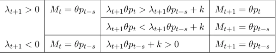
We can summarise the possible remortgage actions at time t(assuming that at some past point t sa maximum mortgage had been taken) as
t+1 >0 Mt= pt s t+1 pt> t+1 pt s+k Mt+1 = pt t+1 pt< t+1 pt s+k Mt+1 = pt s t+1 <0 Mt= pt s t+1 pt s+k >0 Mt+1 = pt s
Table 1: Possible remortgage actions
4.1 Overall Value Function
The overall value function is the larger of VtR(At; Mt) and VtN R(At; Mt), which gives us the
result
Proposition 1 The value function has the form5
Vt(At; Mt; pt) = t texpf b t[(1 +rt)At (1 + t)Mt]g
5
In fact the value function has this same form (with a di¤erent de…nition of ) if is stochastic andkis time varying or stochastic as long as the current period mortgage rate and transaction cost are realised prior to the current re…nancing decision.
where t; t; t are de…ned recursively through t = 1 + t+1 (2) t = t= t+1 (1 +rt+1) 1 + t+1(1 +rt+1) (3) t = (E t+1) t 1 t 1 t Wt= texp [b tmax ( t+1;0)Mt] (4)
exp b t max ( t+1;0) max pt
k
t+1
; Mt
Solving the recurrence relations for tand t
aT t = t X s=0 s T t = s=t 1 s=0 (1 +rT s) 1 + t=01 ss==0(1 +rT s)
The recurrence relation in , which captures the e¤ect of future house prices and employ-ment uncertainty, requires some careful analysis.
4.2 E t+1 : The E¤ects of Future House Price Uncertainty
Future house prices (pt+2; pt+3::) and the current remortage decision Mt+1 determine the
op-portunities and desirability of future re…nancing. It is through this channel that house price uncertainty impacts on current decisions. In our model, the e¤ects of future house price un-certainty at time t work through the expression Et t+1:However, since the mortgage is only
binding for a single period (next period there is another re…nancing point) and we have assumed that any trend in pt is not stochastic, it is only immediate future house prices that impact on
the Mt+1 decision. Therefore, Et+1 t+2 is not a function of pt+1 and at time t the random
term in t+1 is:
Ft+1 = exp b t+1 max ( t+2;0) max pt+1
k
t+2
; Mt+1 (5)
where
Gt+1 = 0 if t+2<0
= t+2Mt+1 if t+2 >0 and pt+1 t+2 k < t+2Mt+1 (6) = pt+1 t+2 k if t+2>0and pt+1 t+2 k > t+2Mt+1 (7)
We want to compute EtFt+1 overpt+1:
If t+2 <0;the consumer does not wish to re…nance. In this caseGt+1 is not random, so
EtFt+1=Ft+1:
If t+2 > 0 it is more complex. The second case (6) holds when house prices are such
that the consumer potentially wishes to re…nance to the maximum permissible extent but the savings from doing so will not cover the transaction cost of re…nance. This occurs when
pt+1 < Mt+1+
k
t+2
On the contrary, in the third case (7), which holds for pt+1 above this critical value, the gains
from taking out a new maximum mortgage do cover the transaction cost. Hence when t+1>0,
if we de…ne the probability that the maximum remortgage will not cover the transaction cost by t= Pr( pt+1< Mt+1+ tk+2), the expression forEtFt+1 becomes:
EtFt+1 = Et exp [ b t+1( pt+1 t+2 k)] pt+1 > Mt+1+
k
t+2
(1 t) + exp( b t+1 t+2Mt+1) t
Suppose that the support of the distribution ofpt+1 is [pt+1; pt+1]:
if Mt+1+ k t+2 < pt+1 then t= 0 if Mt+1+ k t+2 > pt+1 then t= 1
Therefore, we have two boundary cases where either house prices are always so low that a maximum equity withdrawal will not cover the transaction cost or they are so high that with certainty the maximum remortgage is pro…table. Table 2 summarises the various forms of
EtFt+1:Since Et t+1= (Et+1 t+2) t+1 1 t+1 1 t+1 EtFt+1Wt+1= t+1 (8)
the nature of Et t+1 follows. Thus, there are only e¤ects of immediate future house price uncertainty on the current value function if t+2 > 0 In fact, extending this argument, the
distribution of house prices at any future date only a¤ects the current value function for those periods in which +1>0. Appendix A.2 shows that6:
t = (ET 1 T)(1 t)(1 t+1)::(1 T 1) (9) 1 t 1 t 1 t+1 (1 t)(1 t+1) ::: 1 T 1 (1 t)(1 t+1)::(1 T 1) Ft(EtFt+1)1 t(Et+1Ft+2)(1 t)(1 t+1):::(ET 2FT 1)(1 t)(1 t+1)::(1 T 1) Wt(Wt+1)1 t:::(WT 1)(1 t)(1 t+1)::(1 T 1) t t t+1(1 t) t+1 ::: T 1(1 t)(1 t+1)::(1 T 1) T 1
Note that there is an e¤ect on t of the time to go to the horizon: the longer the remaining future, the higher the number of terms in the product for since there are more future nodes. Therefore, in earlier periods tends to be higher, which re‡ects the e¤ect of the greater amount of uncertainty remaining. Conversely, towards the end of life there is little remaining uncertainty and so on these grounds less of a need for precautionary savings.
6 If the probability of unemployment was either history dependent or uncertain, then so long as it is
Et Ft +1 t +2 < 0 1 t +2 > 0 M t +1 + k t+2 < p t+1 Et exp [ b t +1 ( pt+1 t +2 k )] M t +1 + k t+2 > pt+1 exp ( b t +1 t +2 M t +1 ) p t+1 < M t +1 + k t+2 < pt+1 exp ( b t +1 t +2 M t +1 ) t + Et n exp [ b t +1 ( pt+1 t +2 k )] pt+1 > M t +1 + k t+2 o (1 t ) T able 2: E Ft +1
5
Consumption
From the relevant …rst order conditions for consumption we can derive the consumption function and examine its properties.
Proposition 2 Optimal consumption is given by
ct = 1 t b ln " E t+1 1 t # + t[(1 +rt)At (1 + t)Mt] 1 t b ln(Wt) + t max ( t+1;0) max pt k t+1 ; Mt max ( t+1;0)Mt
This expression subsumes two cases: when t+1>0and pt t+1 k > Mt t+1the individual
chooses to re…nance at t, whereas when t+1 > 0 and pt t+1 k < Mt t+1 or t+1 < 0
optimally there is no re…nance. The main features of the consumption function are summarised by proposition 3.
Proposition 3 Uncertainty of future house prices may raise or lower current consumption. If (a) t+2 >0 and pt+1 t+2 k > Mt+1 t+2 optimal consumption under uncertain house
prices is lower than with house price certainty.
(b) t+2 > 0 and Etpt+1 t+2 k > Mt+1 t+2 uncertainty in house prices may raise or
lower consumption depending on the nature of the house price distribution, the interest rates and the degree of risk aversion
(c) t+2 >0 and Etpt+1 t+2 k < Mt+1 t+2 optimal consumption under uncertain house
prices is higher than with house price certainty and precautionary savings are negative.
Proof. See the appendix.
Both with and without re…nancing the e¤ect of future period employment risk and house price uncertainty is to shift the intercept of the consumption function by an amount that de-pends on the degree of risk aversion. Since it is possible that Et t+1 <1 t, the future
uncertainty in house prices may actually increase rather than reduce consumption. Uncertain future house prices give the opportunity of high prices and so the chance of high future eq-uity withdrawal, reducing the need for current bu¤er stock savings against future employment uncertainty. If future house prices are certain, then the expression for Et t+1 changes when
t+2 >0:We can gauge the e¤ect of this by comparingEt t+1with its value when house prices
house prices the consumer has the same expected re…nancing possibilities; this is the standard case in which uncertainty lowers current consumption unambiguously and precautionary sav-ings are positive. In (b) on the one hand there is a risk that future house prices might be low, constraining the re…nancing possibilities, which serves to depress current consumption; on the other hand, house prices might be high, giving the opportunity of future equity withdrawal, higher than with certain house prices. The overall e¤ect is ambiguous and depends on future house price expectations. The ambiguity exists even though we do not have any stochastic trend in house prices. If we had, this result would be even stronger. Finally in (c), when with certain future house prices no re…nancing is undertaken ( Etpt+1 t+1 k < Mt+1 t+1),
precau-tionary savings are negative and house price uncertainty serves to raise current consumption. The intuition is that in this case house price risk is just upside risk.
Summing up, in each of these cases (a)-(c) housing is acting like an intertemporal bu¤er stock of wealth with e¤ects on the current level of savings. Knowing that in the future there will be a redeemable asset (though of uncertain value), the consumer can a¤ord to borrow today. In addition, the composition of wealth between net housing wealth (pt Mt) andAthas
an impact on consumption. The marginal propensity to consume out of wealth is t(1 +rt)
but out of a reduction of the current mortgage is t(1 t+1):
Moreover, there is an e¤ect on consumption of the remaining length of the horizon. We have seen thatEt 1 t tends to fall through time and this serves to yield consumption growth
through time ceteris paribus. As time passes there is less remaining uncertainty and thus less of a need for precautionary savings.
Proposition 4 Labour income uncertainty depresses consumption and raises savings.
Proof. See the appendix.
As usual with CARA preferences, consumption is linear in net wealth(1 +rt)At Mt but
is nonlinear in expected current period labour income. The latter is essentially an artifact of the assumed within period timing where consumption has to be chosen before the employment status of the current period is realised. In fact this labour income risk reduces consumption for familiar reasons due to the risk aversion of the consumer. For current labour income this works through the expected utility of current labour earnings, for future labour income risk it works through the concavity of Et t+1 in labour incomes.
and consumption increases
When it is optimal to re…nance, the e¤ect of equity withdrawal on current consumption is unambiguously non-negative. However, with no re…nancing, a shift in the current mortgage state may increase or reduce consumption. It will have a negative e¤ect on consumption when
t+1 < 0 and a positive one when t+1 > 0 but the cost saving from increasing the current
mortgage Mt topt does not cover the transaction cost of doing so.
Remark 6 Current mortgage rates in‡uence consumption through t+1: a fall in the mortgage
rate encourages re…nance which raises consumption.
The current mortgage interest rate only has e¤ects via t+1. When t+1 >0 and pt > Mt
there is scope for increasing the mortgage so long as the interest gain covers the transaction cost. A fall in the current mortgage rate increases the chance of re…nancing and therefore may cause a switch from no re…nancing of the current mortgage to re…nancing to the maximum extent possible, which causes a jump in consumption. Only a part of the current wealth change arising from remortgaging is consumed in the current period (the coe¢ cient ), while the other part of the wealth change is used to smooth future consumption.
Remark 7 The current savings interest rate has income e¤ ects on consumption, the e¤ ects of future interest rates on savings are complex.
The current saving interest rate has obvious income e¤ects on consumption. First, there is a consumption increasing e¤ect through raising capital income when the consumer has positive …nancial assets, but a decreasing e¤ect through raising the debt service cost when assets are negative. Future savings rates and especially that of the next period have much more complex e¤ects: directly through altering the slope of the consumption function in most variables, indirectly through varying t+1 and a¤ecting the discounting terms in Et t+1: If at t the
foreseenrt+s increases (s >0)all the terms in fort < sincrease. In particular if s= 1
then t+1 is una¤ected and 1=(1 + t+1(1 +rt+1)) falls, so that the marginal propensity to
consume out of labour income expected for this period decreases.
Remark 8 An increase in risk aversion reduces the variability of consumption over time. As the degree of risk aversion rises, the absolute value of the intercept of the consump-tion funcconsump-tion falls in any period and so between any two periods there is less variability in consumption. In particular there are smaller jumps in consumption when re…nancing occurs.
6
Liquidity constraints
We have assumed that there are no restrictions on borrowing in a one period …nancial asset; the only constraint is that debt must be cleared prior to death. As long as the lifetime budget constraint is respected, consumers can borrow as much as they wish. This assumption is important in making the key determinant of the re…nancing decision the relative interest rate advantages of borrowing against the house or against future wealth (including future labour earnings and the future value of the house). Another e¤ect is that despite the risk averse preferences, the special implication of CARA is that optimal …nancial policy is essentially bang-bang, using only either mortgage or bank …nance as debt both to smooth shocks and …nance the house. Empirically this is far-fetched because, according to the Family Resources Survey, in 200412%of British households held no savings and any unsecured debt was con…ned to credit card debt. What are the implications of assuming that At 0 is a market constraint? The
re…nancing decision becomes much less transparent since it has to take account of the fact that remortgaging now in‡uences the chance with which in the next period the consumer may end up being liquidity constrained, e.g. if she loses her job. The multiperiod decision tree increases hugely in complexity since then at any period current decisions in‡uence the probability that in the next and further future periods it will be optimal to be credit constrained withAt= 0:
Even to solve for the optimal policy in this framework, let alone estimate parameters, numerical solution is necessary. And if that is the case then why use CARA or CRRA preferences? It would make more sense to use more ‡exible preferences allowing for a clear distinction between risk aversion and intertemporal substitution for example. What we can do however is highlight the new types of optimal solution phase that can arise by retaining our model assumptions but looking at just a three period example. The result is that when it is optimal to set At = 0 it
may be optimal to have a positive level of mortgage …nance below the maximum possible or even the maximum mortgage …nance possible even if the mortgage rate is high. On the other hand when optimally At > 0 it is optimal to minimise on mortgage …nance if the mortgage
rate is higher than the interest rate.
To illustrate these e¤ects, we take a special case of our framework in which the there is no re…nancing transaction cost (k= 0), = 1, there is no unemployment risk (there is a certain wage atT 1and certain bene…t income atT)and the mortgage interest rate is always above the one period …nancial asset rate r, which is a reasonable assumption in this case because r
is now the saving rate. First consider the last two periodsT and T 1:In the …nal period the individual consumes any savings held at the period start, cash in the house and repays any outstanding mortgage debt and receives social security bene…t so utility is given by
u(cT) = exp( b[pT +wT]) exp( b((1 +rT)AT (1 + T)MT))
At period T 1 the value function is then
VT 1 = 1 + ZT 1exp( b(MT AT))
exp( b((1 +rT)AT (1 + T)MT))XT 1Eexp( b[pT +wT])
where ZT 1 = exp( b[(1 +rT 1)AT 1+wT 1 (1 + T 1)MT 1]; XT 1 = Eexp( b[pT +wT])
The T 1 decision variables are AT; MT and the constraints are AT 0; MT 1 MT
pT 1: The derivatives @VT 1=@AT; @VT 1=@MT evaluated at particular points are critical in
determining the optimal decisions atT 1:These derivatives are
@VT 1=@AT = ZT 1exp( b(MT AT) + XT 1(1 +rT) exp( b((1 +rT)AT (1 + T)MT))
@VT 1=@MT = ZT 1exp( b(MT AT)) XT 1(1 + T) exp( b((1 +rT)AT (1 + T)MT))
At any time t the individual can optimally choose to be in one of four states according to the values of the derivatives above (see appendix):
(1) At>0; Mt=Mt 1
(2) At= 0; Mt=Mt 1
(3) At= 0; Mt 1 < Mt< pt 1
(4) At= 0; Mt=pt 1
The values ofZT 1 and XT 1 in relation to the current mortgage size, house value and the
two interest rates are critical in determining the optimal regime for the individual. ZT 1re‡ects
the utility from consuming periodT 1disposable resources,XT 1 re‡ects the expected utility
from consuming periodT real disposable resources. Figure (3)below shows how the parameters control the optimal choices atT 1:If ZT 1=XT 1 is su¢ ciently high the individual is credit
X
T-1 Max{(1+rT)exp(b(2+rT)pT-1, (1+rT)exp(b(2+rT)pT-1}(
1+rT)exp(b(2+rT)MT-1)
AT>0,MT=MT-1Z
T-1 AT=0,MT=pT-1(
1+rT)exp(b(2+rT)pT-1)
AT=0,Int MT AT=0,MT=MT-1Figure 3: Optimal regimes in the presence of liquidity constraints.
individual does not re…nance the mortgage but keeps it at its minimum level and also saves. Between these extremes the relation between the current house value and mortgage and the relation between the two interest rates determine whether the individual re…nances with an increased mortgage but at a level below the maximum obtainable.
The value function atT 1 is (with = 1 + and R= 1 +r) takes four possible values:
1. Ifexp( b(RT 1AT 1 T 1MT 1))> XT 1 Texp(b(wT 1+ (1 + T)pT 1)) VT 1 = 1 + exp( b RT 1 +RT (RT 1AT 1 T 1MT 1)) exp( b(wT 1+pT 1)) XT 1exp(b TpT 1) 2. If TXT 1 exp(b(wT 1+ (1 + T)pT 1))>exp( b(RT 1AT 1 T 1MT 1)) > TXT 1 exp(b(wT 1+ (1 + T)MT 1) VT 1 = 1 + exp( b T 1 + T(RT 1AT 1 T 1)MT 1) exp( b T 1 + TwT 1)( XT 1 T)) 1 1+ T 1 + T T
3. If TXT 1 exp(b(wT 1+ (1 + T)MT 1)>exp( b(RT 1AT 1 T 1MT 1)) > RTXT 1 exp(b(wT 1+ (1 + T)MT 1)) VT 1 = 1 + exp( b(RT 1AT 1 ( T 1 1)MT 1)) exp( bwT 1) XT 1exp(b TMT 1) 4. IfRTXT 1 exp(b(wT 1+ (1 + T)MT 1))>exp( b(RT 1AT 1 T 1MT 1)) VT 1 = 1 + exp( b RT 1 +RT (RT 1AT 1 T 1)MT 1) exp( b T 1 + TwT 1) ( XT 1 T)) 1 1+RT 1 +RT RT exp(b( T RT) 1 +RT MT 1)
At T 2 the decision variables areMT 1; AT 1 which are selected to maximise u(cT 2) +
ET 2VT 1: VT 1 is a piecewise continuous function with four regimes or branches VTi 1, the
probability of being in each branch i at T 1 depends on the choices made at T 2:So we can write
EVT 1= iPr(ijMT 1; AT 1)E(VTi 1jbranchioccurs)
For example for the …rst branch
Pr(i = 1jMT 1; AT 1) = Pr([ET 1exp( bpT)] exp(b(wT 1+ (1 + T)pT 1)) < exp(bBT) exp( b(RT 1AT 1 T 1MT 1)) T )
and similarly for the other branches. This demonstrates the way in which the complexity of the current decision increases with the liquidity constraints. At T 2 the choices of MT 1
and AT 1 will involve trade-o¤s between marginal value changes at T 2 and the expected
marginal value changes at T 1 over the four branches, as well as shifts in the chances that each branch occurs atT 1:Given the strictly concave within period utility used, the marginal values are nonlinear in the decision variables and analytical solution is not possible.
To summarise adding liquidity constraints means that explicit solution of the lifetime prob-lem requires simulation and calibration and hence the generality of a full analytic solution is lost. Nevertheless we can see that we would expect some individuals to be independent of
…nancial markets (M = A = 0);others to be savers with no or a minimal mortgage and yet others to not save and have either a maximum mortgage or a mortgage but at a lower level than the maximum attainable.
7
Other extensions
Our approach suggests some obvious areas for future research and has various special assump-tions whose force we try to evaluate in this section.
First, generally the amount that can be borrowed on a mortgage is limited not only by the house value but also by the current income level. The rationale for this constraint seems to be on debt service cost grounds. For example in the UK the mortgage cannot usually exceed three or four times the income. However, to incorporate the income constraint into the analytical framework would raise nothing new conceptually and it would make the algebra more complicated. Given that the individual wishes to re…nance in periodt;the new mortgage decision would be7
Mt+1 = min (pt; wt 1) if t>0
Again it is optimal to remortgage only if there is a …nancial advantage:
min (pt; wt 1) max ( t;0) k Mt t >0
By substituting this condition into the value function, we obtain the term in mortgage activity:
minfexp( b t tMt);expf b t(1 +rt+1) [max ( tmin (pt; wt 1);0) k]ggWt= t
Even in this case all the e¤ects of uncertainty are captured in , whose recurrence relation (4) becomes
t= (E t+1)
t
1 t
1 t
expf b tmax [ tMt;max ( tmin (pt; wt 1);0) k]gWt= t
Then the time path of can be easily deduced by following the methods of section 5.1. Another obvious extension would be to allow for more than one type of house, e.g. a large expensive house with price pt and a small cheaper house with price t, where both prices are
7
uncertain and t< pt. Consumers could then trade down from large to small houses and vice
versa. In terms of housing decisions, attthere are three choices: retain the existing house and mortgage, retain the existing house but re…nance, change house and re…nance. In this context it makes sense to add a second transaction cost kth that is incurred when changing house (in addition to the re…nancing transaction cost). The e¤ect is to add a third branch to the value function and the overall value function is then the maximum over the three branches. If we keep the other assumptions (especially that of no liquidity constraints), the re…nancing decision will have the same form, once any house purchase/sale has been decided. Again all uncertainty will be channelled through ;the value function will have a similar structure and the recurrence relation for (4) will become
t = [ (E t+1) t+1(1 +rt+1)]1=[1+ t+1(1+rt+1)]
expf b tmax[pt t kht + tmax ( t;0) k; tMt; ptmax ( t;0) k]gWt= t
Furthermore, in the compulsory retirement case we could make the date of retirement uncertain. This is similar to dropping the perfect foresight assumption on wages and has signi…cant e¤ects (see Berlo¤a and Simmons, 2003, and below).
The main special assumptions that we have made are:
CARA preferences depending only on consumption and independent of housing or leisure or socio-demographics.
A problem with CARA is that optimal consumption may turn out to be negative since marginal utility is …nite at zero consumption. We could make the utility vary with housing and leisure; in the context of a model with a single indivisible house type, the former would add little, but the latter would be interesting and, although most of the structure of the value function, the re…nancing decision and consumption would remain unchanged, there would be some additional preference e¤ects (see Berlo¤a and Simmons, 2003).
With general strictly concave preferences over just consumption u(ct); the re…nancing
problem at tcan be written as
Vt= maxu(ct) +EV((1 +rt+1)At+1 (1 + t+1)Mt+1)
or using the budget constraint with Zt= (1 +rt)At (1 + t)Mt+wst k
maxu(ct) +EV((1 +rt+1)(Zt ct) + (1 +rt+1)Mt+1 (1 + t+1)Mt+1)
Ifctis set at its optimal level from the envelope theorem inctthe marginal value ofMt+1
is
@Vt=@Mt+1 =EV0()(rt+1 t+1)
With CARA this generates a corner solution inMt+1 but with general preferencesEV0()
varies nonlinearly withMt+1.
Perfect foresight of unemployment bene…t, wage and interest rates.
This is an important simpli…cation with potentially large implications. If interest rates are uncertain, the consumer has a real portfolio choice, not just a choice driven by the asset with the highest return. We might then expect to get some diversi…cation of the portfolio depending on the covariance between the interest rates and the covariance be-tween interest rates and house prices.
Uncertainty in the real wage when employed can readily be incorporated so long as it is uncorrelated with house prices and with the chance of having a job. The value function, the re…nancing decision and consumption will have a similar functional structure where the expected labour income termWtbecomes
Wt=aEtexp( b t+1(1 +rt+1)wt) + (1 a) exp( b t+1(1 +rt+1)Bt)
If there is correlation between house prices and wages it is more complex. Another assumption we have made is that the real house price is stationary; we could relax this, allowing for a random walk with drift, and get similar results.
A chance of being jobless that is constant (and foreseen) through time.
it is just a notational change, the e¤ect will be absorbed intoWt, so all the results will
carry through.
Omission of the impact of the tax system.
The treatment of interest income and payments, capital gains on housing and of implicit user services of owned housing di¤ers between tax systems, so it is important to interpret these variables as post-tax.
A single one period …nancial asset with a perfect capital market.
The biggest omission is the role of voluntary or involuntary contributions to pension schemes. Pension wealth can be de…ned by either the value of accumulated contributions to date or by the estimated pension income that will accrue at maturity. With the former approach and using the Family Resources Survey, Warrenet al. (2001) …nd that individual median wealth was about £ 63k, which decomposed into median wealth of pensions £ 26k, …nancial wealth £ 1k and housing wealth £ 24k. The pension wealth divided into about 39% in state pensions, 53% in occupational pensions and only 8% in "discretionary" pensions. This asset structure accords with that found by others where liquid or risky …nancial assets are an insigni…cant proportion of individual wealth. Pension wealth is clearly important and serves both to remove some e¤ects of uncertain date of death and to act as a bu¤er against asset shocks, e.g. falling real house prices late in life.
A further factor is that in reality there are wedges between the savings rate and the bor-rowing rate in bond type …nance. Including this would a¤ect the re…nancing decision.
8
Conclusions
This paper uses a framework that allows us to analytically solve for the value function and the optimal lifecycle policies for consumption, saving in …nancial assets and mortgage debt when a …nitely lived, risk averse individual faces employment risk and uncertainty of house prices. This approach gives the advantage of being able to derive general propositions as opposed to speci…c simulation results without resorting to approximations which may have substantial inaccuracy. The …nancial asset market is perfect and variable rate mortgages up to a fraction of the value of the house are allowed. Using CARA preferences and the assumption that house prices do not have stochastic trends while interest rates are certain and wages are foreseen
facilitate explicit solution. However, the form of the value function and optimal policy that we …nd is generally robust to relaxation of these special assumptions, similar results would follow if we had more constraints on available mortgages, uncertain wages, preferences depending not only on consumption but also on housing services, more than one type of house. One main result in all these cases is that there is a single "su¢ cient statistic" through which the e¤ects of uncertainty on the value function and the optimal policies are channelled. This is due to the CARA form of preferences.
In terms of detail, we …nd that consumption is linear in wealth with an intercept that de-pends on future employment and house price risk, and a slope that dede-pends on risk aversion and interest rates. The e¤ects of housing wealth on consumption and saving/borrowing deci-sions primarily work through the mortgage. Consequently, the analysis of the re…nancing of mortgages is important to understand how housing wealth can act as a bu¤er stock against bad shocks, e.g. in employment. We …nd that without liquidity constraints and with foreseeable interest rates, the re…nancing decision is driven by …nancial e¢ ciency considerations. The in-dividual will re…nance to the maximum extent possible in those periods in which the …nancial gains from doing so cover the transaction cost. However, if liquidity constraints are binding, then the individual might choose mortgage re…nance even if the mortgage rate is high. Housing wealth and mortgage …nance impact on consumption so that in periods when it is optimal to re…nance consumption jumps due to equity withdrawal. The …nancial gains from re…nance are used partly to …nance present and partly future consumption. Therefore, sometimes consump-tion tracks cash on hand and is not fully smoothed. In other periods there is an ambiguous e¤ect of mortgage debt on consumption.
House price uncertainty may raise or reduce current consumption. On the one hand, the opportunity of high house prices gives the chance of high equity withdrawal. On the other hand, there is a risk that house prices might fall, constraining the re…nancing possibilities, which serves to depress consumption. The overall e¤ect is ambiguous and depends on the interest rate di¤erential and house price expectations.
A
Appendix
A.1 Value function
AtT all available wealth is consumed and no mortgage interest is paid since no new mortgage debt is contracted so
0 = (1 +rt)AT +pT (1 + T)MT cT +BT k
In the last period the value function is:
VT = 1 expf b[(1 +rT)AT (1 + T)MT]gexp( bBT) exp [ b(pT k)]
This result is obtained simply substituting the budget constraint at T into the instantaneous CARA utility function. Hence, at T
T = 1
T = exp( bBT) exp [ b(pT k)]
T = 1
In any period before the …nal one, with re…nancing the Bellman’s equation says that ct is
determined to :
max
ct f
u(ct) + EVt+1(At+1)jAt+1= (1 +rt)At+Mt+1 (1 + t)Mt ct+wts kg
That is equivalent to:
max ct f u(ct) + E t+1 t+1exp b t+1 (1 +rt+1)At+1 (1 + t+1)Mt+1 jAt+1= (1 +rt)At+Mt+1 (1 + t)Mt ct+wst kg or max ct f 1 exp( bct) + f t+1 Ef t+1exp[ b t+1(1 +rt+1) ((1 +rt)At +Mt+1 (1 + t)Mt ct+wts k) (1 + t+1)Mt+1]ggg
Since we are assuming that the risk of unemployment is foreseen and is independent of the uncertain house prices:
E t+1exp [ b t+1(1 +rt+1)wts]
= E t+1faexp [ b t+1(1 +rt+1)wt] + (1 a) exp [ b t+1(1 +rt+1)Bt]g
The …rst order condition gives:
exp( bct) = [ (E t+1) t+1(1 +rt+1)] exp [b t+1(1 +rt+1)ct] exp(b t+1(1 + t+1)Mt+1) expf b t+1(1 +rt+1) [(1 +rt)At+Mt+1 (1 + t)Mt k]g faexp [ b t+1(1 +rt+1)wt] + (1 a) exp [ b t+1(1 +rt+1)Bt]g that implies exp( bct) = [ (E t+1) t+1(1 +rt+1)] expf b t+1(1 +rt+1) [(1 +rt)At (1 + t)Mt]g exp [b t+1(1 +rt+1)ct] exp(b t+1(1 + t+1)Mt+1) expf b t+1(1 +rt+1) [Mt+1 k]g faexp [ b t+1(1 +rt+1)wt] + (1 a) exp [ b t+1(1 +rt+1)Bt]g Hence: exp( bct) = [ (E t+1) t+1(1 +rt+1)]1=[1+ t+1(1+rt+1)] (10) exp b t+1(1 +rt+1) 1 + t+1(1 +rt+1) [(1 +rt)At Mt] exp b t+1(1 +rt+1) 1 + t+1(1 +rt+1) Mt+1 k (1 + t+1)Mt+1 1 +rt+1 faexp [ b t+1(1 +rt+1)wt] +(1 a) exp [ b t+1(1 +rt+1)Bt]g1=[1+ t+1(1+rt+1)]
and exp [b t+1(1 +rt+1)ct] = [ (E t+1) t+1(1 +rt+1)] t+1(1+rt+1)=[1+ t+1(1+rt+1)] exp ( b [ t+1(1 +rt+1)] 2 1 + t+1(1 +rt+1) [(1 +rt)At (1 + t)Mt] ) exp ( b [ t+1(1 +rt+1)] 2 1 + t+1(1 +rt+1) Mt+1 k (1 + t+1)Mt+1 1 +rt+1 ) faexp [ b t+1(1 +rt+1)wt] + (1 a) exp [ b t+1(1 +rt+1)Bt]g t+1(1+rt+1) 1+ t+1(1+rt+1)
Therefore, conditional on the re…nancing decision, taking expectations over the employment status att the value function with re…nancing is
VtR(At) = 1 + t+1 [ (E t+1) t+1(1 +rt+1)]1=[1+ t+1(1+rt+1)] exp b t+1(1 +rt+1) 1 + t+1(1 +rt+1) [(1 +rt)At (1 + t)Mt] faexp [ b t+1(1 +rt+1)wt] + (1 a) exp [ b t+1(1 +rt+1)Bt]g 1=[1+t+1(1+rt+1)] exp b t+1(1 +rt+1) 1 + t+1(1 +rt+1) Mt+1 k (1 + t+1)Mt+1 1 +rt+1 1 + t+1(1 +rt+1) t+1(1 +rt+1) A.2 Et t+1
Since there is no intertemporal stochastic dependence in house prices, from (8) it follows that:
Et t+1 = Et ( (Et+1 t+2)1 t+1 t+1 1 t+1 1 t+1 Ft+1Wt+1= t+1 ) = (Et+1 t+2)1 t+1 1 t+1 1 t+1 t+1 t+1 (EtFt+1)Wt+1
This equation can be solved recursively to get Et t+1 = (ET 1 T)(1 t+1)(1 t+2)::(1 T 1) 1 t+1 1 t+1 1 t+2 (1 t+1)(1 t+2) ::: 1 T 1 (1 t+1)::(1 T 1) EtFt+1(Et+1Ft+2)1 t+1:::(ET 2FT 1)(1 t+1)::(1 T 2) Wt+1(Wt+2)1 t+1:::(WT 1)(1 t+1)::(1 T 2) t+1 t+1 t+2(1 t+1) t+2 ::: T 1(1 t+1)::(1 T 2) T 1
The future EF s only include elements of the distribution of house prices for cases in which their corresponding future is positive. Using this equation together with the expression for
t and the fact that
1 1 + t+1(1 +rt+1) = 1 t t = 1 t 1 t t t Wt(Et t+1)1 tFt gives equation (9)
A.3 Proof of Proposition 2
The relevant …rst order conditions are
1. With re…nancing ( t>0 and pt k Mt t+1 >0)
exp(cRt) = E t+1 t+1(1 +rt+1) 1 b(1+t+1(1+rt+1)) expf t[(1 +rt)At (1 + t)Mt]g W 1 b(1+ t+1(1+rt+1)) t exp [b t( t+1 pt k)]
2. Without re…nancing ( t>0and pt k Mt t<0or t+1 <0) we have:
exp(cN Rt ) = E t+1 t+1(1 +rt+1) 1 b(1+t+1(1+rt+1)) expf t[(1 +rt)At (1 + t)Mt]g W 1 b[1+t+1(1+rt+1)] t exp ( t t+1Mt)
A.4 Proof of Proposition 3
There are 3 subcases to consider
A.4.1 Case 1
If t+2 > 0 and pt+1 t+2 k > Mt+1 t+2, then Ept+1 t+2 k > Mt+1 t+2. Hence, with
certain house prices:
EFtc+1 =Ftc+1= exp [ b t+1( t+2 Ept+1 k)]
as opposed to
EFt+1 =Eexp [ b t+1( pt+1 t+2 k)]
From Jensen’s inequality it follows that EFt+1 = Eexp( x) > exp( Ex) = EFtc+1 since exp( x) is convex. cC cU = 1 b[1 + t+1(1 +rt+1)] ln EFt+1 EFc t+1 >0
where cC is consumption when future house prices are certain and cU is consumption under
uncertainty. Here whilst certain future house prices are going to allow mortgage re…nancing for sure, this may fail to be true with uncertain house prices. Therefore, house price uncertainty raises precautionary savings.
A.4.2 Case 2 If t+1 >0 and Ept+1 t+1 k > Mt+1 t+1 then EFtc+1 =Ftc+1= exp [ b t+1( t+2 Ept+1 k)] as opposed to EFt+1= exp( b t+1 t+2Mt+1) t +E exp [ b t+1( pt+1 t+2 k)] pt+1 > Mt+1+ k t+2 (1 t)
Since Ept+1 t+1 k > Mt+1 t+1 we know that
exp( b t+1 t+2Mt+1)>exp [ b t+1( t+2 Ept+1 k)]
However,Enexp [ b t+1( pt+1 t+2 k)] pt+1 > Mt+1+ tk+2
o
might be higher or lower than
exp [ b t+1( t+2 Ept+1 k)]depending on the nature of the house price distribution. Hence,
the overall comparison is ambiguous: there is a risk that future house prices might be low, constraining the re…nancing possibilities.
A.4.3 Case 3
On the other hand if t+2 >0 and Ept+1 t+2 k < Mt+1 t+2 then
EFtc+1 =Ftc+1 = exp( b t+1 t+2Mt+1)<exp [ b t+1( t+2 Ept+1 k)] Hence: EFt+1 EFc t+1 = t+ Enexp [ b t+1( pt+1 t+2 k)] pt+1 > Mt+1+ tk+2 o exp( b t+1 t+2Mt+1) (1 t) Since Enexp [ b t+1( pt+1 t+2 k)] pt+1> Mt+1+ tk+2 o exp( b t+1 t+2Mt+1) <1 then EFt+1 EFc t+1 <1 and cC cU = 1 b[1 + t+1(1 +rt+1)] ln EFt+1 EFtc+1 <0
A.5 Proof of Proposition 4
The e¤ects of labour income risk: for the current period suppose that income were certain at the levelwt= wt+ (1 t)Bt:Then since the exponential is a convex function and >0
exp [ b t+1(1 +rt+1)wt] + (1 ) exp [ b t+1(1 +rt+1)Bt]
and then since ln() is an increasing function, consumption is depressed by the labour income uncertainty. For future labour income risk the relevant terms are in E t+1, Wt+s. If labour
income of some future period were certain at its mean level this would increase the term in Wt+s which ceteris paribus would raiseE t+1 and tend to raise current consumption.
References
[1] Agarwal, S., Driscoll, J., Gabaix, X., Laibson, D., 2009. The age of reason: …nancial decisions over the life-cycle and implications for regulation. Brookings Papers on Economic Activity 40, 51-117.
[2] Attanasio, O., Blow, L., Hamilton, R., Leicester, A., 2009. Booms and busts: consumption, house prices and expectations. Economica 76, 20-50.
[3] Banks, J., Blundell, R., Smith, J., 2003. Understanding di¤erences in household …nancial wealth between the United States and Great Britain. Journal of Human Resources 38, 241-279.
[4] Benito, A., 2009. Who withdraws housing equity and why? Economica 76, 51-70.
[5] Benito, A. and Mumtaz, H., 2009. Excess sensitivity, liquidity constraints, and the collat-eral role of housing. Macroeconomic Dynamics 13, 305–326.
[6] Berlo¤a, G., Simmons, P., 2003. Unemployment risk, labour force participation and sav-ings. Review of Economic Studies 70, 521-539.
[7] Berry, S., Williams, R., Waldron, M., 2009. Household saving. Bank of England Quarterly Bulletin, 2009 Q3.
[8] Bostic, R., Gabriel, S, Painter, G., 2009. Housing wealth, …nancial wealth, and consump-tion: new evidence from micro data. Regional Science and Urban Economics 39, 79-89. [9] Browning, M., Gortz, M. and Leth-Petersen, S., 2010. Housing wealth and consumption:
a micro panel study. University of Copenhagen, mimeo.
[10] Campbell, J. Y., 2006. Household …nance. Journal of Finance 61, 1553-1604.
[11] Campbell, J., Cocco, J., 2003. Household risk management and optimal mortgage choice. Quarterly Journal of Economics 118, 1449-1493.
[12] Canner, G., Dynan, K. and Passmore,W., 2002. Mortgage re…nancing in 2001 and early 2002. Federal Reserve Bulletin, December 2002.
[13] Chiuri, M.C., Jappelli, T., 2001. Financial market imperfections and home ownership. European Economic Review 47, 6857-6875.
[14] Cocco, J., 2005. Portfolio Choice in the Presence Housing. Review of Financial Studies 18, 535-567.
[15] Deaton, A., 1992. Understanding Consumption. Oxford University Press, Oxford.
[16] Disney, R., Bridges, S. and Gathergood, J., 2010. House price shocks and household in-debtedness in the United Kingdom. Economica 77, 472-496.
[17] Ebner, A., 2010. A micro view on home equity withdrawal and its determinants. Evidence from Dutch households. Munich Discussion Paper No. 2010-2, Department of Economics, University of Munich.
[18] Flavin, M., Yamashita, T., 2002. Owner-occupied housing and the composition of the household portfolio. American Economic Review 92, 345-362.
[19] Fratantoni, M., 2001. Homeownership, committed expenditure risk and the stockholding puzzle. Oxford Economic Papers 53, 241-259.
[20] Gourinchas, P., Parker, J.A., 2002. Consumption over the life cycle. Econometrica 70, 47-89.
[21] Hoynes, H.W., McFadden, D., 1996. The impact of demographics on housing and non-housing wealth in the United States, in: Hurd, M.D., Yashiro, N. (Eds.), The economics e¤ects of aging in the United States and Japan. NBER Books, Boston.
[22] Hurst, E., Sta¤ord, F., 2004. Home is where the equity is: mortgage re…nancing and household consumption. Journal of Money, Credit and Banking 36, 985-1014.
[23] Iacoviello, M. (2004). Consumption, house prices, and collateral constraints: a structural econometric analysis. Journal of Housing Economics 13, 304-320.
[24] Lettau, M., 2003. Inspecting the mechanism: closed-form solutions for asset prices in real business cycle models. Economic Journal 113, 550-575.
[25] Li, W., Yao, R., 2007. The life-cycle e¤ects of house price changes. Journal of Money, Credit and Banking 39, 1375-1409.
[26] Majumdar, R., 2004. The e¤ect of changes in housing wealth on retail sales. Wharton Working Paper.
[27] Maliar, L., Maliar, S., 2004. Quasi-geometric discounting: a closed-form solution under the exponential utility function. Bulletin of Economic Research 56, 201-206.
[28] Merton, R., 1992. Continuous Time Finance. Blackwell Publishers, Oxford.
[29] Miltersen, K.R., Sandmann, K., Sondermann, D., 2001. Closed form solutions for term structure derivatives with log-normal interest rates, in: Constantinides, G.M., Malliaris, A.G. (Eds)., Options markets - volume II: interest rate derivatives, exotics, real options, and empirical evidence, Volume 6 of "The International Library of Critical Writings in Financial Economics series" Edward Elgar Publishing, Glos.
[30] Muellbauer, J., Murphy, A., 1997. Booms and busts in the UK housing market. Economic Journal 107, 1701-1727.
[31] Ortalo-Magné, F., Rady, S., 2006. Housing market dynamics: on the contribution of income shocks and credit constraints. Review of Economic Studies 73, 459-485.
[32] Pelizzon, L., Weber, G., 2008. Are household portfolios e¢ cient? An analysis conditional on housing. Journal of Financial and Quantative Analysis 43, 401-431.
[33] Riley, R., Weale, M., 2003. Non-linear modelling of household consumption: an examina-tion of a closed-form life-cycle model. NIESR DP 206.
[34] Schwartz, C., Lewis, C., Norman, D., 2008. Factors in‡uencing housing equity withdrawal: evidence from a microeconomic survey. Economic Record 84, 421-433.
[35] Smith, J., Vass, J., 2004. Mortgage equity withdrawal and remortgaging activity. Housing Finance 63, 22-33.
[36] Warren, T., Rowlingson, K., Whyley, C., 2001. Female …nances: gender wage gaps and gender asset gaps. Work, Employment and Society 15, 465-488.
[37] Yang, F., 2009. Consumption over the life cycle: how di¤erent is housing?. Review of Economic Dynamics 12, 423-443.