H
OUSE
P
RICES IN
E
UROPE
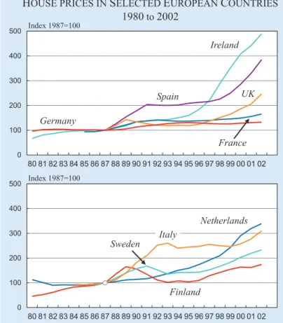
1. IntroductionHouse prices have risen rapidly in most EU member states and in many other countries in recent years, though not uniformly. Between 1992 and 2002 prices in Ireland rose by 250 percent in nominal terms but in western Germany by only 10 percent (ECB 2003 b, Deutsche Bundesbank 2003).
Figure 5.1 illustrates the experience of the EU states. Spanish house prices have risen steadily since that country’s accession. House prices in Britain did not recover their 1989 levels until 1997 but have risen rapidly since then. French prices have been stable with some recent rises.
Other states also show a variety of patterns. Finland and Sweden experienced substantial price falls in the early 1990s. House prices in the Netherlands rose very rapidly through the 1990s, but this was the first coun-try in which prices stalled after the recent boom. Italy shows substantial increases but a volatile pattern. As we emphasise below, however, the quality of the data varies considerably across Europe and not too much significance should be attached to these differences. Since 2000, however, there have been significant rises in all states except Germany and the Netherlands. There is extensive discussion in the press of a house price bubble and of the possibility of a house price crash. However most such discussion simply reflects a belief that what goes up may come down. More sophisticated commentators note that multiples of house prices to incomes are at historically high levels in many places (for example IMF 2004). But this is an indicator that house prices are too high only if there is a “natur-al” ratio of house prices to incomes, to which prices will nec-essarily revert. The ratio of typi-cal mortgage interest payment to income – a more immediate mea-sure of affordability for most households – is low as a result of falls in nominal interest rates. A view on the “appropriate” level of house prices requires more exten-sive analysis of both the demand for housing services and the nature of residential housing as an asset category.
In the UK, house price inflation has become a central issue for monetary policy. Within the eurozone, the issues are different. Despite the adoption of a com-mon com-monetary policy, the hous-ing markets of different member states have behaved in divergent ways. In Britain, Spain and Ireland – which have seen the most rapid escalation of house prices – mortgage finance is gen-Figure 5.1
erally linked to short-term interest rates. In most other eurozone countries, home loans are based on long-term interest rates (although with considerable variation in the terms of early repayment). As a result, the housing markets of these countries may be less sensitive to interest rate fluctuations.
These links between monetary policy and the housing market mean that what happens to housing has a macroeconomic significance greater than can be attached to events in other product markets. This gives wider significance to some fundamental ques-tions about European housing. How far away is Europe from a single housing market, in which the determinants of house prices are similar in Helsinki and Lisbon? Is there likely to be convergence between price levels in different states, and at what rate? And what are the implications of these housing market issues for the wider process of economic integration?
It is difficult to give even provisional, far less defini-tive, answers to these questions. Our purpose instead is to begin a description of the analytical framework which is needed to investigate such questions and the data which would need to be assembled to resolve them. Given the importance of the housing market to
the European economy, it is remarkable how little is under-stood about its characteristics. Few of the questions which are extensively analysed in securities markets have even been posed for the housing market, and data on house prices is not collected across Europe on a comparable basis. A great deal of knowledge and information exists, both among private businesses and in government agencies, but it is not assembled in any systematic fash-ion. This is an appropriate task for the European Central Bank. In 2003 it published a prelimi-nary study of house prices across the fifteen then members of the European Union. However the quality of this information is very uneven. There are many unre-solved issues even in the interpre-tation of the data.1Nor do these surveys allow meaningful com-parisons of levels (as against trends) of house prices between countries. It is therefore not possible to begin an assessment of the extent of convergence and diver-gence within the eurozone.
2. The price of accommodation
The economic analysis of house prices, like all prices, begins from supply and demand. Housing is both a product and an asset class, and much of the complexity of housing economics follows from this duality.
House prices are an element of the total price of accommodation, and Table 5.1 illustrates the vari-Box 5.1
What is a bubble?
“If the reason the price is high today isonlybecause investors believe that the selling price will be high tomorrow – when ‘fundamental’ factors do not seem to justify such a price – then a bubble exists” (Stiglitz 1990).
We broadly follow this definition, which helps to distinguish a bubble from a period of overvaluation. A bubble has, as a necessary condition, a predominance of “noise traders” – people whose trading behaviour is based on considerations other than fundamental value. Examples of such behaviour are momentum trading (chasing upward trends) or “technical analysis” (decisions based on patterns supposedly detected from charts). Noise trading may also result from simple ignorance or disregard of principles of asset valuation. This latter factor is obviously important in housing markets, where most buyers and sellers are inexperienced.
Because there is considerable uncertainty about fundamental values, there can be wide disagreement and substantial fluctuations, which will with hindsight include episodes of substantial overvaluation, even in the absence of noise trading. A prevalence of noise trading is necessary, though not sufficient, for the emergence of bubbles, in which prices lie outside the range of reasonable estimates of fundamental value. Noise traders incur substantial risk of loss, but trading during bubbles is also risky for investors who are not themselves noise traders, and are aware of fundamental values, because once prices lose any anchor on fundamental values there are no bounds to the range of their possible fluctuation. In Keynes’ words, markets can be wrong for longer than investors can stay solvent.
The distinction is complicated by the observation that even in extreme bubbles purported rationalisations in terms of fundamental values are offered for extravagant prices. As the investigations of New York State Attorney General Eliot Spitzer showed of the dot-com boom, however, these rationalisations were often not believed even by the authors themselves.
1There are three broad classes of method of measuring house price
movements:
– average transactions prices, adjusted to reflect the mix of the hous-ing stock
– repeat sales indices, based on sequential observations of sales of the same property
– hedonic indices, which rely on regression analysis of the relation-ship between prices and the characteristics of the housing stock. Each measure is in principle different and in practice can give sub-stantially different results. US data (see McCarthy and Peach, 2004) show the repeat sales index increasing substantially faster than a hedonic index, while in the UK in 2003 hedonic indices recorded annual house price inflation at times 10 percent higher than mea-sures based on average transaction prices. Thus even if the quality of the base data is high (which is true for the UK and the US but not for most European countries) the measurement of prices is subject to considerable uncertainty.
ous components of the cost of accommodation. These costs are partly a function of the monetary value of the house and partly a function of the size of the house. The table calculates the total cost of accommodation using three different figures for the price of housing services. The total cost of accom-modation, as a proportion of all household expen-ditures, falls in a range 19 percent to 36 percent. This is the key figure in considering the “affordabil-ity” of housing.
The price of housing services is determined by the supply of and demand for accommodation. As in all markets, a fall in the price of accommodation leads to an increase in demand for housing. What is meant by increased demand for housing is complex, howev-er, because houses are commodities with many dimensions. The increase in demand for housing that results from a fall in the price of accommodation or housing sservices does not necessarily, or commonly, take the form of a demand for more houses. (Although it may do so as a result either of increased demand for second homes or the formation of new smaller households.).
Households may instead respond to a fall in the price of housing by looking for more space, or a better location, or a combination of the two. While addi-tional houses may be in elastic supply, the capacity of the construction industry to meet the demand for more space in better locations is limited even in the
long run. Rising house prices do not therefore necessarily stimu-late a boom in new construction. This multi-dimensional nature of housing as commodity leads to the wide diversity in the characteristics of housing markets. In the central areas of the United States, popula-tion is sparse, and larger towns are not necessarily organised on the radial patterns common to European towns and cities. Shopping and commercial facili-ties are dispersed rather than focused on a central area. Locational premia for proximity to the centre are small and may, for derelict downtown areas, be nega-tive. Desirable residential areas are generally simply those in which other rich people choose to live.
In areas such as these housing is in essentially per-fectly elastic supply. Prices are low and stable, mov-ing in line with incomes (or buildmov-ing costs, which fol-low a similar time series). In Iowa, for example, the ratio of average house price to personal income per capita varied only between 1.7 and 1.9 over the peri-od 1985–2002 and the highest ratio was reached in 2002. In neighbouring Nebraska, the ratio was in the range 1.8 to 2.1 over the same time period and the peak of 2.1 was observed in 1985 (Case and Schiller 2003).
In coastal states of the US, and in Europe, typical ratios of house prices to incomes are much higher and more volatile. In Iowa or Nebraska, people are simply buying shelter; in California or Munich, the locational characteristics of a house have a major effect on demand and hence on the price of housing services. And in congested areas there are other reasons why a house is more than a structure and a plot of land: it can only function as a home with a supporting infrastruc-ture – road access, utility connections, street cleaning and waste collections, schools and medical facilities. The provision of such infrastructure is costly and its availability limited. Some of these infrastructure costs are paid by the housebuilder or first occupier; others fall on public authorities. But the value of the house will reflect their quality and availability. In addition, planning rules may restrict building even on land that is in plentiful supply, creating “value” through the process of planning approval.
Table 5.1
The price of accommodation in euros (UK, Spain 2002)
(1€= 0.675 GBP)
UK Spain Maintenance and repairs 891 519 Utilities 1319 1043 Furnishings 1244 1005 Property taxes 1191 385
4645 2952
Cost of housing services – at 1% of capital
value of average house price 1852 1423 at 2% of capital value 3704 2846 at 5% of capital value 9259 7115
Total non housing household expenditure 25185 18745
Accommodation costs as % of all expenditure
– at 1% 21% 19%
– at 2% 25% 24%
– at 5% 36% 35%
Source:Office for National Statistics, UK (2002), Instituto Nacional de Estadística,
http://www.catastro.minhac.es/estadistica/interactivo2/default.htm, Ministerio de Fomento (2002).
2.1 Locational characteristics
Attractive locational characteristics fall into three main groups:
(i) Proximity to central commercial areas. Houses in large cities command substantial premia and in general the closer they are to the centre the larger are these premia.
(ii) Scenery and climate. Certain areas are particular-ly pleasant places to live.
(iii) Glamour. Certain areas are particularly fashion-able – a “good address”. Such fashions may be transitory but usually are not: a good address will attract amenities which ensure that it retains that aura. University towns often have these charac-teristics.
The recent US house price boom has been concen-trated in a small number of states: essentially, the Northeast, California, and Hawaii (HSBC 2004a, Case and Schiller 2003). These were already the states with the highest ratio of house prices to per capita income and they have experienced much greater volatility of house prices than Midwestern states such as Iowa and Nebraska. All these coastal or island states enjoy at least one of the benefits of (i), (ii), and (iii) above and, in the case of California, all three. After Hawaii, California has the highest ratio of prices to per capita income of any state of the Union (ca. 9:1 in 2004).
There is wide – although not complete – agreement among prospective buyers on what constitutes good and bad locations. If the ranking of locational quali-ty is objectively defined, and houses have already been built in all the best available locations, Figure 5.2
illus-trates how the price of housing services is determined. OB represents the price of housing services in the best location. At D, the poorest location at which it is worth building, the cost of housing services is entire-ly determined by construction costs, as in Iowa and Nebraska.
The overall value of the housing stock is then OABCD. The level of house prices is determined by the level of building costs, OA, and the slope of the location gradient, BC. For the UK, the average level of house prices in 2004 is €225,000 (equal to about nine times per capita income, as in California) and the building cost of an average house (90 sq m) around €100,000 (although the provision of associated ser-vices may add up to 40 percent to the construction cost of a dwelling).
The area ABC then represents about 55 percent of the value of the UK housing stock and can, as a first approximation, be described as the value of UK house building land: the area OACD, representing about 45 percent of the value of the UK housing stock can, as a first approximation, be described as the value of the structures.
The steepness of the gradient, BC, is determined part-ly by the degree to which houses are differentiated by locational quality – little in Nebraska, extensive in London – and partly by the inequality of income. Houses are what Fred Hirsch (1976) called a position-al good. The richest people will position-always live in the best houses, but the aspirations of poorer people will drive up the price they have to pay. At the same time, com-petition among the rich to secure the very best houses will drive up their prices to reflect their ability to afford them.
An increase in demand for hous-ing services might come either from a demand for additional housing space overall (as from demographic factors) or from a demand for the locational char-acteristics that housing services offer (people living in less favoured locations using their growing incomes to buy a more convenient house). Demand for structures can be satisfied by additional house-building; demand for positional compo-nents cannot be, and simply leads to an increase in the price of these positional characteristics. Figure 5.2
The key feature of the positional good is that even if the good can itself be replicated, the positional char-acteristic cannot be. If Eaton Square is the “best address”, and the number of houses in Eaton Square doubles, then the title of “best address” attaches to a subset of houses in Eaton Square (or transfers to an altogether different location.)
This effect can partly be mitigated by substituting space for the positional characteristics of houses – households settle for a larger house in a less favourable location – but this process leads to a steady fall in the price of space relative to other characteris-tics of houses. This is why it is easy in most European countries to buy large but poorly located houses for low prices per square meter of accommodation.
European economies are more like California and New York than Iowa and Nebraska. Average houses in Europe fetch, on average, around ten times average national per capita income. In the UK the average house price is currently around €225,000, nine times per capita income of €25,000; in Germany a represen-tative row house costs €260,000, twelve times per capi-ta income of €22,000.
2.2 Locational gradients
Among the larger EU members, two countries, France and the UK, have a dominant city that is both the political and commercial capital: Greater Paris and Greater London are among the largest cities in Europe, accounting for about one quarter of the pop-ulation of these countries. In both states the gradient of house prices slopes steeply towards the centre of these cities and the most favoured areas within them (Kensington/Belgravia, Paris VIII and XVI) have the highest prices in Europe. In both countries there are secondary, but much lower, peaks in secondary cities such as Birmingham, and Lyon has a scenery and cli-mate gradient towards the PACA (Provence – Alpes – Côte d’Azur) region.
Germany, in contrast, has had no similarly dominant city, and like Spain and Italy has different political and commercial capitals. The most expensive German city is Munich, which is a business centre, houses the state government of Bavaria and benefits from favourable scenery and climate. Munich house prices are around 50 percent more than the all-German aver-age (Deutsche Bundesbank 2003, Bulwien AG 2003), which suggests that locational dispersion may be less marked in western Germany than in France or Britain
(it seems inappropriate to include the East in these comparisons).
Most of the population of the Netherlands is located within the North Sea coastal strip, and the country can be described as a linear city with numerous com-mercial centres. The locational gradient found in the Netherlands is correspondingly small: surveys suggest (VROM, 2000–4) that at the peak of the Dutch house price boom differentials between the various provinces of Holland had virtually disappeared, although the subsequent weakness of prices has affected less favoured (less central) parts of the Netherlands more than the congested areas of Nord and Zuid Holland. In Britain, by contrast, house prices in the most expensive region (London) average two and a half times those in the cheapest (Scotland) (Halifax, 2004).
3. Underlying influences on the supply and demand for housing services
Houses take time to build, and the entire capacity of a national construction industry cannot increase its physical housing stock by more than, say, five percent a year, and usually by much less. Thus, while the long run elasticity of supply of shelter (structures) is very high, the short run elasticity is low, although this elas-ticity may be higher in smaller areas.
Within the overall parameters of population and housing stock, translation of these figures into supply and demand for housing depends on a number of fac-tors. Some of these are cultural influences indepen-dent of the housing market itself, but the price of housing may in turn have some effect on these cultur-al influences, such as the rate of household formation.
(a) Conversion of overall population into numbers of households. This depends principally on the age structure of the population: children tend to live in households with adults, older people tend to live in smaller households (as children leave home and partners die). Cultural factors are relevant, particularly the age at which children establish their own households, the degree to which elderly people live with children, and the rate of house-hold dissolution through divorce and relationship breakdown. These cultural factors are, in turn, influenced by economic factors such as house prices and overall income levels.
(b) The rate of depreciation and obsolescence of the existing housing stock. Depreciation of the hous-ing stock is of two kinds: physical depreciation, the physical deterioration of housing through time, weather and wear and tear; and economic depreciation, any particular configuration of the housing stock becomes less appropriate, over time, for current needs. Economic depreciation is, in turn, a function of a range of factors
– other economic change (for example, shifts in the location of industry, changes in the avail-ability of communications or transport) – changes in prices of other goods (for example,
energy, domestic servants, washing machines) which change the relative attractiveness of dif-ferent houses or the cost of housing relative to other goods
– rising incomes (which raise expectations of, for example, kitchen facilities, ambient temperature) – changes in preferences (for example, demand for rural versus urban locations, the identity of glamour locations).
Thus, the rate of economic depreciation will depend on the overall rate of economic growth and on trends in the prices of goods complementary to housing. The rate of economic depreciation will also depend on the average age of the housing stock, which varies substantially across Europe. Finland and Greece have the youngest housing stock in Europe (probably as a result of recent migration to urban areas), fol-lowed by the Netherlands, whose stock suffered extensive wartime damage. The UK has the oldest housing stock. Eastern Germany and the ex-commu-nist accession states have inherited a housing stock prone to particularly rapid depreciation in both physical and economic terms.
(c) Demand for second homes. This depends on income inequality and cultural preferences. Many Scandinavian households have small sum-mer cottages. Country residences are fashionable among affluent Londoners and Parisians (but only affordable by the rich). Few Dutch or German households have second homes in the same country.
(d) The efficiency of utilisation of the housing stock. In all countries, houses are empty because of – economic obsolescence (see above)
– inefficiencies in the housing market: difficul-ties in organising simultaneous sale and pur-chases for owner occupiers, voids in the rental sector, especially in the social housing sector.
4. The relationship between house prices and the price of housing services
If a home provides a stream of services fixed in value relative to the general price index and not subject to depreciation, then the value of that house is the value of that stream of housing services capitalised at the long term real interest rate. Thus the long term real interest is a key influence on the appropriate level of house prices.
The recent rise in house prices should therefore be seen in the context of a substantial rise in the price of other assets, including the most directly comparable asset class: long-dated indexed bonds. In the UK, the earliest and largest issuer of these securities, real yields have fallen from around four percent in the mid-1990s to below two percent today. The UK mar-ket has been influenced by some technical factors con-nected with the funding of pension schemes, but there have also been substantial rises in the prices of long-dated indexed securities in other countries, including the US – where Treasury Inflation-Protected Securi-ties (TIPS) were first issued in 1997 – and in the prin-cipal eurozone issuer, France.2The first French long-dated bond was issued in September 1998 to return 3.4 percent, and the yield on these securities has since fallen to 2.4 percent. This factor alone is sufficient to explain most of the rise in French house prices over the period.
Indexed bonds are appropriately classed as riskless assets because these securities allow complete hedging of a desired consumption stream. However the price of these securities has proved volatile in practice,3and this volatility translates into uncertainty about the appropriate level of house prices. The yields obtain-able on indexed bonds during the late 1990s seem high relative not only to current yields but to conventional expectations of long-term interest rates, including his-toric bond yields in periods of low inflation. This may be attributable to unrealistic expectations of future equity returns during the stock market bubble associ-ated with the “new economy”.
The future prospects for long-term interest rates depend in large measure on the range of investment opportunities and supply of savings in the world
2The first French issues were linked to the French price level. Some
more recent issues are tied to European inflation.
3If there were undated indexed bonds, their price would have been
more volatile still. The real present value of the repayment on a con-ventional 30 year bond is low because it is fixed in nominal terms, but that of a 30 year indexed bond, which is fixed in real terms, is substantially higher.
economy. The most important influences on these in the short term are the large US budget deficit, aggra-vated by the deterioration in the fiscal position of European economies associated with the failure to observe the Stability and Growth Pact, the substantial savings being generated in East Asia and the invest-ment opportunities generated by rapid economic growth in India and China. On the other hand, any resolution of the problem of US fiscal and trade imbalances would be likely to lead to an increase in savings and to greater demand for risk-free assets.
The housing market, however, is dominated by unso-phisticated investors whose views on interest rates may be little influenced by fundamental factors in the world economy. Although it is these fundamental fac-tors that underpin the long-term trend of house prices, short-term movements will be more affected by household expectations of interest rates, which will in turn be influenced by the rates at which mortgages are advertised. It is striking that the three European coun-tries with the largest recent increases in house prices – Ireland, Spain and the United Kingdom – are coun-tries in which mortgage finance is principally related to short-term interest rates. In the two eurozone mem-bers, these rates continue to be very low. In the UK, the state of the housing market has been a major influence on decisions by the Bank of England to raise interest rates. The relationship between fixed and variable rate mortgage finance and the housing mar-ket is a major issue in the conduct of European mon-etary policy (Miles 2004).
5. The characteristics of houses versus bonds
Houses do, however, differ significantly from indexed bonds in their characteristic as assets. The most important of these differences are risk, tax, physical depreciation (through wear and tear for a house, through impending maturity for a bond), economic growth, economic depreciation or appreciation, trans-actions and agency costs. We consider each of these elements in turn. We do so for three types of houses – one owned outright, one owned with a 75 percent mortgage, and one owned for letting. We compare these asset characteristics with those not only of indexed bonds but also relative to commercial proper-ty – retail, office and industrial and equities. For con-creteness, we suggest specific values for the differences in yield which might follow from the differences between the characteristics of the asset classes. These
numbers are essentially illustrative, and alternative values can readily be substituted in Table 5.2.
5.1 Risk
Within the capital asset pricing model, equities are normally treated as the dominant asset class – risk is measured relative to a market equity portfolio. A cur-rent consensus puts the equity risk premium in the range 300–500 basis points (see, for example, Dimson, Marsh and Staunton 2002) All property asset classes are correlated with equity prices, but not perfectly, and property price movements show lower amplitude than equity prices. We set the risk premium at four percent for equities and two percent for rented property.
The position of owner occupiers is more complex. It is difficult to construct a well diversified portfolio if, as is true for most owner occupiers, one single element accounts for more than 100 percent of net assets. But this is not necessarily the correct perspective since a house acts as a hedge against future housing costs. This hedge may be very attractive, since the house is the one the occupier has selected to live in. We assume no risk premium for a house owned outright.
A purchaser with a mortgage is exposed to greater risk. Interest and repayment of capital are defined in nominal terms, but the income stream from which repayments are made will move broadly in line with inflation, as will the value of the asset – the house – against which the loan is secured. Higher than expect-ed inflation helps wipe out the value of the debt, while falling inflation – as in the 1990s – can mean that bor-rowing to finance home ownership may be more bur-densome than anticipated. If interest rates are vari-able the home buyer is exposed to uncertainty about the nominal value of repayments; if interest rates are fixed, the home buyer is exposed to uncertainty about their real value. However, the lack of interest in infla-tion-linked mortgages suggests that this risk is not perceived as very large. We set the premium associat-ed with this inflation-relatassociat-ed risk, rather arbitrarily, at one percent.
5.2 Tax
The tax position varies across EU member states. However investors in property and equities are nor-mally subject to a tax on income and capital gains from these assets. The tax is generally levied on nom-inal income, although there may be some relief for
capital gains. We have put tax at 100–200 basis points for all these assets.
Some countries impose tax on the imputed income from owner occupation, but many do not and where tax is charged its basis is rarely onerous. Tax relief is frequently denied or limited on interest paid on mort-gage borrowing. Capital gains tax is not generally paid by owner occupiers. We have set the tax at zero for property owned outright and one percent for owner occupiers with a 75 percent mortgage. The most usual tax treatment of indexed bonds is that the coupon is taxed but not the indexation of principal. Tax here is estimated at 1/2 percent.
5.3 Economic growth
As a first approximation, rents and profits may be expected to rise in line with overall economic growth. It is not obvious whether output or per capita output is more relevant. This figure has been set at 2 percent.
5.4 Physical and economic depreciation
Physical depreciation is the expenditure required to maintain the physical characteristics of an asset. Economic depreciation is the decline (or appreciation) of the value of an existing asset with unchanged phys-ical characteristics relative to newly produced versions of that asset class.
Equities suffer no physical depreciation, but do expe-rience economic depreciation because established companies must continually give way to new ones, and therefore (unless the overall profit share increas-es) the profits of a fixed population of companies will decline relative to national income. This economic depreciation is set at one percent. Although actual indexed bonds depreciate (because having been issued at higher historic levels of real interest rates they gen-erally stand at premia to their issue price in real terms), the comparison made here is with hypotheti-cal perpetual bonds.
For office and industrial properties, physical and eco-nomic depreciation should be viewed together. These structures are generally replaced before the end of their physical lives because they can no longer be eco-nomically adapted to changing business needs. The combined effect is set here at five percent. Shops depreciate less than other commercial properties because much of their value lies in site rather than structure.
Physical depreciation of houses relates to structures but not land. In addition, houses are likely to experi-ence economic appreciation because of increased pressure on a relatively fixed supply of non-shelter characteristics as incomes rise. Moreover, while mod-ern industrial and office buildings are in almost all cases preferred to older industrial and office proper-ties, traditional characteristics of houses are often positively valued. Taking all these factors together, physical depreciation of two percent and economic depreciation of zero is assumed for housing.
5.5 Transaction costs
These comprise taxes on property and share transac-tions, legal costs, agency and brokerage fees, and bid–offer spreads. Such charges vary considerably across European countries. Amortised over a period of years, these costs are set at one percent for all property. Transactions costs are much lower for equities but turnover much higher, and one percent is used here also. Transactions costs for indexed bonds are negligible.
5.6 Agency costs
Agency costs are associated with property manage-ment and more broadly with the information asymme-tries and moral hazards of the type that owner occu-pation avoids but are inescapable whenever ownership and control of assets are in the hands of distinct par-ties. Agency costs are set at one percent for all assets except owner-occupied houses and indexed bonds.
For owner occupied property, the “required yield” of Table 5.2 equates to the price of housing services required in the measurement of the cost of accommo-dation in Table 5.1. This figure equates to about 10 percent of total household expenditure. There is no “natural” figure for this ratio. But such a figure is not unmanageable in relation to overall household bud-gets. None of the other “required yields” in Table 5.2 are obviously anomalous. These required yields are towards the upper end of the range of yields current-ly available for these asset classes in European mar-kets, suggesting, plausibly, that most assets are cur-rently somewhat expensive.
An analysis of this sort cannot hope to give a “cor-rect” value for house prices. But some provisional conclusions can be drawn.
a) The price of housing services is sensitive to quite small changes in the assumptions of Table 5.2 and
to changes in the economic environment. The range of house prices that could be justified by ref-erence to fundamental values is therefore quite wide. House prices may therefore be expected to be volatile around their long-term trend, and there is sufficient uncertainty about that trend for it to be difficult to identify clearly either over or under val-uation.
b) The fundamental value of house prices in the long run is particularly sensitive to the level of long term real interest rates. It should therefore not be surprising that the substantial reduction in real interest rates from 1997 has been followed by sig-nificant house price increases. There is no discus-sion of a “bubble” in indexed bonds: indeed the yields which were available on such bonds until the late 1990s seem very high relative to historic expe-rience, reflecting unrealistic expectations of returns from equities as a result of the very real “bubble” in stock markets. Current real yields are more con-sistent with bond yields experienced in non infla-tionary times.
c) Following from this, the strength of house prices is not surprising given the extent of gains in almost all other asset markets. Even in the UK, which has (apart from Ireland) experienced the most rapid increases, it was only in 2004 – after four years in which the trend of equity markets was down and that of houses strongly upwards – that house price increases matched share price increases after the cyclical lows established in 1982.
d) There is no evidence of a ‘bubble’ in the housing market comparable to the ‘bubble’ in technology stocks in 1999-2000, or that in Japanese equities in 1985–89. In both these episodes, prices became divorced from any realistic calculation of the
potential earnings capacity of the underlying asset and purchasers were principally motivated by the expectation that the paper they purchased could rapidly be sold at a higher price to someone else. House prices may currently be expensive but are not fantastic, and most purchasers of houses make these purchases with the intention of enjoying the services of the properties they buy.
6. Tenure choice
There are large variations across Europe in tenure choice. In Britain and Spain, over 70 percent of hous-es are owner-occupied, but this figure is below half in Germany and Switzerland. The countries with high rates of owner occupation have experience of both rapid and volatile inflation. High inflation tends to increase the tax benefits of owner occupation because the nominal yield on assets is taxable, and so the effec-tive tax rate on real returns increases. The tax advan-tage has this character because “imputed income” from housing is tax free or lightly taxed; the tax bur-den is lower if the owner and occupier are the same person and is greater at higher inflation rates. This tax advantage is increased if nominal mortgage interest payments are wholly or partly tax deductible, and if capital gains by owner occupiers are tax free. Volatile inflation increases the hedging benefits from owner occupation (although it also increases the risks to which mortgage borrowers who match a nominal repayment stream with a real income stream are exposed).
However, as is evident from Table 5.2, owner occu-pation is generally economically more attractive than
Table 5.2
Required adjustments to returns for housing and other assets relative to indexed bonds (basis points)
Housing, owned outright House, 75% mortgage Housing, tenanted
Shops Offices Ind.
Property
Equities
Risk 0 100 200 200 200 200 400
Tax 0 100 150 150 150 150 150
Growth -200 -200 -200 -200 -200 -200 -200
Physical and economic depreciation
200 200 200 300 500 500 100
Transactions costs 100 100 100 100 100 100 100
Agency costs 0 0 100 100 100 100 100
Total 100 751) 550 650 850 850 650
Post tax real yield on indexed bonds
150 150 150 150 150 150 150
Required yield 250 225 700 800 1000 1000 800
Note:1)25% of 300
tenancy, offering tax advantages and eliminating agency costs. Against this, transactions costs are lower in the rental sector for people who move fre-quently, and gaps in the credit market may make owner occupation difficult for some households. There will always be some low-income households that are unattractive to any lender. Often, these householders will not be sought after as tenants either. This market segment is handled everywhere through social housing.
Because mortgage lending is offered on much more attractive terms than other consumer lending, household cash flow profiles are substantially influ-enced by the practices of mortgage lenders. This was particularly important during the period of rapid inflation (and associated high nominal interest rates), when initial mortgage repayments were high but fell rapidly in real terms because repayments were nominally fixed in nominal values for the term of the mortgage. Today, initial repayments are lower (relative to the size of the mortgage) but decline much more slowly over the life of the mortgage. Thus nominal interest declines are likely to have had an influence on prices as well as drops in real inter-est rates.
A further complication arises through the calculation of depreciation in the owner occupier segment. While a house may have an indefinite life, its owner occu-piers do not: in this sense an owner-occupied house may be perceived as a depreciating asset.
There are two extreme assumptions:
– Households behave as if they live forever, if not lit-erally then in the shoes of their children/grand-children
– Households regard their house as worthless on the death of the last partner.
In the latter case, such households should aim to die with zero net assets. It does not appear that many households do this, which suggests that the first assumption may be closer to the truth, although it may also reflect the limitations of institutional arrangements allowing old people to realise the cap-ital locked into their houses. People can sell their houses and rent equivalent property with the pro-ceeds of a purchased annuity, but this is not particu-larly attractive either logistically or financially. There are schemes of equity release that allow people to borrow against the security of their house with repayment at death. Other schemes involve sale with life tenancy.
7. The future of house prices
The behaviour of technology stocks in the period 1997–2000 represented one of the largest speculative bubbles in history, ranking along with Japanese stocks and real estate in the 1980s, Florida land speculation in the 1920s, railways and railroad booms in the nine-teenth century, and Dutch tulip mania. It is this recent experience that causes talk of a housing “bubble”. There is no such bubble in the European housing mar-ket. There may be an element of overvaluation, al-though that is not clear either.
This does not mean that expectations do not have an influence on house prices. They do, and from the analysis of Table 5.2, they should. There is clear evidence from the United States that expectations have been unreasonable, and this has an upward impact on current prices which will some day be removed.
In common with other markets that have speculative influences, house prices exhibit a pattern of positive serial correlation in the short run and mean reversion in the long run. Specifically, this means that if prices rose last month, then they are more than averagely likely to rise next month – but that if sufficiently long-time scales are examined, periods in which prices rise by more than the long-term trend are followed by periods in which prices rise by less than the long-term trend.
The reason this information is even less useful than it sounds is that while such patterns can be identi-fied with hindsight, the interval at which the short run becomes the long run is not fixed. Therefore while it is possible to assert with considerable confi-dence that the current period of rapid house price inflation will be followed by a period of slow or even negative house price rises, there is no good way of predicting whether that period will start tomor-row or in three years’ time. And from the perspec-tive of someone who is thinking of buying a house today – and seeks an answer to the question – that difference is crucial.
The available data does not allow us to make con-fident statements about the relative levels of prices in different European countries. This is an impor-tant question, and European agencies should undertake the data collection which would make it possible. There is some evidence of convergence during the house price boom. For example, the gap
between apparently high prices in Germany and significantly lower prices in the Netherlands has narrowed, and Ireland and Spain, with particularly rapid rises, seem to have started from a low base. But this reflects processes of internal adjustment within the countries themselves rather than the convergence at the level of Europe, or the eurozone, as a whole.
8. Conclusions
1. The level of house prices in Europe today is not manifestly out of line with fundamental values. House prices at current levels do not impose demands on household budgets which are unsustainable, nor do they seem substantially inconsistent with valua-tions currently applied to other assets.
2. The range of uncertainty about the “correct” level of house prices is very wide. House prices will contin-ue to be volatile and it is possible, but not at all cer-tain, that from a long term perspective current values will appear high.
3. The present period of rapidly rising house prices will be followed by a period in which house prices rise very slowly and may even fall. Such a period might be about to start, it may have already started, or it may not.
4. People who make confident projections of future house price trends (“house price inflation will slow later this year”, ‘”house prices are 20 percent overval-ued”) have no scientific basis for the knowledge they claim. But they may be right anyway.
References
Bulwien AG (2004), Property Market Index 1975 to 2003, Residential
and Commercial/Rents and Prices, Munich.
Case, K. E. and R. J. Schiller (2003), “Is There a Bubble in the Housing Market? An Analysis”, Brooking Papers on Economic
Activi-ty, no. 2.
Deutsche Bundesbank (2003), Monthly Report Price indicators for the
housing market, September.
Dimson, E., P. Marsh, and M. Staunton (2002), Triumph of the
Optimists: 101 Years of Global Investment Returns, Princeton
University Press, Princeton.
European Central Bank (2003b), Structural Factors in the EU
Housing Markets, Frankfurt am Main.
Federal Statistical Office of Germany (2002), Laufende
Wirtschafts-rechnungen.
Halifax plc (2004), Regional House Price Indices.
Hirsch, F. (1976), The Social Limits to Growth, Harvard University Press, Cambridge, MA.
HSBC Bank plc (2004), “The US Housing Bubble – The Case for a Home-Brewed Hangover”, London, June
IMF World Economic and Financial Surveys (2004), World Economic
Outlook,Washington D.C, April.
Instituto Nacional de Estadística (2002), Encuesta Continua de
Presupuestos Familiares (base 1997, dat a 2002).
McCarthy, J. and R. W. Peach (2004), “Are Home Prices the Next “Bubble”?”, Economic Policy Review, 10 (3).
Miles, D. (2004), The Miles Report on the UK Mortgage Market, London, HMSO.
Ministerio de Fomento (2002), Índices de precios de las viviendas;
estadísticas del precio medio del m2.
Netherlands Ministry of Housing, Spatial Planning and the Environment (VROM, 2004), Cijfers over Wonen.
Office for National Statistics (2002), Family Expenditure Survey.
Stiglitz, J. (Spring 1990), “Symposium on Bubbles,” Journal of